A Review of Geochemical Modeling for the Performance Assessment of Radioactive Waste Disposal in a Subsurface System

Abstract

Radionuclides are inorganic substances, and the solubility of inorganic substances is a major factor affecting the disposal of radioactive waste and the release of concentrations of radionuclides. The degree of solubility determines whether a nuclide source migrates to the far field of a radioactive waste disposal site. Therefore, the most effective method for retarding radionuclide migration is to reduce the radionuclide solubility in the aqueous geochemical environment of subsurface systems. In order to assess the performance of disposal facilities, thermodynamic data regarding nuclides in water–rock systems and minerals in geochemical environments are required; the results obtained from the analysis of these data can provide a strong scientific basis for maintaining safety performance to support nuclear waste management. The pH, Eh and time ranges in the environments of disposal sites cannot be controlled, in contrast to those under experimental conditions in laboratories. Using a hypothetical error mechanism for the safety assessment of disposal sites may engender incorrect assessment results. Studies have focused on radionuclide reactions in waste disposal, and have offered evidence suggesting that these reactions are mainly affected by the geochemical environment. However, studies have not examined the thermodynamics of chemical reactions or interactions between water and minerals, such as the surface complexation and adsorption of various nuclide-ion species. Simple coefficient models have usually been applied in order to obtain empirical formulas for deriving Kd to describe nuclide distributions in the solid or liquid phase in water–rock geochemical systems. Accordingly, this study reviewed previous research on the applications of geochemical models, including studies on the development of geochemical models, sources of thermodynamic databases (TDBs) and their applications in programs, the determination of the adequacy of TDBs in surface complexation models and case studies, and the selection and application of activity coefficient equations in geochemical models. In addition, the study conducted case studies and comparisons of the activity coefficients derived by different geochemical models. Three activity coefficient equations, namely the Davies, modified Debye–Hückel, and Pitzer equations, and four geochemical models, namely PHREEQC, MINEQL+, MINTEQA2, and EQ3/6, were used in the study. The results demonstrated that when the solution’s ionic strength was <0.5 m, the differences in the activity coefficients between the Davies and modified Debye–Hückel equations were <5%. The difference between the Pitzer and Davies equations, or between the Pitzer and modified Debye–Hückel equations in terms of the calculated activity coefficients was <8%. The effect of temperature on the activity coefficient slightly influenced the modeling outputs of the Davies and modified Debye–Hückel equations. In the future, the probability distribution and uncertainty of parameters of Kd and the equilibrium constant can be used in geochemical and reactive transport models to simulate the long-term safety of nuclear waste disposal sites. The findings of this study can provide a strong scientific basis for conducting safety assessments of nuclear waste disposal repositories and developing environmental management or remediation schemes to control sites marred by near-surface contamination.

1. Introduction

A nuclear regulatory authority must provide a permit for the construction and operation of a repository for radioactive waste disposal. Therefore, a comprehensive multidisciplinary approach to safety assessment is required in order to determine whether the repository can safely dispose of radioactive nuclear waste. Currently, radioactive waste disposal often employs a multibarrier system composed of engineering barriers and natural barriers. The engineering barrier system includes the waste form, waste package, and concrete; furthermore, a buffer material is combined with backfill material to act as a physical and chemical barrier to retard the migration of radionuclides. The multibarrier system is designed for the isolation of radioactive waste from the biosphere. The evolution of repositories for geological disposal involves highly complicated coupling processes, including the mechanical stress change (M) of the repositories during excavation and construction, radionuclide decay heat (T) after the repository’s closure, groundwater pressure (H) in the geological environment, and the interactions of various geochemical processes (C) among the groundwater chemical species, rock minerals and possibly released nuclides. The chemical field plays a crucial role after the disposal site’s closure. Chemical changes occur because of near-field geochemical interactions caused by changes in temperature, the flow field and the stress field. Geochemical evolution affects the chemical composition of groundwater, waste form dissolution and nuclide release. These changes are considered nuclide migration problems in the performance safety assessment of repositories.

Therefore, geochemical models are required during the assessment process to predict the concentrations and chemical speciation of radionuclides entering the environment through different events and processes. A geochemical model is used to describe the water–gas–rock interaction in the aquatic system. The activity calculation method in a geo-chemical model is based on the ion-association theory. When the ionic strength of an aqueous solution increases to a value between 0.5 and 1 mol/kgw, the geochemical model can obtain reliable results. However, when the ionic strength exceeds this limit, a geochemical model based on an ion-interaction theory (such as the Pitzer equation) must be invoked for accurate predictions. There are two kinds of numerical methods for thermodynamic equilibrium modeling that can be applied to the calculation of speciation in aqueous systems, namely (1) the Law of Mass Action and (2) the Gibbs Energy Minimization. In general, two methods can be used to calculate the species distribution from a thermodynamic database. The first method consists in solving a set of nonlinear equations generated by the system’s mass balances and equilibrium constants. The second method involves determining the most thermodynamically stable state by minimizing the reaction’s free energy (the lowest energy state). Both methods are based on establishing the mass balance and chemical equilibrium state of the system. The relationship between the equilibrium constants, free energy, and the related chemical reactions and thermodynamic parameters is described below [1].

The following mass-action law defines an equilibrium constant in a thermodynamic database of a geochemical model:

$$\mathrm{aA}+\mathrm{bB}\rightleftharpoons \mathrm{cC}+\mathrm{dD}$$

(1)

$$\mathrm{K}=\frac{{\mathrm{a}}_{\mathrm{C}}^{\mathrm{c}}{\mathrm{a}}_{\mathrm{D}}^{\mathrm{d}}}{{\mathrm{a}}_{\mathrm{A}}^{\mathrm{a}}{\mathrm{a}}_{\mathrm{B}}^{\mathrm{b}}}$$

(2)

where a, b, c and d are the stoichiometric coefficients of the reactants A and B, and the products C and D, respectively, for the reaction (1). The terms a_A, a_B, a_C and a_D are the activities of A, B, C and D, respectively. K denotes the thermodynamic equilibrium constant.

In general, K can be characterized in the following way for these specific types of reactions: the complexation constant (K) for complex formation/dissolution reactions, the stability constant (K) for redox reactions, the solubility-product constant (Ksp) for dissolution/precipitation reactions, and the distribution coefficient (Kd) and selectivity coefficient (Kx) for sorption reactions. Surface complexation theory describes sorption phenomena based on the surface reaction equilibrium. Such phenomena occur on the surface of materials such as iron, aluminum, silica and manganese hydroxides, as well as on those of humic substances. Accordingly, four models have been proposed, namely the constant capacitance model, the diffuse double-layer model, the triple-layer model, and the charge distribution multisite complexation model. Surface complexation models are still being developed for the description of the adsorption/desorption reactions of nuclides. For example, Marmier [2] reported that cesium can be adsorbed on the surface of silica, and that a surface complexation model (SCM) can describe the adsorption of cesium on the surface of silica. Moreover, BarNes et al. [3] indicated that cesium tends to bind to silica particles in cement hydration minerals. Iwaida et al. [4] observed that cesium can be adsorbed on the silicate chain (C–S–H) of cement. In addition to cesium nuclides, Wang and Turner [5,6] reported that the adsorption of radionuclides is a major concern in water–mineral geochemical reactions with regard to the safety assessment of radioactive waste. They have developed a surface complexation model based on diffusion layer theory to assess the cations (such as Am³⁺, Pu⁴⁺, Pu⁵⁺ and Np⁵⁺) and anions (such as I⁻, IO₃⁻, SeO₃²⁻, SeO₄²⁻ and TcO₄⁻) of radionuclides in clay and various minerals by using chemical thermodynamic and equilibrium constant data.

For equilibrium reactions, the equilibrium constant is temperature-dependent, and can be calculated using the Van’t Hoff equation, as follows: [1]

$${\mathrm{K}}_{\mathrm{T}}{=\mathrm{K}}_{\mathrm{Tr}}\exp \left[\frac{{\mathsf{\Delta }\mathrm{H}}_{\mathrm{Tr}}}{\mathrm{R}}\left(\frac{{\mathrm{T}-\mathrm{T}}_{\mathrm{r}}}{{\mathrm{TT}}_{\mathrm{r}}}\right)\right]$$

(3)

where K_T and K_Tr are the equilibrium constants for equilibrium reactions at the temperature of interest, T, and the referenced temperature, T_r (298.15 K), respectively; ΔH_Tr, is the enthalpy of the associated equilibrium reactions; and R is the ideal gas constant (8.315 J mol⁻¹ K⁻¹).

The equilibrium constant is also pressure-dependent, and can be expressed as follows:

$${\mathrm{lnK}}_{\mathrm{P}}{=\mathrm{lnK}}_{{\mathrm{P}}_{\mathrm{rS}}}-\frac{{\mathsf{\Delta }\mathrm{V}}_{{\mathrm{T},\mathrm{P}}_{\mathrm{rS}}}}{\mathrm{T}\cdot \mathrm{R}\cdot \mathsf{\beta }}\ln \frac{{\rho }_{\mathrm{P}}}{{\rho }_{{\mathrm{P}}_{\mathrm{rS}}}}$$

(4)

where K_P and K_PrS are the equilibrium constants for the equilibrium reactions at the pressure of interest, P, and the reference pressure, P_rs (i.e., the saturated vapor pressure), respectively; ΔV_T,PrS is the volume change of the dissociation reaction at the temperature T and reference pressure P_rs; β is the isothermal compressibility coefficient of water at the temperature T and the pressure of interest, P; and ρ_P and ρ_PrS are the densities of water at the pressure of interest, P, and reference pressure, P_rs, respectively. [1]

The equilibrium constant can also be related to the standard molal Gibbs free energy of a reaction at any temperature and pressure by the following equation:

$${\mathrm{lnK}}_{\mathrm{r}}=\frac{{-\mathsf{\Delta }\mathrm{G}}_{\mathrm{r}}^0}{\mathrm{RT}}$$

(5)

$${\mathsf{\Delta }\mathrm{G}}_{\mathrm{r}}^0{=\mathsf{\Delta }\mathrm{G}}_{{\mathrm{r},\mathrm{P}}_{\mathrm{r}}{,\mathrm{T}}_{\mathrm{r}}}^0{-\mathsf{\Delta }\mathrm{S}}_{{\mathrm{r},\mathrm{P}}_{\mathrm{r}}{,\mathrm{T}}_{\mathrm{r}}}^0{(\mathrm{T}-\mathrm{T}}_{\mathrm{r}})+{\displaystyle {\int }_{{\mathrm{T}}_{\mathrm{r}}}^{\mathrm{T}}{\mathsf{\Delta }\mathrm{C}}_{{\mathrm{r},\mathrm{P}}_{\mathrm{r}}}^0\mathrm{dT}-\mathrm{T}}{\displaystyle {\int }_{{\mathrm{T}}_{\mathrm{r}}}^{\mathrm{T}}{\mathsf{\Delta }\mathrm{C}}_{{\mathrm{r},\mathrm{P}}_{\mathrm{r}}}^0\mathrm{dlnT}+{\displaystyle {\int }_{{\mathrm{P}}_{\mathrm{r}}}^{\mathrm{P}}{\mathsf{\Delta }\mathrm{V}}_{\mathrm{r}}^0\mathrm{dP}}}$$

(6)

where T_r and P_r stand for the reference temperature and pressure, and $\mathsf{\Delta }{\mathrm{G}}_{\mathrm{r},\mathrm{Pr},\mathrm{Tr}}^0$, $\mathsf{\Delta }{\mathrm{S}}_{\mathrm{r},\mathrm{Pr},\mathrm{Tr}}^0$, $\mathsf{\Delta }{\mathrm{C}}_{\mathrm{r},\mathrm{Pr},\mathrm{Tr}}^0$ and $\mathsf{\Delta }{\mathrm{V}}_{\mathrm{r}}^0$ are the stand molal Gibbs free energy, entropy, heat capacity and volume of the reaction at the temperature and pressure indicated by the subscripts, respectively [7].

In the reaction (1), the quantities of the reactants A and B, and the products C and D are represented as activities, a_i, and not as concentrations, C_i, with respect to a species, i. The activity of a species is related to its concentration at a specific ionic strength by the following equation:

a_i = γ_i · C_i

(7)

The activity coefficient, γ_i, is an ion-specific correction factor describing the interactions among charged ions in an aqueous solution. Because the activity coefficient is a nonlinear function of ionic strength given by the Davies, modified Debye–Hückel, or Pitzer equations, the activity is also a nonlinear function of concentration.

When the ionic strength reaches 0.1 mol/kg, the activity of a chemical species in aqueous solution decreases due to the interaction among the charged ions. The activity decreases with an increase in the ionic strength, and is always lower than the concentration. Therefore, the activity coefficient is less than 1. It can be concluded that the decrease in activity will be more pronounced at higher ion concentrations and higher ion valences. In an infinitely dilute solution, the interaction between ions will approach zero; therefore, the activity coefficient will be 1, and the activity will be equal to the concentration [1].

In Raoult’s law, the conditions of an ideal solution are based on the assumption that chemical interactions between bonded molecules are equal, but the interactive forces between ions are zero. However, in real solutions, attractive forces such as adhesive and cohesive forces are not uniform between the molecules, thus causing real solutions to deviate from Raoult’s law. Consider the effect of ion interaction on the activity of an electrolytic solution; the ionic strength, I, represents the collective concentration level of all of the ions in the solution.

$$\mathrm{I}=\frac{1}{2}{\displaystyle \sum _i{C}_i{\mathrm{Z}}_i^2}$$

(8)

where C_i is the molal concentration of ion i (mol/kgw), Z_i is the charge number of ion i, and Σ is summation of the charge numbers of all of the ions in the solution.

In general, an activity coefficient varies with the concentration of a solution. Different activity coefficient models may yield significantly varied activity coefficients. In this study, we first reviewed the theory of the activity coefficient and compare the applicable concentration range of the activity coefficient models.

1. Debye–Hückel Theory

The Debye–Hückel theory [8] states that the activity of a solution is affected by the mutual electrostatic forces between the ions. Thus, the activity coefficient γ is introduced in order to calculate the correct activity of an ion in a solution, and the Debye–Hückel extended equation can be expressed as follows:

$$\log {\gamma }_i=\frac{-A{\mathrm{Z}}_i^2\sqrt{\mathrm{I}}}{1+B{a}_i\sqrt{\mathrm{I}}}$$

(9)

where A and B are temperature-dependent constants, and a_i is the diameter of ion i.

The Debye–Hückel limiting law is simplified to (3) in a dilute solution.

$$\log {\gamma }_i=-A{\mathrm{Z}}_i^2\sqrt{\mathrm{I}}$$

(10)

The Debye–Hückel equation is commonly used to estimate the activity coefficient of a dilute single-ion solution. The Davies equation and modified Debye–Hückel equation are used to describe complicated ionic interactions in high-concentration solutions, and these equations are extensively applied to determine activity coefficients at different concentrations.

2. Davies equation

The Davies equation [9] is an empirical extension of the Debye–Hückel equation, which can be used to calculate the activity coefficients of electrolyte solutions at a relatively high concentration, as follows:

$$-\log {\gamma }_i=A{\mathrm{Z}}_i^2(\frac{\sqrt{\mathrm{I}}}{1+\sqrt{\mathrm{I}}}-b\mathrm{I})$$

(11)

where b is an empirical parameter ranging from 0.1 to 0.4. In the EQ3/6 model, the constant b is assigned a fixed value of 0.2, the PHREEQC and MINTEQA2 are 0.3, and MINEQL+ is set to 0.24 [10].

The modified Debye–Hückel equation (D–H), also called the B-dot equation [11,12], is an improvement over the Debye–Hückel equation, and is presented in (12).

$$\log {\gamma }_i=-A{\mathrm{Z}}_i^2(\frac{\sqrt{\mathrm{I}}}{1+B{a}_i\sqrt{\mathrm{I}}})+\stackrel{*}{B}\mathrm{I}$$

(12)

where $\stackrel{*}{B}$ is a temperature-dependent ion-specific parameter, and a_i is the theoretical distance of the closest approach between ions and opposite charges, but in practice, it is an adjustable parameter.

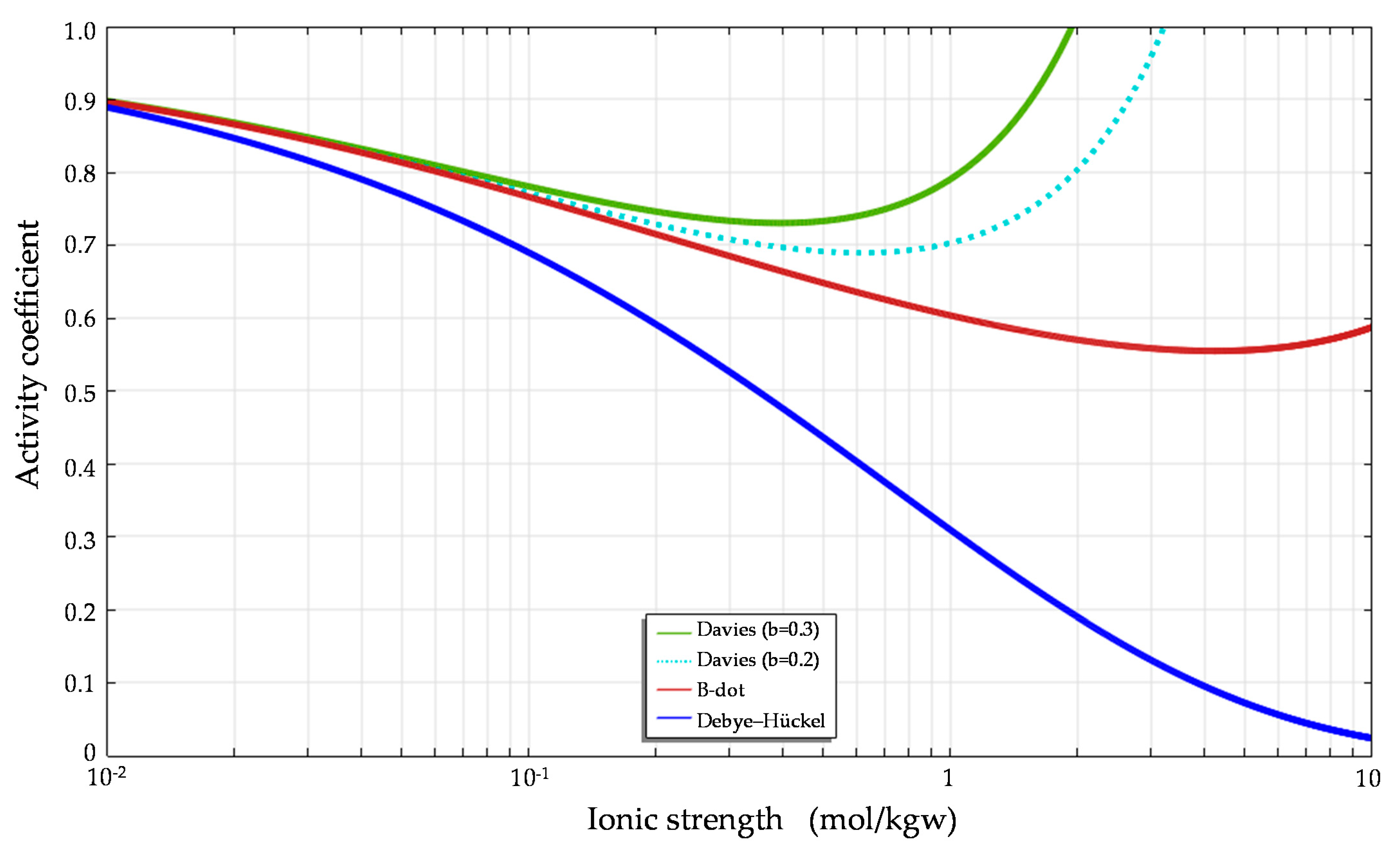
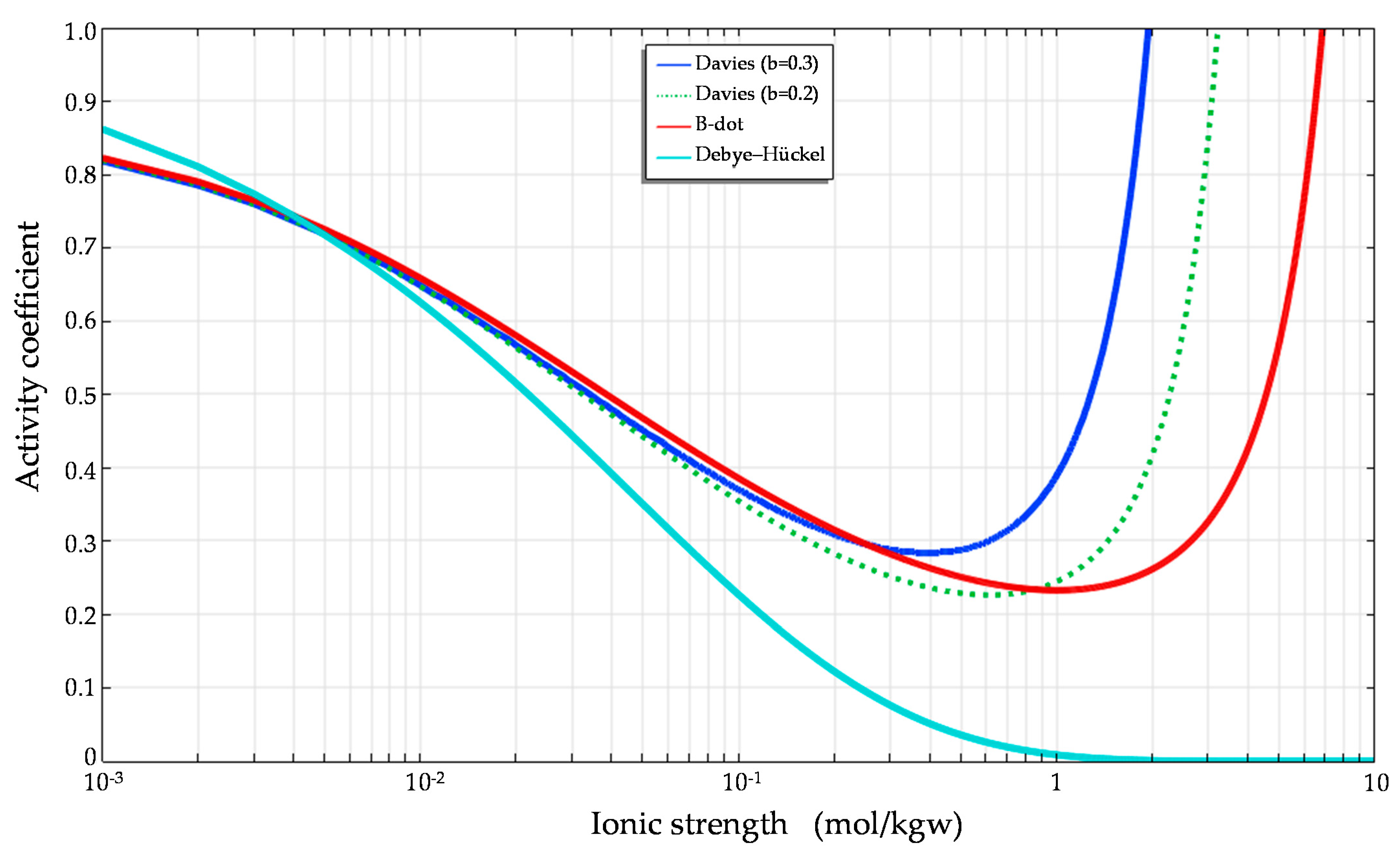
Considering the effect of short-range interactions between ions and hydration reactions, the Davies model and modified Debye–Hückel (B-dot) model derived using polynomials of ionic strength can predict activity coefficients more precisely than the Debye–Hückel model when the ionic strength increases (Figure 1 and Figure 2).

Comparisons of the activity coefficients for Ca²⁺ and Cl⁻ with ionic strength (CaCl₂ solution, a_i = 4.86 for Ca²⁺, a_i = 3.71 for Cl⁻ [13]) are shown in Figure 1 and Figure 2, respectively. The figures demonstrate the substantial differences in the activity coefficients calculated for calcium and chloride based on the Debye–Hückel, Davies and B-dot models. The predictions clearly show that different ions have different activity coefficients at the same ionic strength.

3. Pitzer equation

The Pitzer Equation [14], developed for deriving the excess Gibbs free energy of electrolytic solutions, combines the Debye–Hückel equation with additional terms in the form of a virial equation, and it is widely used in geochemistry to model systems of mixed or single strong electrolytes at high concentrations, such as seawater.

$$\begin{array}{l}\ln {\gamma }_{\pm }=-\left|{\mathrm{Z}}_M{\mathrm{Z}}_X\right|f^{\gamma }\\ +m\left(\frac{2{\nu }_M{\nu }_X}{{\nu }_M+{\nu }_X}\right)B_{MX}^{\gamma }+m^2\times \frac{2{\left({\nu }_M{\nu }_X\right)}^{\frac{3}{2}}}{{\nu }_M+{\nu }_X}{C}_{MX}^{\gamma }\end{array}$$

(13)

where ${\gamma }_{\pm }$ is the mean activity coefficient; ν_M and ν_X are the numbers of M and X ions in the formula, respectively; Z_M and Z_X are their respective charges in electronic units; and m is the molality. The other quantities are defined as follows:

$$f^{\gamma }=-A_{\varphi }\left[\frac{{\mathrm{I}}^{\frac{1}{2}}}{1+b{\mathrm{I}}^{\frac{1}{2}}}+\frac{2\ln (1+b{\mathrm{I}}^{\frac{1}{2}})}{b}\right]$$

(14)

where A_ϕ is the Debye–Hückel coefficient for the osmotic function, $B_{MX}^{\gamma }$ is the second virial coefficient, and $C_{MX}^{\gamma }$ is the third virial coefficient.

When a radioactive waste repository is in a brackish water area, the surrounding groundwater can have a high ionic strength. If the concentration of a high-salinity groundwater quality is obtained by laboratory analysis, it can be difficult to determine the real reaction concentration values of the groundwater quality due to the chemical interactions among all of the relevant ion species. The interaction among the ionic species in groundwater is related to the concentrations of the cations and anions in the aqueous solution, and the charge of each species. Therefore, it is necessary to analyze the influence of the ionic strength and the activity coefficients on the activity of the chemical species. These calculations will allow for the accurate prediction of the speciation and solubility of the nuclides released from the repository to the groundwater, and the sorption capacity of the nuclides adsorbed by bentonite.

Geochemical simulation can serve as an essential tool in the support of repository performance for two main reasons. First, geochemical simulation can help identify the chemical species formed and predict the future geochemical/environmental state. Second, there can be different scenarios and geochemical processes affecting the safety of a repository. Numerical geochemical modeling offers an effective (and often the only viable) means to conduct simulations assessing the performance of radioactive waste disposal for differing scenarios and conditions. With this purpose in mind, this study reviewed the literature on geochemical models and their applications. The studies include geochemical models, the sources of thermodynamic databases (TDBs) used in models, using TDBs to simulate nuclide solubility, the ‘sufficiency’ of TDBs for surface complexation models, case studies of nuclide sorption, and the selection and application of activity coefficient equations in geochemical models. In addition, case studies were conducted, and the performance of different activity coefficient equations in the geochemical models was compared.

2. Development of Geochemical Models

Geochemical models enable the conceptualization of chemical reactions to be represented by mathematical equations, which can then be coded up as a geochemical modeling software tool. The first geochemical model was introduced by Garrels and Thompson in 1962 [15]. Garrels and Thompson established a chemical model of seawater based on the major ions present in seawater. In the 1980s, researchers studied water–rock interactions from the perspective of physical chemistry and further integrated solute transport, dispersion transport, chemical reactions and water–rock interface chemistry. A coupled model of solute transport was therefore developed. Over the last few decades, geochemical models have been developed rapidly in response to an increasing number of problems in geochemical and environmental science which require quantitative analysis and assessment. In research supporting nuclear waste disposal, geochemical models have become a crucial tool for the simulation of geochemical processes, including the formation and evolution of hydrochemical components in water–rock systems, and surface complexation between minerals and nuclides. Geochemical models can simulate many geochemical phenomena and processes, covering: (1) chemical species in water; (2) the saturation index (SI), which can be expressed as SI = log(IAP/Ksp), where IAP is the ionic activity product, and Ksp is the solubility product; (3) the mixing of more than two solutions, as well as the resulting aqueous species composition, Eh, pH, and SI; (4) dissolution (precipitation) caused by the interaction of organic and inorganic compounds; (5) reduced pressure or changes in water’s chemical composition and SI caused by boiling or the addition of a gas; (6) the rates or kinetics of geochemical reactions; and (7) water–rock interactions. Simulations of water–rock interactions can be further divided into forward and inverse modeling. Forward modeling involves the simulation of possible dissolution–precipitation, adsorption–desorption and oxidation–reduction reactions, and the prediction of the chemical species involved in the dissolution or precipitation, as well as the mass being adsorbed or desorbed by the minerals. Inverse modeling involves the simulation of the aqueous species composition and Eh and pH values in water–rock interactions.

As chemical effects are highly crucial in the closure of a high-level radioactive waste disposal site, a geochemical model can provide an effective means to calculate the formation and evolution of chemical species under long-term water–rock interactions in both the engineering and natural barriers of the repository. Such a model is usually based on the thermodynamic data of chemical reactions. The geochemical reaction is represented by mathematical equations, which can be written into a numerical model and solved using a mathematical algorithm for its compilation into computer code. The approach of the law of mass action requires the concentration of the master chemical component and thermodynamic data such as the equilibrium constant of the product species at the pressure and temperature of interest in the heterogeneous system. For the Gibbs energy minimization, a value of the standard Gibbs free energy of each chemical component is taken from the thermodynamic database and corrected to the pressure and temperature of interest, if necessary.

Amongst the most widely used geochemical models in the approach of the law of mass action are SOLINEQ.88 [16], EQ3/6 [10,17,18,19], MINEQL+ [20], MINTEQA2 [21], PHREEQC [22] and WATEQ4F [23]. The represented geochemical models for the approach of Gibbs energy minimization are GEM Selektor [24], Reaktoro [25,26], ChemApp [27] and ChemSage/FactSage [28,29]. Geochemical models can be used for the safety assessment of engineering and natural barriers in high-level radioactive geological disposal repositories, and they can serve as a research tool for the determination of water–rock interactions and the reactive chemical transport of nuclides in near and far fields. These models are mainly composed of several modules, such as input, output, iterative algorithm and chemical TDB modules. In general, the input module consists of the total concentration of the components in the initial solution as well as the solid and gas components. The output module primarily includes the equilibrium components, species concentrations and mass exchange between the aqueous solution, solid phase and gas phase. The iterative algorithm module is used to solve nonlinear equations, and it often employs the improved Newton Raphson iterative method. The database module of chemical thermodynamics includes data on the thermodynamic equilibrium constant under a standard state (25 °C, 1 atm (1 × 10⁵ Pa)), the equilibrium constant at different temperatures, the parameters required for activity coefficient calculation, and the stoichiometric factors of each species in aqueous solutions.

3. Evaluation and Application of a Thermodynamic Database (TDB) in Geochemical Models

3.1. Evaluation of a Thermodynamic Database (TDB)

The geochemical models are shipped with thermodynamic databases, and each equilibrium constant of the TDBs for a chemical reaction can be separated from the simulation model. This means that the equilibrium constant is not rigidly embedded in the simulation model. Users can easily change the equilibrium constant value and add/delete chemical reactions without affecting the code function in the database. The geochemical models used in this study (such as PHREEQC and EQ3/6) allow users to modify the equilibrium constants in input files or databases with internal consistency.

The required data of the equilibrium constant or standard Gibbs free energy can be found in the thermodynamics database of the geochemical model. We should check whether the database contains the thermodynamic and kinetic parameters of the species involved in the model. At the same time, we should focus on whether the data in the thermodynamic database have internal consistency; for example, the enthalpy of formation (${\mathsf{\Delta }}_f{H}^0$), standard Gibbs energy of formation (${\mathsf{\Delta }}_f{G}^0$), and entropy (${\mathsf{\Delta }}_f{S}^0$) for the chemical species x may come from different sources. The value (i.e., equilibrium constant or standard Gibbs free energy) of thermodynamics database may be obtained through the statistical regression analysis of experimental data at the beginning of the derivation; however, the value may not be consistent with the relationship of the formula (${\mathsf{\Delta }}_f{G}_X^0={\mathsf{\Delta }}_f{H}_X^0-T{\mathsf{\Delta }}_f{S}_X^0$). Achieving the consistency of these parameters is an important task that is still in progress in the establishment of geochemical models and chemical thermodynamics databases [30,31].

The widely used PHREEQC geochemical model already has an internal TDB. In addition to the databases in the PHREEQC, WATEQ4F and MINTEQ models, Lawrence Livermore National Laboratory in the United States developed a database of chemical thermodynamics. The database comes with EQ3/6, which can be used in the PHREEQC model. Andra/RWM, France, developed a chemical TDB named ThermoChimie-TDB [32]. To date, the format of the ThermoChimie database has been employed by other models, including PHREEQC, CHESS [33], Crunch [34] and Toughreact [35]. The compatibility of the TDBs can be extended to other models, including Medusa [36] and Geochemist’s workbench [37], according to the demand for databases. Other research institutions have also developed various chemical TDBs. Examples include the Thermochemical Database Project developed by the Nuclear Energy Agency (NEA) [38,39,40]; the Thermodynamic Reference Database (THEREDA) focusing on transuranic elements, which was developed by various German institutions [41]; Japanese JNC TDB [42]; British HATCHES [43]; Nagra/PSI chemical TDB, developed by the Swiss Radioactive Waste Management Agency [44]; and MOLDATA [45] TDB, which is under compilation by SCK.CEN at Mol (Belgium) for use in a framework of safety case development by ONDRAF/NIRAS. These TDBs have been developed to support the geochemical modeling required for the safety and performance assessment of radioactive waste repositories. Together, they provide good coverage of geochemical reaction data for the hydrogeochemical simulation of radioactive waste disposal. Three TDBs—ThermoChimie-TDB, THEREDA and NEA TDB—are described as follows.

The latest release of ThermoChimie (V10a) can be downloaded using the “Download” table. The database contains the basic major elements, numerous nuclides and toxic chemical elements. The main elements include C, N, O, F, Na, Mg, Al, Si, P, S, Cl, K, CA, Fe and Ba. The nuclides and toxic chemical elements are outlined as follows: (1) long half-life nuclides and actinide daughter nuclides over 1000 years, including C, Al, Cl, K, Ca, Mn, Fe, Ni, Se, Rb, Zr, Nb, Mo, Tc, Pd, Sn, I, Cs, Ba, Sm, Ho, Hf, Pb, Ra, Th, Pa, U, Np, Pu, Am and Cm (Be, La, Bi and Ac will be included in the future); (2) short half-life nuclides, including CO, Sr, Ag and Eu; and (3) toxic chemical elements, including B, Cr, As, Cd and Sb. The basis for the development of the ThermoChimie database includes a pH range of 5–14, the redox stability range of water, a temperature of 15–90 °C, and an ionic strength between very low (0.001 mol/kgw) and 3 mol/kgw. The data selection process must consider both temperature and ionic strength correction. In many cases, there is not enough data to perform these corrections, and strategies have been developed to overcome this limitation [32,46].

The purpose of the THEREDA chemical database is to simulate the geochemical evolution of radioactive and chemical toxic waste disposal sites. In the process of modeling, it is necessary to check the internal consistency of the thermodynamic data (including the adsorption data) of chemical reactions between nuclides and the surrounding rock. The built-in databases provided by different geochemical models are inconsistent, such as the activity coefficient equation used in the data generation process and the experimental data of the equilibrium constant. Therefore, using different chemical databases to compare geochemical simulation results may have different results. This is due to the incomplete and conflicting data in the existing chemical databases, the different validities of the solution composition (ionic strength) and model limitations, and the lack of sorption data. THEREDA is a collaborative project that has addressed these challenges. The aim of the project is to establish a consistent and quality-assured database for all of the safety-relevant nuclide and toxic element, temperature and pressure ranges, with a focus on high-concentration brine systems. The database uses the Pitzer equation to calculate the activity coefficient applicable to such conditions. The chemical elements and nuclides in the THEREDA database are as follows: H, C, O, Na, Mg, Al, Si, P, S, Cl, K, Ca, Se, Sr, Tc, Cs, Nd, Th, U, Np, Pu, Am and Cm. Part of the THEREDA project involves the collection and evaluation of uranium chemical reaction data. The aquatic chemical and thermodynamic conditions for U (VI) and U (IV) are crucial for the geochemical modeling of disposal-site-relevant systems. The THEREDA chemical database established the correction of the activity coefficients for U, Na, K, Mg, CA, Cl, S, and C in high-salinity aqueous solutions using the Pitzer equation. The THEREDA database does not have the same strict quality requirements for thermodynamic data as the NEA TDB. Currently, THEREDA is jointly planned, implemented and further developed by the research institute engaged in the final disposal of radioactive waste and its potential host rock [41].

The NEA TDB has provided high-quality and accurate chemical thermodynamic data used in the safety assessment of deep geological repositories for the international radioactive waste management community. The scenario analysis and assessment of radionuclide migration paths to the environment are essential for the performance assessment of geological disposal. The safety assessment of radioactive waste disposal is based on the use of a chemical thermodynamics database for the numerical simulation of the speciation. The NEA mentioned [47] that their TDB has become the worldwide standard for geochemical modeling in the field of geological disposal. However, the applicability of the NEA TDB data is limited to low-to-medium ionic strength environments and temperatures of less than 100 °C. Additionally, the NEA TDB data do not cover all of the species and thermodynamic quantities required for safety assessment. Therefore, for application to natural environmental systems, users may need to obtain data from other thermodynamic databases; however, it is necessary to ensure that the selected end states are consistent and represent the chemical reactions of the system of interest. The chemical elements and nuclides in the NEA TDB are as follows: H, B, C, N, O, F, Na, Mg, Al, Si, P, S, Cl, K, Ca, Cr, Mn, Fe, Co, Ni, Cu, Zn, Ga, Ge, As, Se, Br, Rb, Sr, Zr, Tc, Ag, Cd, In, Sn, Te, I, Cs, Ba, Hg, Tl, Pb, Th, U, Np, Pu and Am. The NEA TDB has the following characteristics: a comprehensive literature review and detailed discussion of the performed evaluation; the traceability of all used the documents used in the evaluation and selection of the data; strict guidelines and a strengthened selection of high-quality values; and thermodynamic values conform to the CODATA standards [31,48,49].

3.2. Radionuclide Speciation and Solubility

The radionuclides selected for the geochemical simulation were Thorium-232, Neptunium-237 and Plutonium-242, which have a long half-life and are safety-relevant materials for radioactive waste in Taiwan. We referred to the test calculations from THEREDA [50] and used the thermodynamic database (THEREDA_PIT_PHRC_R-07.dat) to simulate the radionuclide speciation and solubility for the solid compounds Th(OH)₄, Np(OH)₄ and Pu(OH)₄ in NaCl, CaCl₂, Na₂CO₃ and KHCO₃ aqueous solution conditions (

Table 1. Initial conditions of the aqueous solution for the speciation and solubility calculation of Th(OH)_4(s).

Solution No.	Solid Compound	NaCl (mol/kgw)	CaCl2 (mol/kgw)	pH	pe	HCl (mol/kgw)	NaOH (mol/kgw)	Na2CO3 (mol/kgw)
1	Th(OH)4(s)	4.0		6.72	4.0	10−4
2	Th(OH)4(s)	4.0		6.72	4.0		10−5
3	Th(OH)4(s)		5.26	5.38	4.0		0.0010
4	Th(OH)4(s)		5.26	5.38	4.0		0.0175
5	Th(OH)4(s)			7.00	4.0		0.1	0.25
6	Th(OH)4(s)			7.00	4.0		0.1	1

,

Table 2. Initial conditions of the aqueous solution for the speciation and solubility calculation of Np(OH)_4(s).

Solution No.	Solid Compound	NaCl (mol/kgw)	CaCl2 (mol/kgw)	pH	pe	HCl (mol/kgw)	NaOH (mol/kgw)	KHCO3 (mol/kgw)
7	Np(OH)4(s)	4.0		6.72	−5.0	2 × 10−4
8	Np(OH)4(s)	4.0		6.72	−5.0		10−5
9	Np(OH)4(s)		5.26	5.38	−5.0		0.0010
10	Np(OH)4(s)		5.26	5.38	−5.0		0.04
11	Np(OH)4(s)			7.00	−5.0			0.03
12	Np(OH)4(s)			7.00	−5.0			0.3

and

Table 3. Initial conditions of the aqueous solution for the speciation and solubility calculation of Pu(OH)_4(s).

Solution No.	Solid Compound	NaCl (mol/kgw)	CaCl2 (mol/kgw)	pH	pe	HCl (mol/kgw)	NaOH (mol/kgw)	KHCO3 (mol/kgw)
13	Pu(OH)4(s)	4.0		6.72	4.0	2 × 10−4
14	Pu(OH)4(s)	4.0		6.72	4.0		10−5
15	Pu(OH)4(s)		5.26	5.38	4.0		0.0010
16	Pu(OH)4(s)		5.26	5.38	4.0		0.05
17	Pu(OH)4(s)			7.00	4.0			0.03
18	Pu(OH)4(s)			7.00	4.0			0.3

) [50] using the PHREEQC model. Additionally, we also used the PHREEQC model, and used the NEA TDB (NEA_TDB_phreeqc_Nov2018.dat) to simulate radionuclide speciation and solubility for the solid compounds Th(OH)₄, Np(OH)₄ and Pu(OH)₄ in the groundwater (

Table 4. Groundwater quality in potential radioactive waste disposal sites in Taiwan.

Component	Water Quality (mol/L)
pH	8.6
pe	−5.73
T	30.87 °C
C	1.21 × 10−3
Ca	3.76 × 10−4
Mg	6.38 × 10−5
Na	1.57 × 10−3
K	9.22 × 10−5
Fe	7.62 × 10−6
Si	8.31 × 10−4
Cl	9.77 × 10−4
S	1.05 × 10−4
N	3.35 × 10−5

) of subsurface systems of potential radioactive waste disposal sites in Taiwan.

The simulation results showed that the main dissolved ions of Th(OH)_4(s) are Th⁴⁺_(aq) and Th(OH)_4(aq), and the total dissolved concentration of Th⁴⁺ can vary with the pH, as shown in Figure 3. The main dissolved ions of NpCl³⁺_(aq), Np(OH)³⁺_(aq), Np(OH)₂²⁺_(aq), Np(OH)₃⁺_(aq), Np(OH)_4(aq) and Np⁴⁺_(aq) have a valence of 4, and the redox formations NpO₂⁺_(aq), NpO₂(OH)_(aq) and NpO₂(OH)₂⁻_(aq) have a valence of 5. The total dissolved concentration of Np⁴⁺ in relation to the pH is shown in Figure 4. The main dissolved ions of Pu(OH)_4(s) are PuCl³⁺_(aq), Pu(OH)_4(aq), Pu(OH)₃⁺_(aq), Pu(OH)₂²⁺_(aq), Pu(OH)³⁺_(aq) and Pu⁴⁺_(aq). The total dissolved concentration of Pu⁴⁺ also varied with the pH (Figure 5). There are 16 aqueous complexation formations for Th(OH)_4(s), 30 aqueous complexation formations for Np(OH)_4(s), and 24 aqueous complexation formations for Pu(OH)_4(s) in the dissolution reaction of a solid compound. Figure 6 showed the total dissolved concentrations of the solid compounds Th(OH)₄, Np(OH)₄ and Pu(OH)₄, as calculated using the groundwater quality of a potential radioactive waste disposal site in Taiwan, which can be used as the initial concentration data of radionuclides in the adsorption/desorption interactions of surface complexation reactions between nuclides and bentonite after its release from the waste canister to the engineer barrier.

4. Thermodynamic Data of the Surface Complexation Model and Case Study

4.1. Evaluation of the Thermodynamic Data for the Surface Complexation

The thermodynamic data of SCM can be used by geochemical and reactive transport models to evaluate and compare the composition and concentration of radionuclides in water and minerals in geochemical reactions in various hydrogeochemical environments. Bradbury et al. [51] proposed a surface complexation model to simulate radionuclide adsorption in natural systems. They indicated that the results of experimental methods, such as distribution coefficients (Kd) and isothermal equations, are valid only under experimental measurement conditions, and that the application of such results to other conditions and systems may be problematic. Additionally, they studied the diffuse double-layer model to describe the adsorption of radionuclides by igneous minerals. They reported that surface complexation adsorption, the development of a conceptual model, and the use of a prediction model constitute a feasible method for the scenario analysis of the safety assessment of geochemical reactions in radioactive waste environments. This method can be used under the environmental conditions of disposal sites (varying pH, Eh, and ionic composition of the surrounding water). Surface complexation models can provide reliable results for safety assessments in radioactive waste disposal.

The Nuclear Energy Agency of the Organization for Economic Co-operation and Development has regularly discussed and studied geochemical reactions concerning the surface complexation adsorption of nuclides. The agency has executed such discussions and studies in collaboration with research organizations such as ANDRA and IPSN, France; BNFL and NIREX, the United Kingdom; ENRESA, Spain; KAERI, Korea; NAGRA, Switzerland; ONDRAF/NIRAS, Belgium; JNC, Japan; POSIVA, Finland; PSI, Switzerland; SKB and SKI, Sweden; and RAWRA, Czech Republic. The Kd value of such reactions is estimated and used in the safety and performance assessment of radioactive waste disposal sites [52].

4.2. Application of Thermodynamic Data in SCM

The total dissolved concentration of Np⁴⁺ (Figure 2) was used as the concentration of the nuclide released from the waste disposal site. PHREEQC was used to simulate the surface complexation reaction of the neptunium-237 radionuclide on montmorillonite for the groundwater quality (Table 4) in the subsurface system of the potential disposal site in Taiwan. MX-80 bentonite is a buffer material used in radioactive waste disposal facilities; it is composed of 65–75% montmorillonite. Bradbury et al. [53] developed equilibrium constants for the surface complexation reactions of the sorption of Np⁴⁺ nuclides on MX-80 bentonite (

Table 5. Equilibrium constant of the surface complexation reaction for Np⁴⁺ nuclide sorption on MX-80 bentonite.

Species	log K on Strong Site
≡SsONp3+	8.5 (8.2–8.9)
≡SsONpOH2+	8.3 (8.1–8.8)
≡SsONp(OH)2+	5.5 (5.3–5.8)
≡SsONp(OH)3	0.1 (−0.032–0.21)

). The equilibrium constants of these surface complexation reactions were used as the parameters of the chemical reactions in this study. No currently available database contains the SCM parameters that are defined in the NEA TDB (NEA_TDB_ phreeqc_Nov2018.dat) that we used in the PHREEQC modeling.

Therefore, the thermodynamic data for Np nuclide adsorption to montmorillonite (Table 5) were included in the input file of the PHREEQC. With a complete database of chemical thermodynamics, we can use the PHREEQC to simulate the complexation reaction of Np⁴⁺ nuclide sorption on montmorillonite and other geochemical reactions for the groundwater quality of the potential disposal site in Taiwan.

The results showed that neptunium with a valence of 3 forms various chemical species due to redox reactions. However, there was no solid nuclide precipitation, only nuclide adsorption on montmorillonite. Neptunium with a valence of 3 forms trivalent, tetravalent, pentavalent and hexavalent ions. The main dissolved ions are as follows: trivalent neptunium, i.e., Np(CO₃)₃³⁻, NpOH²⁺, and Np³⁺; tetravalent neptunium, i.e., Np(OH)₄, Np(CO₃)₄⁴⁻, Np(OH)₂²⁺, Np(CO₃)₅⁶⁻, NpOH³⁺, NpSO₄²⁺, Np(SO₄)₂, Np⁴⁺, NpCl³⁺ and NpNO₃³⁺; pentavalent neptunium, i.e., NpO₂CO₃⁻, NpO₂⁺, NpO₂(CO₃)₂³⁻, NpO₂OH, NpO₂SO₄⁻, NpO₂(CO₃)₂OH⁴⁻, NpO₂(OH)₂⁻, and NpO₂(CO₃)₃⁵⁻; and hexavalent neptunium, i.e., NpO₂(CO₃)₂²⁻, NpO₂(CO₃)₃⁴⁻, NpO₂CO₃, NpO₂OH⁺, NpO₂²⁺, NpO₂SO₄, NpO₂Cl⁺, NpO₂(SO₄)₂²⁻, (NpO₂)₂CO₃(OH)₃^-, (NpO₂)₂(OH)₂²⁺, (NpO₂)₃(OH)₅⁺ and (NpO₂)₃(CO₃)₆⁶⁻. The results also showed that the value of Kd is 36.7 cm³/g at a pH of 8.996 and a pe of 4.068 according to the adsorption capacity of the surface complexation reaction and the total dissolved concentration (

Table 6. Adsorption capacity, total adsorption capacity, total dissolved concentration and calculated Kd for neptunium in SCM.

Sorbed Nuclide	Adsorption Capacity (mole/g Mont.)	Total Adsorption Capacity (mole/g Mont.)	Total Adsorption Capacity (mole/g Bentonite)	Total Dissolved Concentration (mol/L)	Kd (cm3/g)
Mon_sONp(OH)3	4.206 × 10−11	4.21 × 10−11	2.74 × 10−11–3.16 × 10−11 (65–75% montmorillonite)	9.582 × 10−10	28.6–33
Mon_sONp(OH)2+	1.067 × 10−14
Mon_sONpOH2+	6.805 × 10−21
Mon_sONp3+	1.090 × 10−29

).

5. Different Activity Coefficient Equations in Geochemical Models

Following groundwater invasion into a deep geological repository, radioactive species are released and react with hydrogeological materials. Considering the ion interactions occurring in the in-situ chemical reactions, an activity coefficient is used to modify the chemical activities to represent the real concentration of the generated species.

Four chemical equilibrium models, namely PHREEQC, MINEQL+, MINTEQA2 and EQ3/6, were used to test the model’s applicability. The results can provide a general guideline for the selection of an appropriate model in field assessments.

5.1. Geochemical Equilibrium Models

Modeling the chemical equilibrium of target compounds is relevant during the control of pH, alkalinity, temperature and other factors. As part of this approach, one must determine the rates of the contribution of various components with specific chemical characteristics to mixtures. A model established using thermodynamic equilibrium theory and experimental data is suitable for the probing of the reaction of geochemical equilibrium; furthermore, the model can present the reaction process in a natural environment in numerical form. With extensive theoretical research and experimental data analyses on geochemical reactions, geochemical equilibrium models have become increasingly reliable for the simulation of in situ subsurface water–rock interactions and the prediction of solution concentrations through mineral ingredient analysis. Thermodynamic chemical equilibrium typically aims at the determination of spontaneous changes to an equilibrium state. Any system that is not at equilibrium would change spontaneously with the release of energy. In general, simulation is more straightforward for a closed system than an open system, in which the equilibrium condition is simplified with mass balance and thermodynamic equilibrium. This study compared the performance of four chemical equilibrium models, namely PHREEQC, MINEQL+, MINTEQA2, and EQ3/6, in terms of the prediction of activity coefficients.

5.1.1. PHREEQC Model

PHREEQCI is a complete windows-based graphical user interface to the geochemical computer program PHREEQC developed by the U.S. Geological Survey, and it provides all of the capabilities of the geochemical model PHREEQC, including speciation, batch-reaction, 1D reactive-transport and inverse modeling [22].

5.1.2. MINEQL+ Model

MINEQL+ is a chemical equilibrium model capable of calculating aqueous speciation, solid phase saturation states, precipitation–dissolution and adsorption. An extensive thermodynamic database is included in the model [20].

5.1.3. MINEQA2 Model

MINEQA2 was originally developed by Battelle Pacific Northwest Laboratory in the mid-1980s as MINTEQ. MINTEQA2 was derived from MINTEQ. MINTEQA2 is a chemical equilibrium model for dilute solutions with ionic strengths up to about 0.5 m. The model is useful for the calculation of the equilibrium mass distribution among dissolved species, adsorbed species and multiple solid phases under a variety of conditions, including a gas phase with constant partial pressures. A comprehensive database is included, which is adequate for solving a broad range of problems without the need for additional user-supplied equilibrium constants [21].

5.1.4. EQ3/6 Model

In the mid-1970s, the EQ3/6 software package was developed at Northwestern University to model seawater–basalt interactions in mid-ocean ridge hydrothermal systems. The EQ3/6 contains two kinds of calculations for aqueous solutions and aqueous systems. The first kind is called a speciation–solubility calculation, which describes the chemical and thermodynamic state of the solution using input analytical data and theoretical assumptions. The second kind of calculation is called a reaction path calculation. A reaction path calculation predicts the evolution of a reacting system [18,19].

The four chemical equilibrium models provided several equations relevant to activity coefficient calculation (

Table 7. Options of activity coefficient equations incorporated with four models.

	Davies	Modified Debye-Hückel	Pitzer
PHREEQC	v	v	v
MINEQL+	v
MINTEQA2	v
EQ3/6	v	v	v

).

5.2. Model Calibration

According to the analysis by Nordstorm et al. [54], the simulation of different chemical models in the same conditions brings about different outcomes due to the different thermodynamic databases in the models. The thermodynamic database includes the equilibrium constant, heat constant and stoichiometry. In the database of the geochemical model, there are chemical species that are mathematically independent, which are generally called chemical components. The chemical components in the database of the geochemical model are the main cation and anion species of in-situ water quality data. We can select these chemical components as reactants in order to calibrate the model. Thus, in order to realize the effect of the database on the chemical equilibrium model, a test case with the same concentrations of all of the reactants from the in-situ water quality data was selected as the input of the four models (

Table 8. Input parameters of the test case.

Parameter	Value
T	25 °C
pH	8.01
pe	7.436
Ca2+ (mol/kgw)	3.05 × 10−2
CO32+ (mol/kgw)	1.23 × 10−1
Cl− (mol/kgw)	2.8 × 10−2
K+ (mol/kgw)	3.6 × 10−3
Mg2+ (mol/kgw)	3.09 × 10−2
Na+ (mol/kgw)	5.2 × 10−2
SO42− (mol/kgw)	8 × 10−3
I (mol/kgw)	1.846 × 10−1

). The concentration and activity coefficients were calculated using the Davies equation with their respective thermodynamic databases (

Table 9. Thermodynamic databases used by the four chemical equilibrium models.

Chemical Equilibrium Model	Thermodynamic Database
PHREEQC	phreeqc.dat
MINEQL+	MINTEQA2
MINTEQA2	MINTEQA2
EQ3/6	COM

).

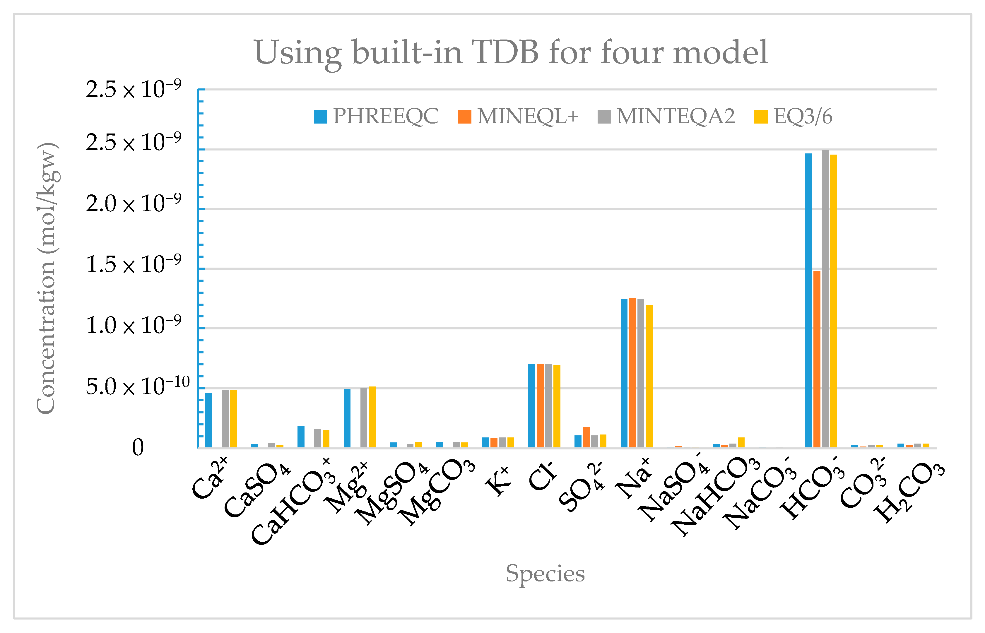
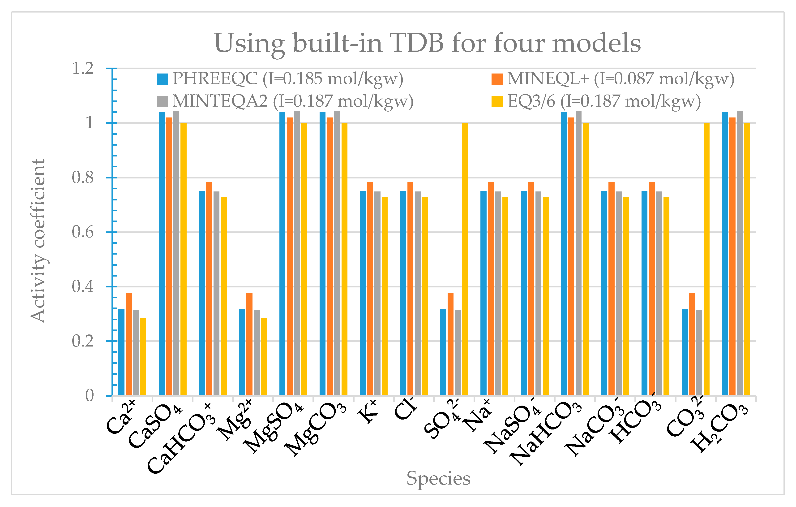
The concentration of the reaction products (Table III) and activity coefficients (Table IV) given by the four models demonstrate great differences.

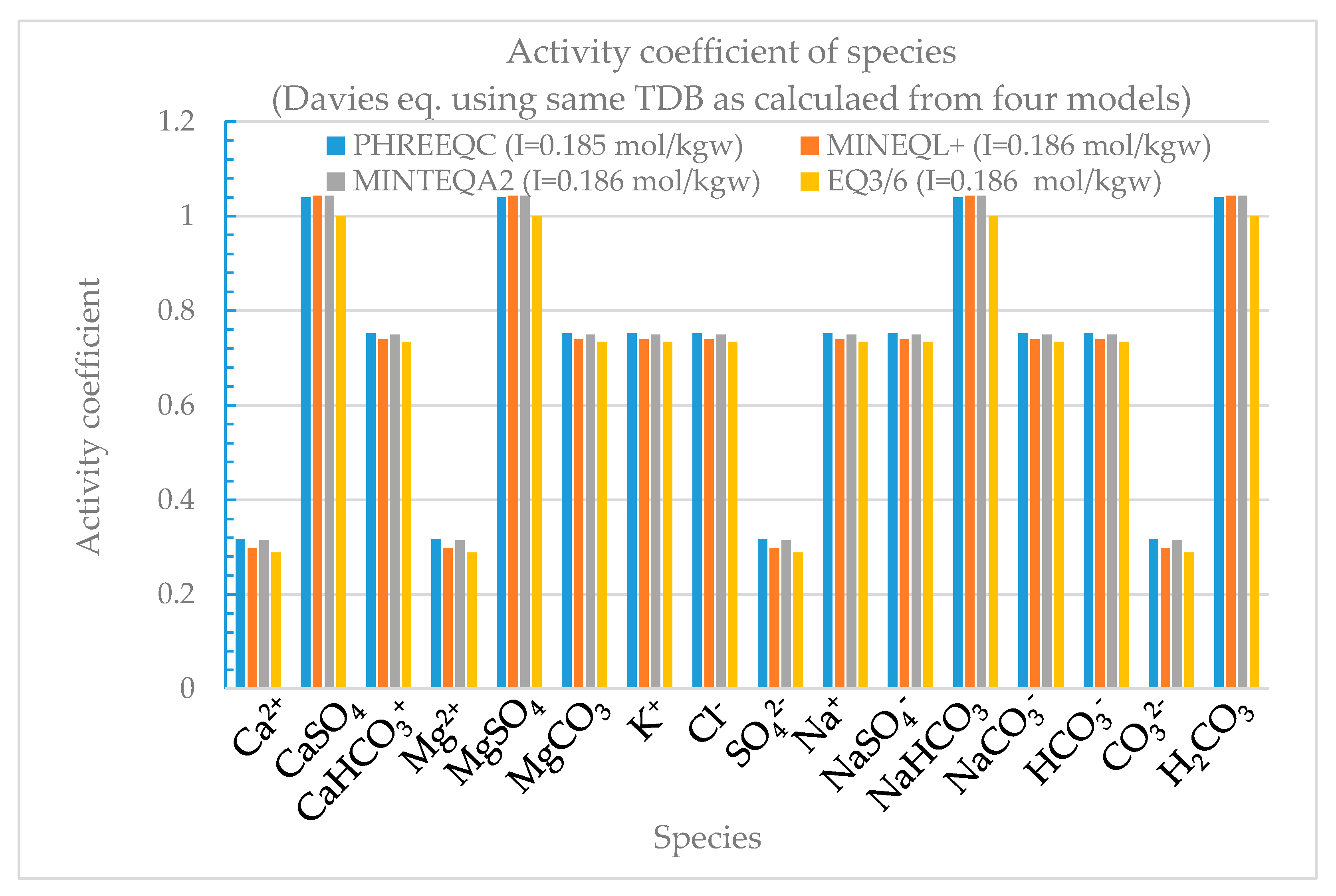
Figure 7 and Figure 8 show the concentration and activity coefficient of the major reaction products calculated by the Davies equation using the built-in thermodynamic databases of the four models, respectively. The concentrations of the reaction products and activity coefficients obtained from the four models demonstrate great inter-model differences, especially for MINEQL+. The reason for this is that MINEQL+ produces precipitation species, such as dolomite and calcite, while the saturation index (SI) values calculated by the other three model systems show that precipitation reactions do not easily occur. In order to remove the difference caused by these databases on the activity coefficients, we took the “phreeqc.dat” database of PHREEQC as the standard in order to revise the databases MINTEQA2 and COM, and recalculated new concentration of products (Figure 9) and activity coefficients (Figure 10). The results showed that only the concentrations of Na⁺, NaHCO₃ and NaCO₃⁻ in the EQ3/6 model were different from those in the other models. The reason for these differences is that there are chemical reactions of NaCl and NaOH in the COM database. These reactions were not considered in the PHREEQC and MINTEQA2 databases. Thus, the results showed that the differences of the concentration and activity coefficient between the models decreased significantly (Figure 7, Figure 8, Figure 9 and Figure 10) and assured us that the use of the same thermodynamic database can produce similar activity coefficients through the four models.

At present, there is no thermodynamic database in any geochemical model that contains all of the chemical species and reaction types of the solutions and minerals that may react. Developers cannot guarantee the internal consistency of the TDB. Recent research has focused on the determination of the optimal TDBs and the internal consistency of the data (e.g., standard Gibbs free energy) [30,31]. Thus, the main challenges and limitations of geochemical modeling would be to check the accuracy of the data in the database, the consistency of the chemical thermodynamics data, and the thermodynamic data sensitivity of the simulation using the database.

5.3. Comparison of the Activity Coefficients between the Models

This study considered various concentration levels in a solution (Ca²⁺, HCO³⁻, Cl⁻, K⁺, Mg²⁺, Na⁺, SO₄²⁻, Fe³⁺ and PO₄³⁻ were considered to be the major ions) in order to investigate the differences in the activity coefficient calculation performance between the four models (i.e., PHREEQC, MINEQL+, MINTEQA2 and EQ3/6).

The considered cases were as follows:

(1) The activity coefficient of a species calculated using the Davies equation in the four models.

(2) The activity coefficient of a species calculated using the modified Debye–Hückel equation in EQ3/6 and PHREEQC.

(3) The activity coefficient of a species calculated using the Pitzer equation in EQ3/6.

(4) Considering the effect of temperature on the activity coefficient, the activity coefficient of a species calculated using the modified Debye–Hückel and Davies equations at 10 °C, 25 °C, 60 °C and 90 °C.

Calculation Results

The results showed that if the ionic strength (I) of a solution was <0.0001 m, the activity coefficients of any species corrected using the Davies or modified Debye–Hückel equations for different charge numbers of ions (Z) were mostly greater than 0.95 (

Table 10. Activity coefficients using the Davies or modified Debye–Hückel equations for the four models.

PHREEQC, Davies Equation					MINTEQA2, Davies Equation
I, (mol/kgw)	Z = 1, Na+	Z = 2, SO42−	Z = 3, Fe3+	Z = 0	I, (mol/kgw)	Z = 1, Na+	Z = 2, SO42−	Z = 3, Fe3+	Z = 0
2.47 × 10−5	0.993	0.977	0.948	1.000	2.47 × 10−5	0.993	0.977	0.948	1.000
2.42 × 10−4	0.982	0.931	0.851	1.000	2.42 × 10−4	0.982	0.931	0.851	1.000
4.68 × 10−3	0.929	0.745	0.516	1.000	4.69 × 10−3	0.929	0.745	0.515	1.001
MINEQL+, Davies equation					EQ3/6, Davies equation
I, (mol/kgw)	Z = 1, Na+	Z = 2, SO42−	Z = 3, Fe3+	Z = 0	I, (mol/kgw)	Z = 1, Na+	Z = 2, SO42−	Z = 3, Fe3+	Z = 0
1.78 × 10−4	0.995	0.974	0.944	1.000	2.47 × 10−5	0.994	0.977	0.949	1.000
1.40 × 10−3	0.959	0.845	0.684	1.000	2.42 × 10−4	0.982	0.930	0.850	1.000
3.85 × 10−3	0.935	0.763	0.544	1.001	4.69 × 10−3	0.930	0.741	0.510	1.000
PHREEQC, modified Debye–Hückel equation					EQ3/6, modified Debye–Hückel equation
I, (mol/kgw)	Z = 1, Na+	Z = 2, SO42−	Z = 3, Fe3+	Z = 0	I, (mol/kgw)	Z = 1, Na+	Z = 2, SO42−	Z = 3, Fe3+	Z = 0
2.47 × 10−5	0.993	0.977	0.948	1.000	2.47 × 10−5	0.994	0.977	0.949	1.000
2.42 × 10−4	0.982	0.931	0.851	1.000	2.42 × 10−4	0.982	0.931	0.854	1.000
4.68 × 10−3	0.929	0.750	0.516	1.000	4.68 × 10−3	0.927	0.747	0.544	1.000

). It should be noted that except for Fe³⁺ ions with Z = 3, which are slightly less than 0.95, all other ions meet this threshold value (I < 0.0001 mol/kgw). The results suggest that the activity coefficient correction is small and can be neglected at such a low concentration level.

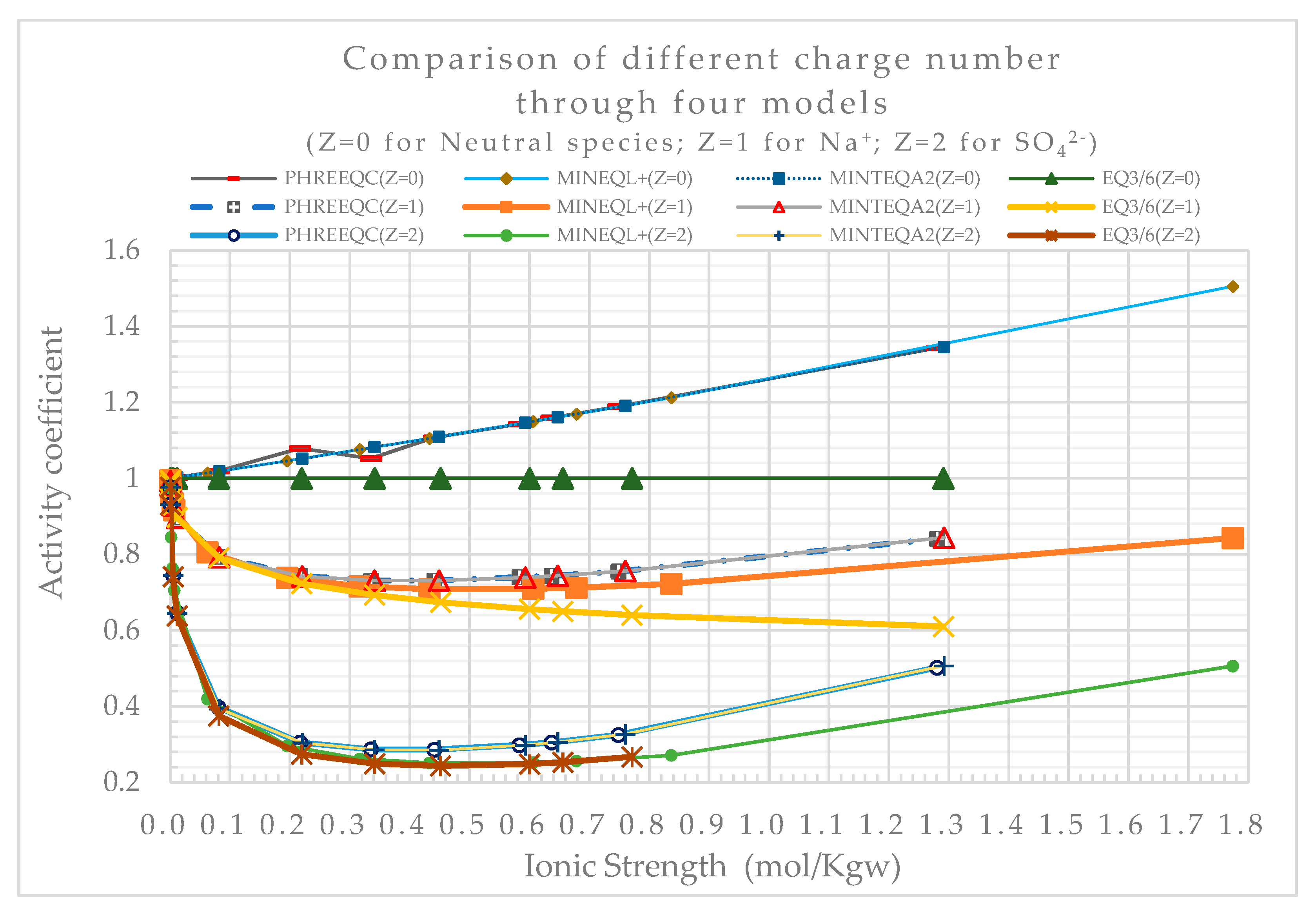
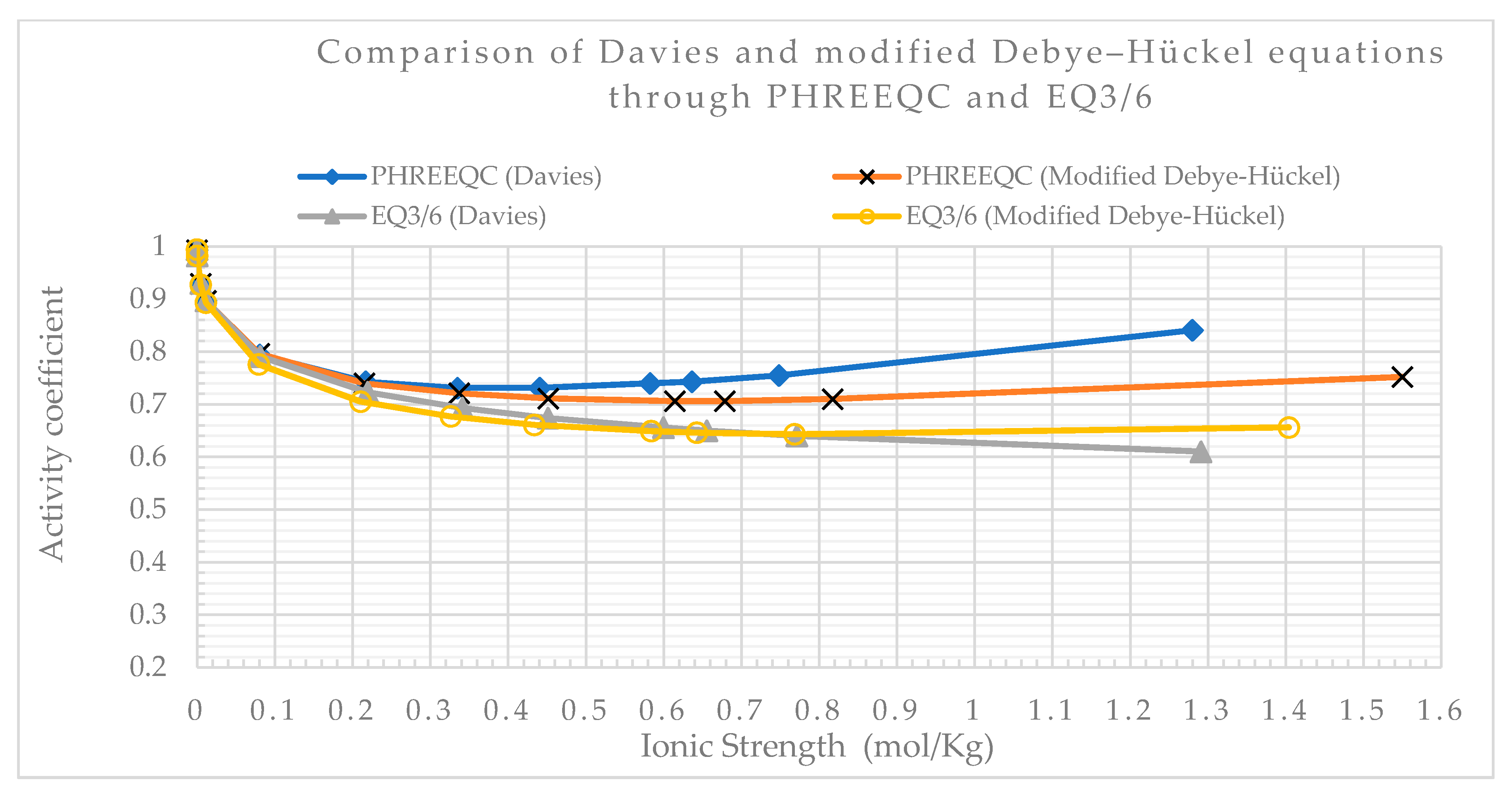
When I was <0.5 mol/kgw, the activity coefficient variation calculated using the Davies equation was <3%; as I increased from 0.5 to 0.9 mol/kgw, the maximum variation in the activity coefficient increased to about 10% (Figure 11). Therefore, the Davies equation is suitable for solutions with an ionic strength of <0.5 mol/kgw. Moreover, the activity coefficients of high-charge species calculated using the Davies or modified Debye–Hückel equations were more sensitive than those of low-charge species. 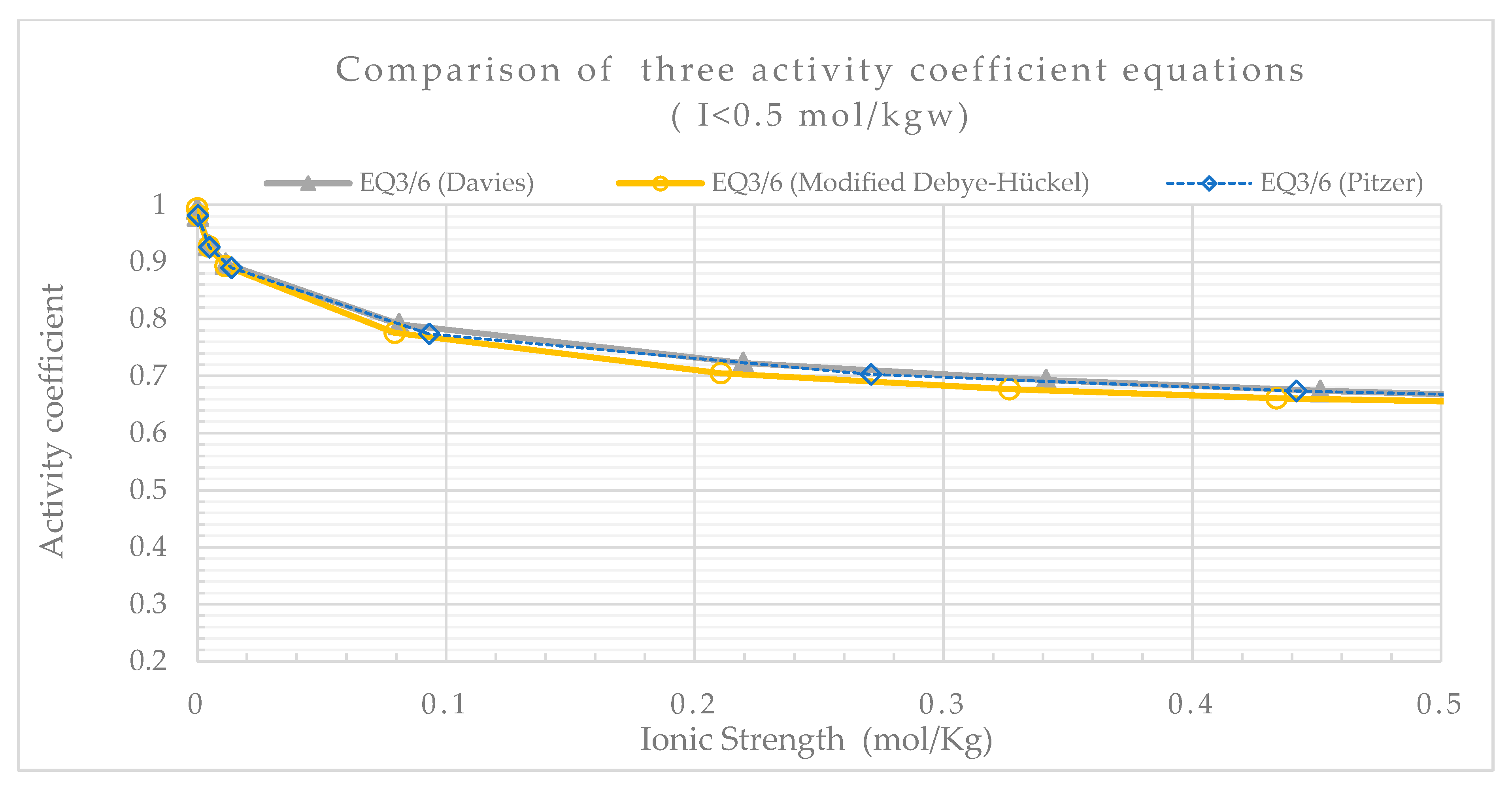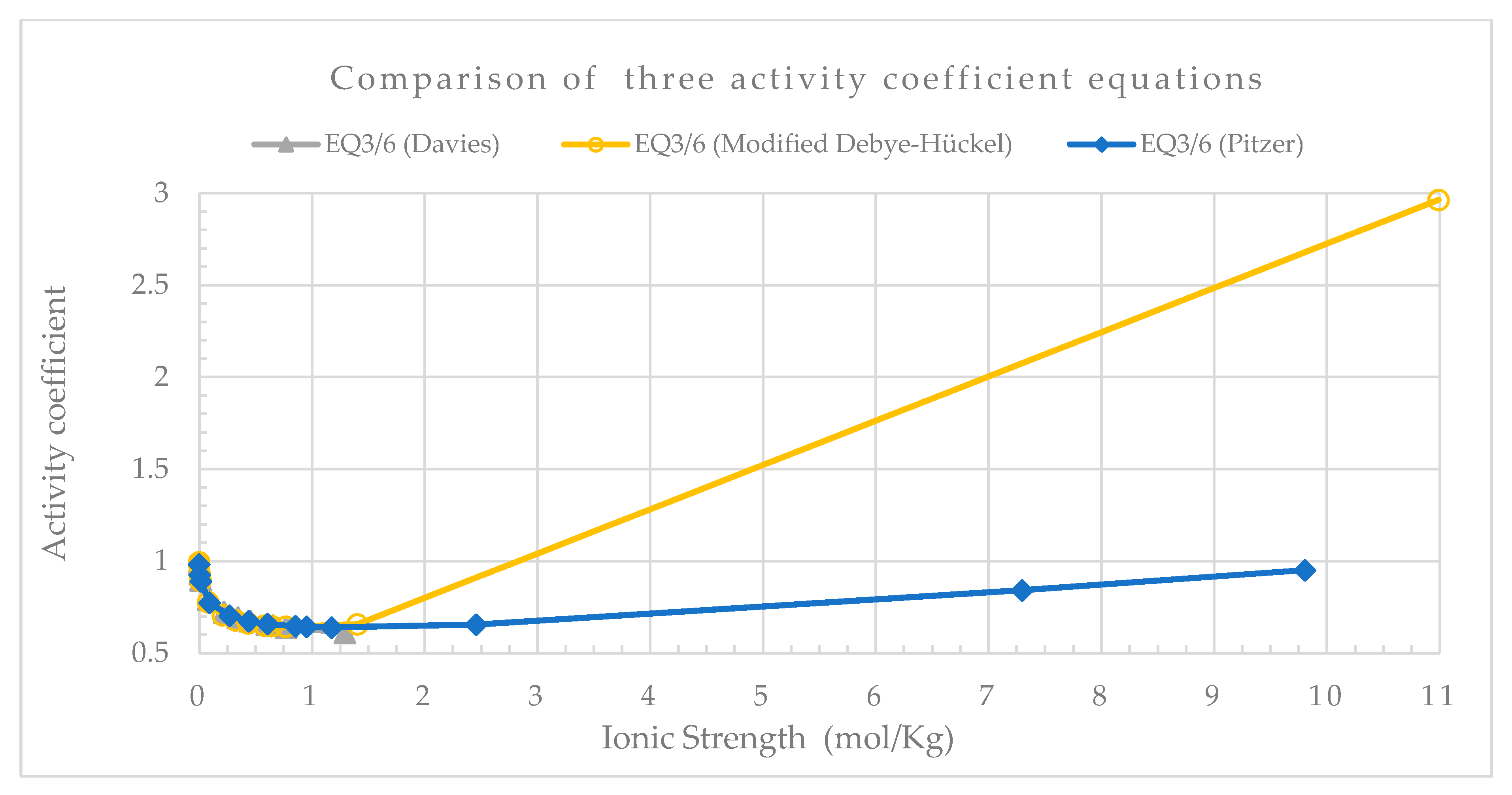Comparing the activity coefficients calculated using the Davies and modified Debye–Hückel equations through PHREEQC and EQ3/6 revealed that if I was <0.5 mol/kgw, the activity coefficient differences were <5%; if I was >0.5 mol/kgw, the activity coefficient differences increased slowly (Figure 12). According to the theory of activity coefficient, the Davies equation can be suitable for solutions with I < 0.5 mol/kgw, and the modified Debye–Hückel equation can be suitable for solutions with I between 0.3 and 1 mol/kgw. If I was <0.5 mol/kgw, the differences in activity coefficients calculated using the Pitzer, Davies and modified Debye–Hückel equations through EQ3/6 were <8%. When I was >0.5 mol/kgw, the differences increased gradually (Figure 13). 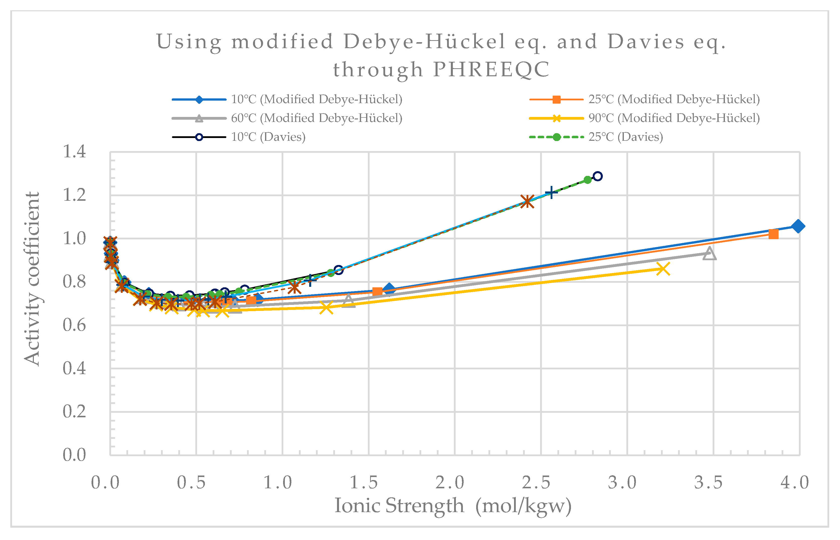Notably, the Pitzer equation described the activity coefficient satisfactorily for solutions with high ionic strength (Figure 14). As the temperature increased from 10 °C to 90 °C, the activity coefficients calculated by the PHREEQC model using the Davies and modified Debye–Hückel equations decreased. 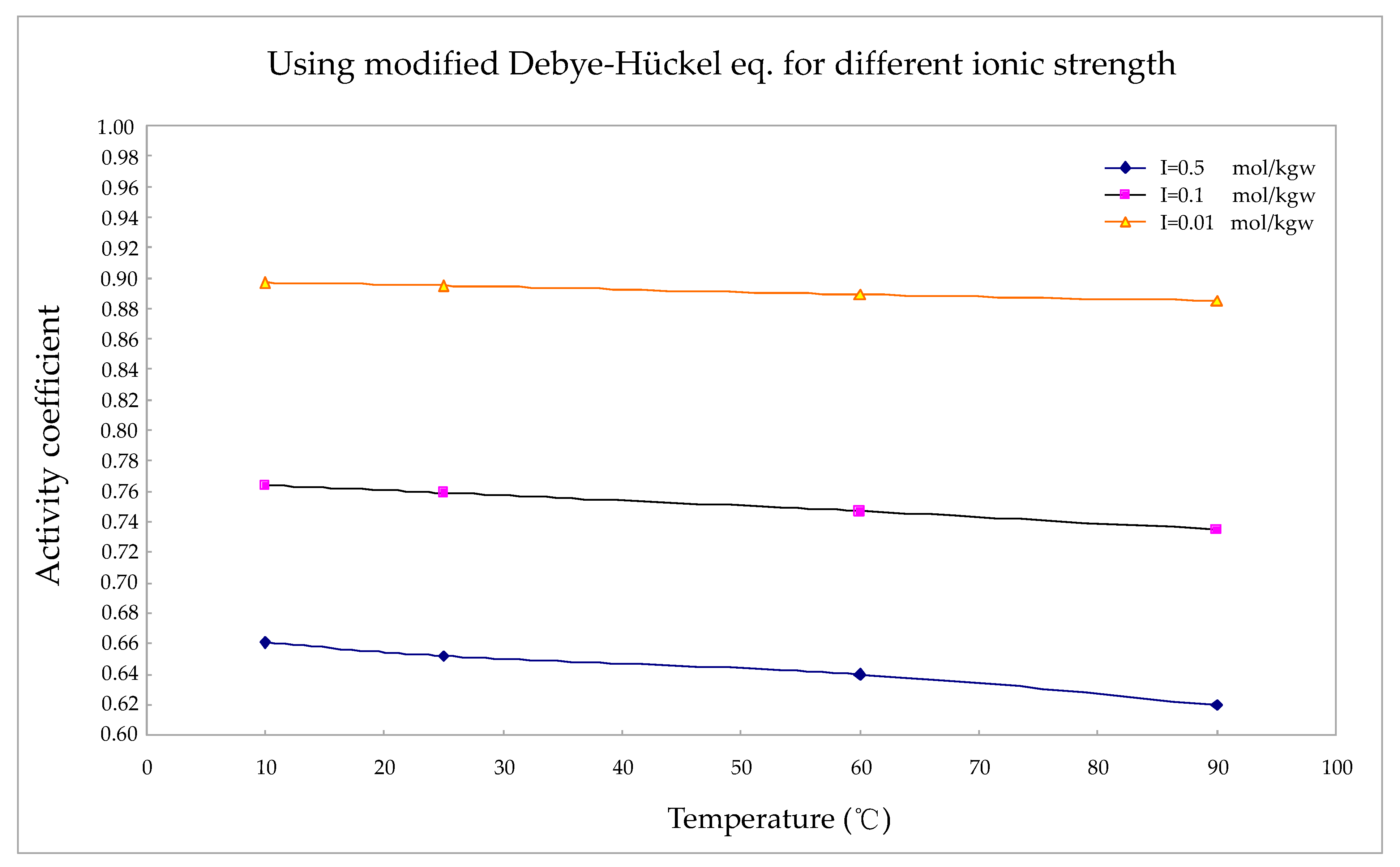Moreover, if I was <0.5 mol/kgw, the activity coefficients calculated using the Davies and modified Debye–Hückel equations were similar (Figure 15), suggesting that the Davies equation is applicable for conditions involving moderate temperature variations. The activity coefficient decreased with the increase of temperature from 10 °C to 90 °C for the modified Debye–Hückel equation, as calculated from EQ3/6 (Figure 16).

5.4. Field Applications of the Two Sites

This study also considered two field cases, namely Shiau-Chiou in Kinmen County and Bai-Shi Lake in Hsinchu County. The four models were used to calculate the activity coefficients of the solutions at these two sites.

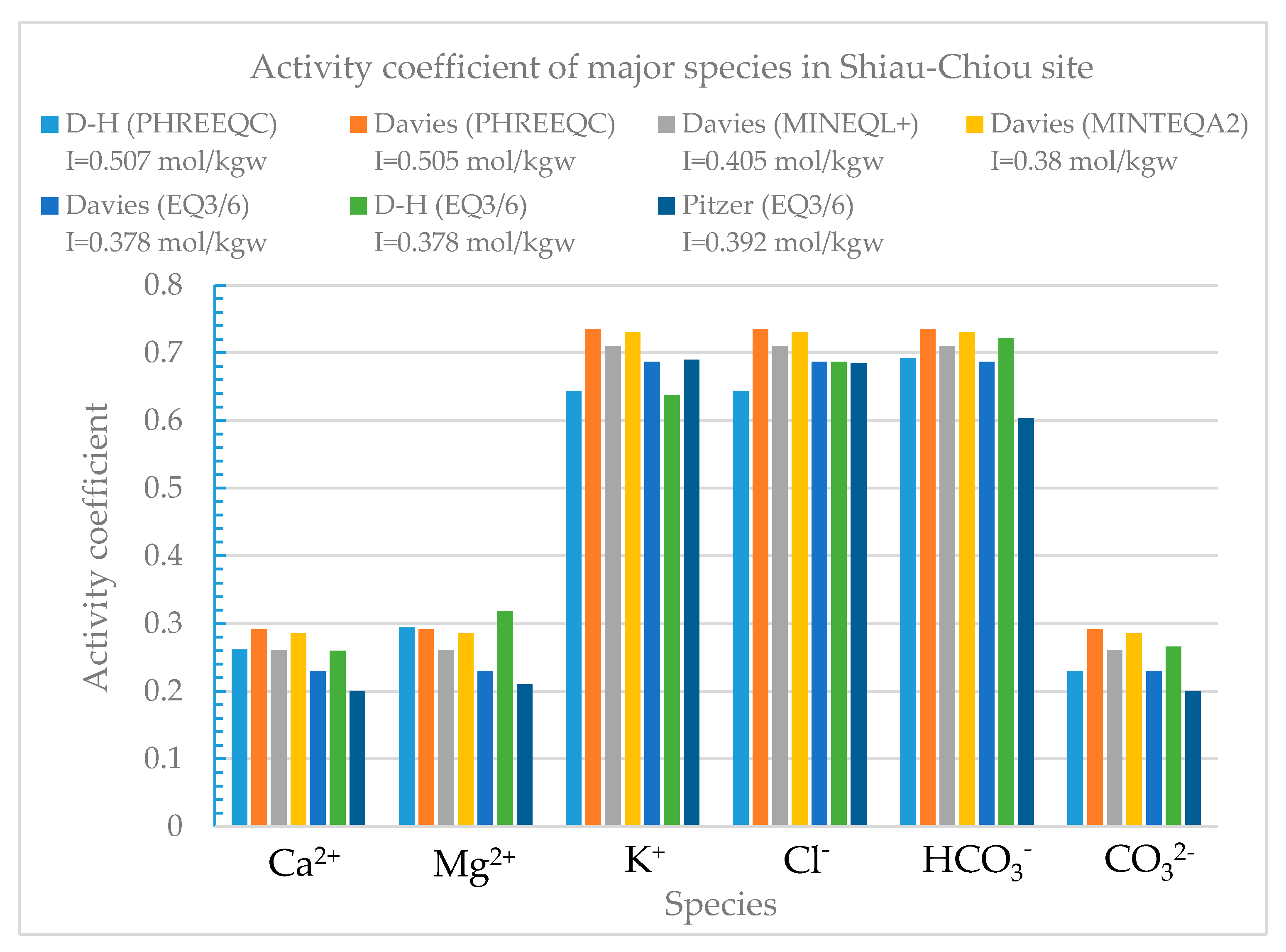
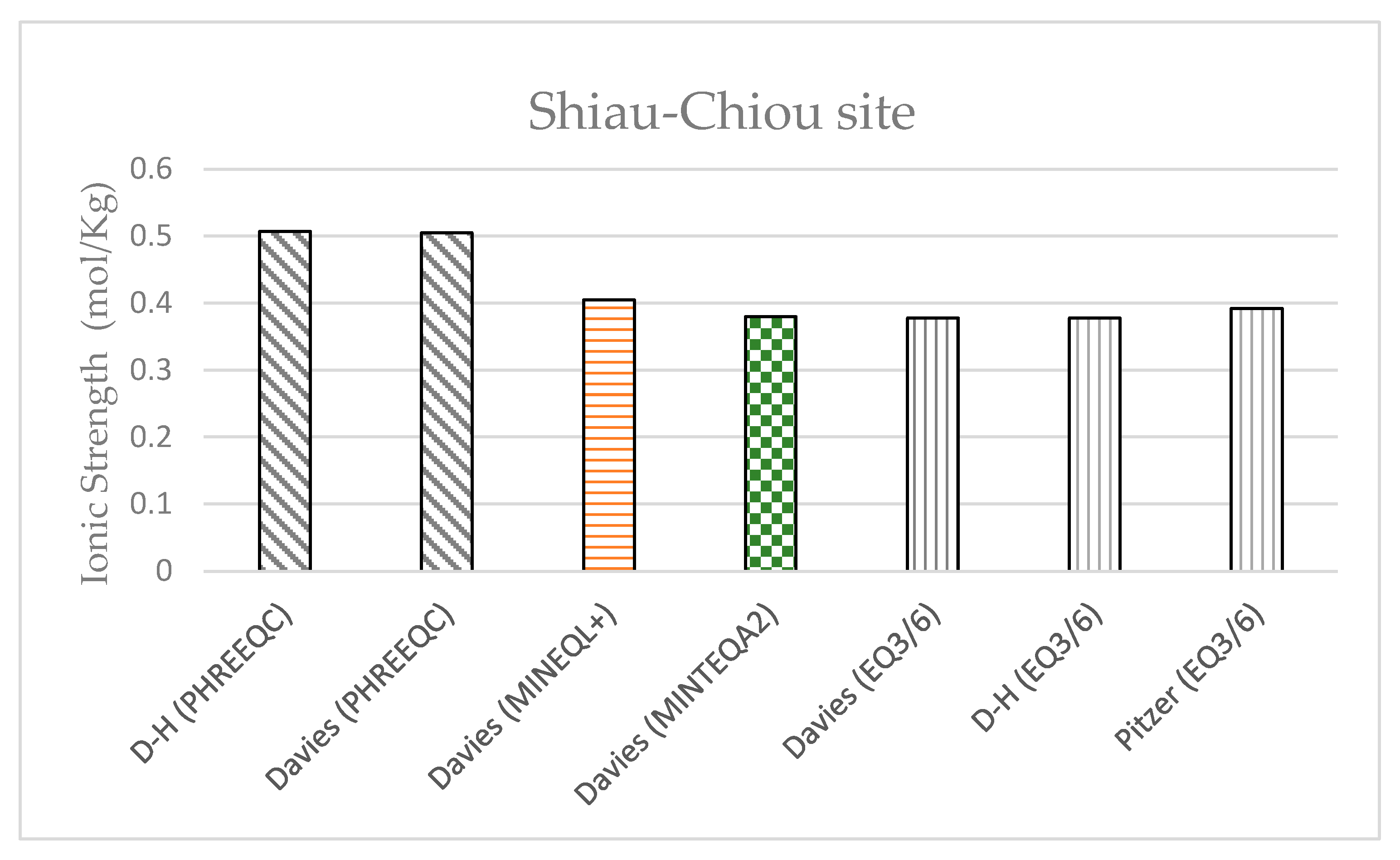
Shiau-Chiou is a possible disposal site for low-level radioactive waste in Kinmen County. The groundwater quality data measured by the Industrial Technology Research Institute (

Table 11. Groundwater quality of Shiau-Chiou, Kinmen County, and Bai-Shi Lake, Hsinchu County.

Shiau-Chiou		Bai-Shi Lake
Well depth (m)	23.20	Well depth (m)	59
Temperature (°C)	22.16	Temperature (°C)	22.2
pH	6.50	pH	8.86
pe	0.54	DO(ppm)	0.12
As	8.00 × 10−9	pe	−1.39
HCO3− (M)	5.00 × 10−4	Na+ (M)	1.9 × 10−5
CaCO3 (M)	8.33 × 10−5	K+ (M)	9.4 × 10−8
Ca2+ (M)	1.44 × 10−2	Ca2+ (M)	1.16 × 10−7
Cl+ (M)	1.69 × 10−1	Mg2+ (M)	6.46 × 10−8
Fe (M)	9.44 × 10−4	Mn2+ (M)	9.1 × 10−10
K+ (M)	4.35 × 10−3	Al3+ (M)	2.63 × 10−9
Mg2+ (M)	1.74 × 10−2	B(OH)3 (M)	1.56 × 10−7
Mn2+ (M)	3.30 × 10−4	Fe2+ (M)	7.14 × 10−10
NO2− (M)	8.70 × 10−8	Fe3+ (M)	1.07 × 10−9
NO3− (M)	3.87 × 10−6	SiO2 (M)	3.45 × 10−7
Total nitrogen (M)	3.29 × 10−5	F− (M)	9.9 × 10−8
Na+ (M)	4.57 × 10−1	Cl− (M)	5.05 × 10−7
Pb (M)	7.12 × 10−7	HCO3− (M)	9.3 × 10−6
PO43− (M)	ND	NH3 (M)	2.44 × 10−8
P (M)	ND	NO3− (M)	7.09 × 10−9
S2− (M)	1.56 × 10−7	NO2− (M)	8.7 × 10−10
SiO2 (M)	8.10 × 10−4	HPO42− (M)	1.9 × 10−8
SO42− (M)	6.94 × 10−3	HS− (M)	6.25 × 10−11
Zn2+ (M)	0	SO42− (M)	7.5 × 10−8

) were used in this study; the data were entered into the four models in order to calculate the activity coefficients of the solution ions using the Davies and modified Debye–Hückel equations. The ionic strength calculated for the groundwater samples obtained from Shiau-Chiou ranged from 0.3 to 0.5 mol/kgw (Figure 17), indicating that the Davies and modified Debye–Hückel equations can yield fairly consistent activity coefficients (Figure 18).

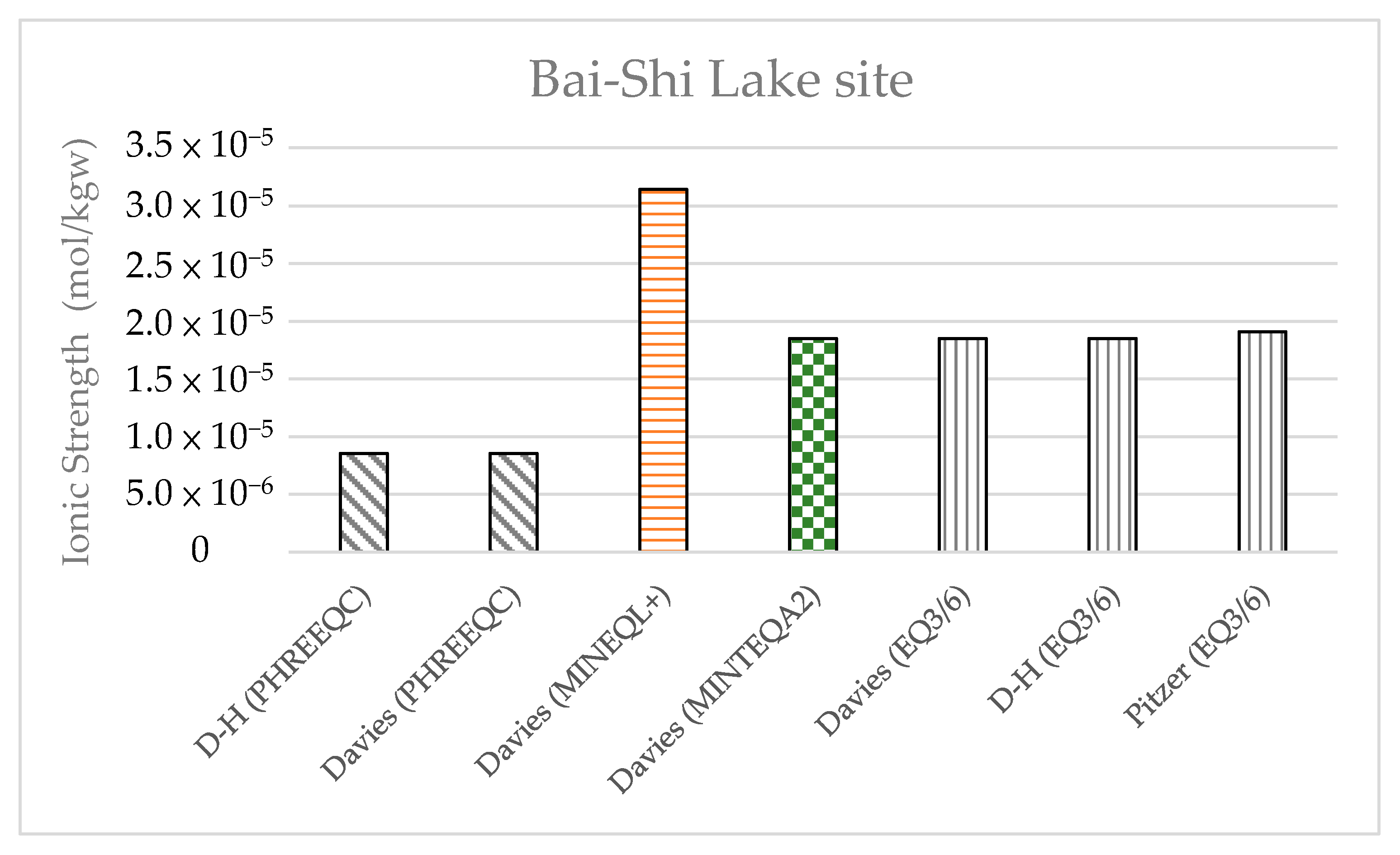
The data of the water quality obtained at Bai-Shi Lake (Table 11) were compared with those obtained at Shiau-Chiou. The results showed that the water quality at Bai-Shi Lake complied with potable water standards, whereas the groundwater at Shiau-Chiou had higher concentrations of ions, with I ranging between 0.3 and 0.5 mol/kgw. The ionic strength levels calculated at Bai-Shi Lake by the four models (Figure 19) were <10⁻⁴ m, and the activity coefficient was approximately 1, suggesting that the concentrations did not need correction through the activity coefficient models.

6. Discussion

6.1. Internal Consistency of TDBs for Supporting the Safety Assessments of Radioactive Waste Repositories

There is no internal database for PHREEQC or any other geochemical model. The different geochemical models are shipped with different thermodynamic databases. Each database is derived from different data sets or historical collections of data and experiments that possibly focus on systems with different conditions (e.g., the ionic strength and the pH of a solution, the pressure state and the temperature range), and they include different elements, minerals and ionic species. The chemical thermodynamics databases collect the values of the selected formations (Gibbs energy, enthalpy, entropy and constant pressure heat capacity), reaction data (equilibrium constant, Gibbs energy, enthalpy and reaction entropy), their uncertainty intervals, and the species and reactions in the safety assessments of radioactive waste repositories [55,56,57]. In addition, the modification of the activity coefficient by ionic strength must follow the activity coefficient equation, such as the Pitzer, Davies, modified Debye–Hückel equations, and the specific ion interaction theory (SIT) model. Thermodynamic data are collected from different data sets or experimental data. The internal consistency of a thermodynamic database must account for at least six different requirements: (1) all of the data in the database must conform to the basic thermodynamic relations and their results; (2) all of the data must be derived from a set of reference values (such as the reference temperature and pressure, the thermodynamic properties of elements and other basic compounds, etc.) and constants (such as the gas constant and molecular weight, etc.); (3) the standard state should be properly selected and suitable for all similar substances; (4) the appropriate mathematical model must be selected to fit all of the temperature and pressure data; (5) the appropriate aqueous chemical model must be selected to fit all of the aqueous solution data; and (6) all of the relevant experimental data and the data types must expressed and considered, and the conflicts and inconsistencies between the experimental measurements must be resolved [30,31].

The thermodynamic databases supporting the safety assessment of repositories may be internally inconsistent because they usually come from two or more source databases. Generally, the consistency of their internal databases can be verified through the following procedures: [31]

• Check for internal consistency

1. Formation data

The standard Gibbs energy of formation (${\mathsf{\Delta }}_f{G}_X^0$), enthalpy of formation (${\mathsf{\Delta }}_f{H}_X^0$) and entropy (${\mathsf{\Delta }}_f{S}_X^0$) for the chemical compound X are in the standard condition (T = 298.15 K). The internal consistency of the formation data for the chemical compound X is checked with the Gibbs–Helmholtz equation:

$${\mathsf{\Delta }}_f{G}_X^0={\mathsf{\Delta }}_f{H}_X^0-T{\mathsf{\Delta }}_f{S}_X^0$$

(15)

$${\mathsf{\Delta }}_f{S}_X^0=S_X^0-{\displaystyle \sum _i{\alpha }_i{S}_i^0+{\mathrm{z}}_X\frac{S_{H_{2(g)}}^0}{2}}$$

(16)

${\mathsf{\Delta }}_f{S}_X^0$. is the absolute entropy of the chemical compound X in the standard condition, ${\alpha }_i$ is the stoichiometric coefficient of the component element i in the chemical compound, $S_i^0$ is the absolute entropy of the element i divided by the stoichiometric coefficient of at standard condition, ${\mathrm{z}}_X$ is the charge of the chemical compound X in the standard condition, and $S_{H2\left(g\right)}^0/2$ is the electron entropy by convention.

For chemical compound X, the standard Gibbs energy (${\mathsf{\Delta }}_f{G}_X^0$), enthalpy (${\mathsf{\Delta }}_f{H}_X^0$), and entropy (${\mathsf{\Delta }}_f{S}_X^0$) are calculated by Equation (16). All of these values must conform to Equation (15) in the standard condition.

2. Reaction data

The relationship between the standard Gibbs energy and the equilibrium constant must conform to Equation (5) at T = 298.15 K.

• Check cross-consistency

1. The consistency between ${\mathsf{\Delta }}_r{G}_X^0$ and the ${\mathsf{\Delta }}_f{G}_X^0$ of the subject species can be expressed as:

$${\mathsf{\Delta }}_r{G}_X^0={\displaystyle \sum _{p=\mathrm{product}}{\upsilon }_P}{\mathsf{\Delta }}_f{G}_{X,P}^0-{\displaystyle \sum _{r=\mathrm{reactant}}{\upsilon }_r}{\mathsf{\Delta }}_f{G}_{X,r}^0$$

(17)

where the first and second terms are the total accumulation of all of the product species (P) and all of the reactants (r) for standard Gibbs energy, and υ_P and υ_r are the stoichiometric coefficients of the products (P) and reactants (r) involved in the reaction, respectively. The consistency in the relationship among ${\mathsf{\Delta }}_f{G}_X^0$, the product term ${\mathsf{\Delta }}_f{G}_{X,P}^0$ and the reactant term ${\mathsf{\Delta }}_f{G}_{X,r}^0$ can be determined by Equation (17).

2. The consistency between ${\mathsf{\Delta }}_r{S}_X^0$ and the $S_{X,P}^0$ of the subject species can be shown as:

$${\mathsf{\Delta }}_r{S}_X^0={\displaystyle \sum _{P=\mathrm{product}}{\upsilon }_p}{S}_{X,P}^0-{\displaystyle \sum _{r=\mathrm{reactant}}{\upsilon }_r}{S}_{X,r}^0$$

(18)

where the first and second terms are the total accumulation of all of the product species (P) and all of the reactants (r) for entropy, and υ_P and υ_r are the stoichiometric coefficients of the products (P) and reactants (r) involved in the reaction, respectively. The consistency in the relationship among ${\mathsf{\Delta }}_r{S}_X^0$, the product term $S_{X,P}^0$ and the reactant term $S_{X,r}^0$ can be determined by Equation (18).

Therefore, if the problem of accuracy and internal consistency in the thermodynamic data has been solved, the absolute accurate thermodynamic data of each solution species and mineral and the accurate geochemical model of the activity coefficient have been obtained. However, due to the complexity of real natural systems, predictions based on consistent thermodynamic data and accurate geochemical models may not be able to fully approach the repository system. Such a problem lies in the fact that geochemical models mostly rely on the assumption of local equilibrium. It is necessary to add the non-equilibrium kinetic reaction model and the data on mineral formation or the adsorption reaction, and even to couple the heat, pressure and stress fields into the model. Therefore, the development of geochemical models and the establishment of complete, consistent thermodynamic databases and kinetic reaction data still need continuous development in order to effectively carry out complete safety assessments of radioactive waste disposal site.

6.2. Using SCM to Estimate Kd for Performance Assessment

In the past, the traditional method for the determination of the retardation factor (R_f) of a nuclide released from a repository involved sampling the groundwater and geological materials of the disposal site. The samples were then used to carry out adsorption experiments and estimate the nuclide Kd. After comparing the experimentally derived Kd value with data from the scientific literature, a set of recommended Kd values were generated for the safety assessment of the disposal site. The Kd value is the ratio of the mass of the nuclide adsorbed or precipitated onto the minerals per unit of dry soil mass, S, to the concentration of the nuclide in the liquid, C. Equilibrium conditions and complete reversibility are assumed to exist between the soil minerals and the nuclides in aqueous solution. Kd can be expressed as Kd = S/C. R_f is defined as R_f = 1 + (ρ_b/n_e)Kd = v_p/v_c, where ρ_b is the bulk density of the porous medium, n_e is the effective porosity of the medium at saturation, v_p is the velocity of the water traveling through the porous medium, and v_c is the velocity of the contaminant traveling through the porous medium.

Many studies has pointed out that Kd values can be measured from many adsorption processes; however, experiments have shown that Kd values are not constant, and that they depend on the soil properties. As the geological material of the disposal system is a dynamic system, the Kd values will not remain constant over the long term. The soil properties affecting the Kd value include the soil texture (sand, loam, clay or organic soil), the soil organic matter content, the soil pH, the soil solution ratio, the solution or pore water concentration, and the presence of competing cations and adsorption sites for surface complexation. Because of the soil characteristics, the distribution coefficients of radionuclides in various soils may differ by several orders of magnitude.

Table 12. Comparison of the Kd values (cm³/g) estimated in the literature and in this study.

Nuclide\Soil	Sand	Loam	Clay	Organic
Neptunium	5	25	55	1200
Plutonium	550	1200	5100	1900
Thorium	3200	3300	5800	89,000
Nuclide\Soil	Bentonite
Neptunium	28.6–33 (this study)

lists the Kd values of nuclides in four representative soil types [58,59] and compares these values with the Kd values estimated in the case study (Table 6). Bulk MX-80 contains 65–75% montmorillonite, 10–14% quartz, 5–9% feldspar, 2–4% mica and chlorite, 3–5% carbonates and chlorite, and 1–3% heavy minerals. Therefore, montmorillonite and quartz are the main components and the dominant reactants in bentonite [60]. It can be seen from Table 12 that the variation of the Kd values is very large in sand, loam, clay and organic soils. Bentonite is mainly composed of montmorillonite clay and quartz sand; thus, the case study estimation in this study is between the Kd values of clay and sand proposed in the literature. Because the montmorillonite content of bentonite is 65–75%, the Kd value is estimated to be 28.6–33.0 cm³/g. Thus, the Kd value can be deduced by applying the chemical thermodynamic data of SCM and the chemical properties of minerals.

Coupled surface complexation reactions in reactive chemical transport models can be used to simulate the spatiotemporal characteristics of Kd distribution caused by changing chemical conditions. In this study, the simulation of SCM was used to analyze the adsorption data measured in the laboratory, and a quantitative relationship between the measured Kd and the nuclide adsorption degree and environmental parameters (such as the pH, component concentration and density of the adsorption sites) was established. In this way, the simulation of SCM can provide scientific support for the measured Kd, and can increase the confidence of the Kd estimation. The potential uses of SCM for performance assessment and safety analysis in radioactive waste disposal include the following:

1. The application of supporting specific Kd estimation in the safety assessment calculation framework; the use of SCM simulation to directly estimate Kd can provide approximate values of parameter ranges. The interpretation and demonstration of the measured data indirectly supports the rationality of the experimentally derived Kd. As for the variation and uncertainty of the geochemical conditions, the sensitivity and uncertainty of the Kd values are analyzed, and the range of Kd is calculated.

2. Guiding the development of the experimental analysis method for obtaining Kd; using the chemical characteristics of surface complexation reactions, we can perform a sensitivity analysis of the environmental conditions for Kd. The experimental design was optimized by the Kd screening calculation in order to establish the most critical localization conditions of the Kd experimental measurement.

SCM simulation was applied in order to obtain Kd due to the importance of Kd in safety analysis and the influence of external environmental conditions on the Kd values. Due to the uncertainty and possible variability of the geochemical conditions associated with radioactive disposal sites, as well as the complexity of natural and engineering barriers, it may be impossible to obtain the Kd of nuclides by experimental methods for each region and all geochemical environmental conditions. Therefore, according to the experimental conditions of specific sites, more chemical data may be used to approximate, simplify, or generalize the data analysis to approach the site environmental state in order to establish confidence in the assessment of the radionuclide adsorption with different Kd values under various conditions through safety analysis cases in a larger spatial and temporal range.

6.3. Deterministic and Probabilistic Method for the Safety Assessment of Radwaste Disposal

The techniques for the evaluation of the evolution of nuclide geochemistry include two types of method: deterministic methods and probabilistic methods. The input parameters for deterministic and probabilistic methods should reflect the concentration of the adsorption or total dissolution of the nuclide of interest and the concentration of the released nuclides (e.g., high or low Kd values, the adsorption capacity, and the released concentration value). Because deterministic methods use point estimation to represent input parameters (e.g., chemical component concentration, equilibrium constant, temperature, pH and pe), using average values to represent these parameters may lead to the underestimation of the calculated nuclide concentrations, while the use of upper bound estimates would result in overly conservative estimates of the simulation scenarios. Meanwhile, probabilistic methods use the estimation of a probability density function (PDF) to estimate the scenario development profile, and can generate parameter distributions and uncertainties (e.g., the distribution of Kd and chemical equilibrium constants). Both the aleatory uncertainty and epistemic uncertainty associated with the long-term safety assessment of radioactive waste disposal often exist in engineering practice. However, the difficulty in dealing with the probability distributions of the parameters included in the long-term safety assessment of radioactive waste disposal can mean that there is no reasonable probabilistic safety assessment for radioactive waste disposal. A general method for safety assessment can be achieved through the statistical processing of the measured parameters. The aleatory uncertainty is quantified as a probability distribution. Additionally, based on expert judgment, the epistemic uncertainty is quantified as a probability distribution [61,62,63,64].

Crawford [62] proposed the modified transfer factor to establish the Kd value probability distribution function for the evaluation and application of Kd, including the following: (1) a surface area normalization transfer factor (f_A), (2) a mechanical damage transfer factor (f_m), (3) a cation exchange capacity transfer factor (f_CEC), and (4) a groundwater chemical transfer factor (f_chem). Because the first three transfer factors—f_A, f_m and f_CEC—are defined as the ratios of variables that have either normal or log-normally distributed uncertainty ranges, the transfer factors themselves also have log-normally distributed uncertainty ranges. The term f_chem is a groundwater chemistry transfer factor that relates the theoretical value of the distribution coefficient under the application conditions, K_d(app), to the theoretical distribution coefficient value for a reference groundwater, K_d(ref). The f_chem = K_d(app)/K_d(ref). Because it contains uncertainty and spatially variable (usually nonrandom) variables, there is no reason to make it a lognormal distribution. However, f_chem can be estimated from the functional relationship between the ionic strength and f_chem, and then the convolution is performed between the probability density function of Kd and the probability density function of f_chem. Thus, the uncertainty range of the conditional Kd value corresponding to the specific hydrochemical characteristics of groundwater is obtained [65].

With the development of safety assessment techniques for radioactive waste repositories, the demand for support for the modeling of adsorption data is increasing. In the future, it is expected that the experimental determination of radionuclide Kd will still be the main means for the estimation of the adsorption characteristics of the whole repository system. By using SCM chemical thermodynamic modeling to guide and establish the experimental determination of Kd, more parameter data and higher-confidence Kd values can be obtained. In the future, it is feasible to apply surface complexation reaction models to the study of the adsorption characteristics of radionuclides and the safety assessment of radioactive disposal sites.

The geochemical simulation applied in this study for the safety assessment of radioactive waste disposal is a deterministic model. The parameters input into the model are considered not to contain probabilistic components, and each component and input parameter is accurately determined by observation or experiment. However, due to the complexity of the disposal system, the possible inadequacy of in situ data collection, and the uncertainty introduced by the temporal variations in the system and its relevant parameters, a geochemical model is a simplified representation of the natural phenomena. In many cases, probabilistic models are used to simulate deterministic systems, and deterministic models are used as subunits in a larger stochastic framework, including small-scale phenomena that cannot be observed or simulated accurately.

Although the traditional deterministic method for the safety assessment of radioactive waste disposal can ensure sufficient safety, the probabilistic method can be used to quantify the performance assessment more clearly. In order to improve the quantitative evaluation of uncertainty in the performance assessment of radioactive waste disposal, researchers should consider the package in terms of deterministic and probabilistic performance assessment, including what could go wrong, how likely this occurrence is, and what the consequences will be. The combination of deterministic and probabilistic methods can help us to evaluate the performance and risk possibility of a radioactive waste disposal site, and can also be applied to decision-making [66].

6.4. Application of Geochemical Modeling for the Performance Assessment of Radioactive Wase Disposal

Knowledge on the species distribution of radionuclides is required in order to understand the state equilibrium and geochemical reactions at a disposal site. The radionuclide compositions and groundwater quality data can form the basis for reactive chemical transport simulation for the determination of the transport mechanisms and migration phenomena of radionuclides. In order to better represent and predict the chemical reaction and behavior of radionuclides in radioactive waste repositories, laboratory tests, field experimental studies and geochemical simulation studies should be drawn upon. Despite the significant improvements made in geochemical models, there is still potential for further development.

Before the execution of a geochemical model simulation, the following items should be established: computer code, a database of thermodynamic data, the kinetics of chemical species, and measured data of the chemical and physical properties in the study area. Accordingly, this study proposes that the following questions should be considered: (1) Are the chemical analysis data sufficiently accurate to support simulation studies? (2) Does the TDB used in the program include data on the key solution species and reactions of surface complexation models, which occur between chemical species and minerals? (3) Are the equilibrium constant values of crucial reactions in the TDB sufficiently accurate to support a clear and unambiguous simulation conclusion? (4) Is the ionic strength level sufficiently low to ensure the appropriate applicability of the activity coefficient model in the geochemical program?

On the basis of the above questions, the following recommendations are proposed for future research.

(1) Before establishing a detailed geochemical model, researchers must determine which model to develop; because most computer models are based on the assumption of chemical equilibrium, it is important that the assumption of chemical reaction equilibrium (in disposed radioactive waste) should be evaluated and confirmed using kinetic simulation models. The time required for a reaction to reach equilibrium can be calculated using a kinetic model; subsequently, it can be decided whether the assumption can be justified.

The problem must be thoroughly understood before the simulation, followed by suitable simplification (if possible) to create an appropriate conceptual and geochemical model. The appropriate simplification of the conceptual simulation not only reduces the problem’s complexity considerably but also enables the achievement of the desired results. Therefore, before the establishment of a geochemical model, the following points should be considered: (a) the species and components to be included in the model; (b) the types of geochemical reactions to be included in the model; (c) whether chemical reaction kinetics are included in the model or a local equilibrium hypothesis is used; and (d) whether any other processes need to be included in the simulation.

(2) Activity coefficient calculation: the selection of a suitable chemical TDB is crucial in the generation of an appropriate species activity coefficient. The ion-specific parameters provided in a TDB are highly crucial for the applicability of the modified Debye–Hückel equation. Because thermodynamic data affect the species distribution pattern generated in the model simulation, the simulation results will reflect the accuracy of the activity coefficient. For example, in a dilute solution (I < 0.1 mol/kgw), if the TDB is not accurate, the calculated ionic strength will deviate. This may lead to erroneous activity coefficients of high-charge species. Thus, the careful selection of TDBs is necessary.

Pitzer developed a theoretical model of an electrolyte solution based on the Debye–Hückel equation, which is highly effective in calculating the activity coefficients of high-concentration mixed electrolyte solutions. The model does not contain parameters to modify the standard state or consider independent reactions among chemical species. Its application is currently limited to low-temperature and low-pressure conditions. The Pitzer equation has been used in several geochemical simulation software packages. It is often used for the analysis of environmental problems involving high-concentration solutions.

(3) The thermodynamic equilibrium constants of a reaction must be further supplemented and improved. Currently, the equilibrium constants of various minerals and soils for surface complexation models of radionuclides are scant. Hence, experts should compile and evaluate data in order to determine the recommended values of such constants. The composition of soil is complex and varies according to the place of origin, which imparts strong regional characteristics to the equilibrium constants of surface complexation models. Therefore, it is likely that researchers will need to customize their databases to their local conditions.

(4) Surface complexation should be included in chemical transport modeling in order to evaluate the safety of nuclear waste disposal. Empirical methods, such as the isothermal linear model (Kd method) [67,68,69,70], were previously used to calculate the groundwater and radionuclide transport in the performance assessment of radioactive waste disposal. Although the Kd method can describe the heterogeneous interface behavior of radioactive species at specific pH and Eh, as well as the composition of the ions in the surrounding water, it is not suitable for situations involving changing geochemical conditions. On the other hand, a surface complexation model can account for changes in hydrochemistry and mineral ion composition with time, and thus better represents the effects on migration of radionuclides under varying geochemical conditions [71]. Surface complexation should be included in chemical transport models in order to better support the reactive chemical transport of radionuclides between water and minerals. Thus, it provides a more powerful simulation basis for heterogeneous interfaces in geochemical reactions.

(5) The chemical field (C) of a geochemical model can be coupled with the thermal–hydraulic–mechanical stress (THM) model to form a fully coupled THMC model. Examples like the PHREEQC model have been successfully coupled with the COMSOL model [72]; additional examples of model coupling include the COMSOL–IPHREEQC model [73], the coupled thermal–hydraulic–chemical–geomechanical model [74], THM-GeoC [75], and interface COMSOL–PHREEQC (iCP) [76].

7. Conclusions

Maintaining the low solubility of radionuclides in the geochemical environment of groundwater systems is an effective way to retard the release of radionuclides. In order to better understand and improve the performance evaluation of nuclear waste disposal facilities, quality thermodynamic data on water–mineral and nuclide geochemical reactions in geochemical environments are essential to ensure a strong scientific basis for the evaluation of the safety performance of nuclear waste management. Combining deterministic and probabilistic methods can help us to evaluate the safety and risks associated with a repository’s performance. This information can then be applied to the decision-making process for radioactive waste disposal.

The site selection, construction, monitoring and management for radioactive waste disposal are complex processes that require a multidisciplinary approach involving geoscientists, engineers, environmental scientists, socio-economists and cultural impact assessment experts. The stakeholder response in complex decision-making processes for the performance assessment of radioactive waste disposal facilities and nuclear waste management is continuously being developed. The results of this study can be used as technical discussion issues of stakeholder participation in the decision-making process of radioactive waste disposal.

This study reviewed the research and application of previous geochemical models, including the development of geochemical models, the source of TDBs and their application in geochemical code, the adequacy of TDBs for surface complexation models and case studies, and the selection and application of activity coefficient models in geochemical models. In addition, case studies were conducted and differences in the activity coefficients between geochemical models were examined. The PHREEQC, MINEQL+, MINTEQA2, and EQ3/6 models were used in this study. The study results demonstrate that when the solution ionic strength was <0.5 mol/kgw, the differences between the activity coefficients calculated using the Davies and modified Debye–Hückel equations were <5%. The difference between the Pitzer and Davies equations, or those between the Pitzer and modified Debye–Hückel equations in terms of the calculated activity coefficients were <8%. The effect of the temperature on the activity coefficient is fairly small over the range of temperatures considered (i.e., 20 $℃$ to 90 $℃$), and only slightly influenced the model results of the Davies and modified Debye–Hückel equations. Two field cases were also examined. The ionic strength was determined to be <0.5 mol/kgw for the Shiau-Chiou groundwater, such that the Davies or modified Debye–Hückel equation can provide accurate activity coefficients for such water. The ionic strength of the water from Bai-Shi Lake was calculated to be <10⁻⁴ mol/kgw, suggesting that the solution activity coefficient was close to 1 and did not require correction.

In this study, we reviewed the techniques and methods used in geochemical model-ing in relation to nuclear waste disposal, and we established a process for the estimation of Kd using SCM. Both deterministic and probabilistic models can be used to analyze the safety evaluation of repositories. In the future, the probability distribution and uncertainty of the parameters of Kd and equilibrium constants can be used in geochemical and reactive transport models to simulate the long-term safety of nuclear waste disposal sites. The study results can provide a strong scientific basis for the assessment of the safety of nuclear waste repositories, and support the development of environmental management or remediation schemes for sites with near-surface contamination.

References

1. Merkel, B.; Planer-Friedrich, B. Groundwater Geochemistry: A Practical Guide to Modeling of Natural and Contaminated Aquatic Systems; Springer: Berlin/Heidelberg, Germany, 2008. [Google Scholar]
2. Marmier, N.; Delisée, A.; Fromage, F. Surface complexation modeling of Yb(III) and Cs(I) sorption on silica. J. Colloid Interface Sci. 1999, 212, 228–233. [Google Scholar] [CrossRef] [PubMed]
3. BarNes, G.; Katz, A.; Peled, Y.; Zeiri, Y. The mechanism of cesium immobilization in densified silica-fume blended cement pastes. Cem. Concr. Res. 2008, 38, 667–674. [Google Scholar] [CrossRef]
4. Iwaida, T.; Nagasaki, S.; Tanaka, S.; Yaita, T. Sorption of alkali metal ions onto C–S–H (calcium silicate hydrated phases). Cem. Sci. Concr. Technol. 2002, 55, 21–26. [Google Scholar]
5. Wang, P.; Anderko, A.; Turner, D.R. Thermodynamic modeling of the adsorption of radionuclide on selected minerals. I: Cations. Ind. Eng. Chem. Res. 2001, 40, 4428–4443. [Google Scholar] [CrossRef]
6. Wang, P.; Anderko, A.; Turner, D.R. Thermodynamic modeling of the adsorption of radionuclides on selected minerals. II: Anions. Ind. Eng. Chem. Res. 2001, 40, 4444–4455. [Google Scholar] [CrossRef]
7. Ransom, B.; Helgeson, H.C. A chemical and thermodynamic model of aluminous dioctahedral 2:1 layer clay minerals in diagenetic processes: Dehydration of diotahedral aluminous Smectite as a function of temperature and depth in sedimentary basins. Am. J. Sci. 1995, 295, 245–281. [Google Scholar] [CrossRef]
8. Debye, P.; Hückel, E. The theory of electrolytes. I. Lowering of freezing point and related phenomena. Phys. Z. 1923, 24, 185–206. [Google Scholar]
9. Davies, C.W. Ion Association; Butterworths: London, UK, 1962. [Google Scholar]
10. Wolery, T.J. EQ3NR: A Computer Program for Geochemical Aqueous Speciation—Solubility Calculations: Theoretical Manual, User’s Guide, and Related Documentation (Version 7.0); UCRL-MA-110662 PT III; Lawrence Livermore National Laboratory: Livermore, CA, USA, 1992.
11. Helgeson, H.C.; Kirkham, D.H. Theoretical prediction of the thermodynamic behavior of aqueous electrolytes at high pressures and temperatures. 1. Summary of thermodynamic/electrostatic properties of the solvent. Am. J. Sci. 1974, 274, 1089–1198. [Google Scholar] [CrossRef] [Green Version]
12. Helgeson, H.C.; Kirkham, D.H. Theoretical prediction of the thermodynamic behavior of aqueous electrolytes at high pressures and temperatures. 2. Debye-Huckel parameters for activity coefficients and relative partial molal properties. Am. J. Sci. 1974, 274, 1199–1261. [Google Scholar] [CrossRef] [Green Version]
13. Parkhurst, D.L.; Plummer, L.N.; Thorstenson, D.C. PHREEQE—A Computer Program for Geochemical Calculations; U.S. Geological Survey Water-Resources Investigations Report No. 80-96; U.S. Geological Survey, Water Resources Division: Denver, CO, USA, 1980.
14. Pitzer, K.S. Thermodynamics of electrolytes. I. theoretical basis and general equations. J. Phys. Chem. 1973, 77, 268–277. [Google Scholar] [CrossRef] [Green Version]
15. Garrels, R.M.; Thompson, M.E. A chemical model for sea water at 25 °C and one atmosphere total pressure. Am. J. Sci. 1962, 260, 57–66. [Google Scholar]
16. Kharaka, Y.K. SOLMINEQ.88: A Computer Program for Geochemical Modeling of Water-Rock Interactions; U.S. Geological Survey: Denver, CO, USA, 1989.
17. Wolery, T.J. EQ3NR: A Computer Program for Geochemical Aqueous Speciation-Solubility Calculations—User’s Guide and Documentation; UCRL—53414; Lawrence Livermore National Laboratory: Livermore, CA, USA, 1983.
18. Wolery, T.J. EQ3/6: A Software Package for Geochemical Modeling of Aqueous Systems: Package Overview and Installation Guide (Version 7.0); UCRL-MA-110662 PT I; Lawrence Livermore National Laboratory: Livermore, CA, USA, 1992.
19. Wolery, T.J.; Jarek, R.L. Software User’s Manual for EQ3/6, Version 8.0; Software Document Number 10813-UM-8.0-00; U.S. Department of Energy, Office of Civilian Radioactive Waste Management: Las Vegas, NV, USA, 2003.
20. Schecher, W.D.; McAvoy, D.C. MINEQL+: A software environment for chemical equilibrium modeling. Comput. Environ. Urban Syst. 1992, 16, 65–76. [Google Scholar] [CrossRef]
21. Allison, J.D.; Brown, D.S.; Novo-Gradac, K.J. MINTEQA2/PRODEFA2: A Geochemical Assessment Model for Environmental Systems (Version 3.0); USEPA: Athens, GA, USA, 1991.
22. Parkhurst, D.L.; Appelo, C.A.J. User’s Guide to PHREEQC (Version 2)—A Computer Program for Speciation, Batch-Reaction, One-Dimensional Transport, and Inverse Geochemical Calculations; U.S. Geological Survey Water-Resources Investigations Report No. 99-4259; U.S. Geological Survey: Denver, CO, USA, 1999.
23. Ball, J.W.; Nordstrom, D.K. WATEQ4F-User’s Manual with Revised Thermodynamic Data Base and Test Cases for Calculating Speciation of Major, Trace and Redox Elements in Natural Waters; US Geological Survey Open-File Report 91–183; U.S. Geological Survey: Denver, CO, USA, 1991.
24. Wagner, T.; Kulik, D.A.; Hingerl, F.F.; Dmytrieva, S.V. GEM-Selektor geochemical modeling package: TSolMod library and data interface for multicomponent phase models. Canad. Miner. 2012, 50, 1173–1195. [Google Scholar] [CrossRef]
25. Leal, A.M. Reaktoro: A Unified Framework for Modeling Chemically Reactive Systems. Available online: http://www.reaktoro.org (accessed on 15 June 2021).
26. Allan, M.M.; Kulik, D.A.; Smith, W.R.; Saar, M.O. An overview of computational methods for chemical equilibrium and kinetic calculations for geochemical and reactive transport modeling. Pure Appl. Chem. 2017, 89, 597–643. [Google Scholar]
27. Peterson, S.; Hack, K. The thermochemistry library Chem App and its applications. Int. J. Mater. Res. 2007, 98, 935–945. [Google Scholar] [CrossRef]
28. Bale, C.W.; Chartrand, P.; Degterov, S.A.; Eriksson, G.; Hack, K.; Mahfoud, R.B.; Melancon, J.; Pelton, A.D.; Petersen, S. FactSage thermo-chemical software and databases. Calphad 2002, 26, 189–228. [Google Scholar] [CrossRef]
29. Eriksson, G.; Hack, K. Chemsage—A computer program for the calculation of complex chemical equilibria. Metall. Trans. B 1991, 21, 1013–1023. [Google Scholar] [CrossRef]
30. Arthur, R.C. A Comment on the Internal Consistency of Thermodynamic Databases Supporting Repository Safety Assessments; Swedish Nuclear Power Inspectorate Report No. SKI-R--01-46; Swedish Nuclear Power Inspectorate: Stockholm, Sweden, 2001. [Google Scholar]
31. Martinez, J.S.; Santillan, E.F.; Bossant, M.; Costa, D.; Ragoussi, M.E. The new electronic database of the NEA thermochemical database project. Appl. Geochem. 2019, 107, 159–170. [Google Scholar] [CrossRef]
32. Giffaut, E.; Grivé, M.; Blanc, P.; Vieillard, P.; Colàs, E.; Gailhanou, H.; Gaboreau, S.; Marty, N.; Madé, B.; Duro, L. Andra thermodynamic database for performance assessment: ThermoChimie. Appl. Geochem. 2014, 49, 225–236. [Google Scholar] [CrossRef]
33. Van der Lee, J.; De Windt, L. CHESS Tutorial and Cookbook, Updated for Version 3.0; User’s Manual, Technical Report LHM/RD/02/13; École des Mines de Paris: Fontainebleau, France, 2002. [Google Scholar]
34. Steefel, C.I. Crunch Flow: Software for Modeling Multicomponent Reactive Flow and Transport, User’s Manual; Lawrence Berkeley National Laboratory: Berkeley, CA, USA, 2009.
35. Xu, T.; Spycher, N.; Sonnenthal, E.; Zhang, G.; Zheng, L.; Pruess, K. TOUGHREACT Version 2.0: A simulator for subsurface reactive transport under non-isothermal multiphase flow conditions. Comput. Geosci. 2011, 37, 763–774. [Google Scholar] [CrossRef] [Green Version]
36. Puigdomènech, I. MEDUSA (Make Equilibrium Diagrams Using Sophisticated Algorithms) Windows Interface to the MS-DOS Versions of INPUT, SED and PREDOM (FORTRAN Programs Drawing Chemical Equilibrium Diagrams); Vers. 6 December 2010; Royal Institute of Technology: Stockholm, Sweden, 2010. [Google Scholar]
37. Bethke, C.M.; Yeakel, S. The Geochemist’s Workbench, Release 10.0. Essentials Guide. Aqueous Solution; Aqueous Solutions LLC: Champain, IL, USA, 2014. [Google Scholar]
38. Grenthe, I.; Plyasunov, A.V.; Spahiu, K. Chapter IX Estimation of medium effects on thermodynamic data. In Modeling in Aquatic Chemistry; Grenthe, I., Puigdomenech, I., Eds.; OECD Nuclear Energy Agency: Paris, France, 1997; pp. 325–426. [Google Scholar]
39. Guillaumont, R.; Fanghänel, T.; Fuger, J.; Grenthe, I.; Neck, V.; Palmer, D.; Rand, M. Update on the chemical thermodynamics of uranium, neptunium, plutonium, americium and technetium. In Chemical Thermodynamics; Mompean, F.J., Illemassene, M., Domenech-Orti, B., Said, K., Eds.; Elsevier: Amsterdam, The Netherlands, 2003; Volume 5. [Google Scholar]
40. Hummel, W.; Anderegg, G.; Rao, L.; Puigdomènech, I.; Tochiyama, O. Chemical thermodynamics of compounds and complexes of U, Np, Pu, Am, Tc, Se, Ni and Zr with selected organic ligands. In Chemical Thermodynamics; Mompean, F.J., Illemassene, M., Perrone, J., Eds.; Elsevier: Amsterdam, The Netherlands, 2005; Volume 9. [Google Scholar]
41. Richter, A.; Bok, F.; Brendler, V. Data Compilation and Evaluation for U(IV) and U(VI) for the Thermodynamic Reference Database; HZDR-Report 065; Thermodynamic Reference Database (THEREDA): Dresden, Germany, 2015. [Google Scholar]
42. Yui, M.; Azuma, J.; Shibata, M. JAEA Thermodynamic Database for Perfomance Assessment of High-Level Radioactive Wastes Disposal System; Technical Report, JAEA TN 8400 99-070; Japan Atomic Energy Agency (JAEA): Ibaraki-ken, Japan, 1999. [Google Scholar]
43. Cross, J.E.; Ewart, F.T. HATCHES—A thermodynamic database and management system reprint. Radiochim. Acta 1991, 52, 421–422. [Google Scholar] [CrossRef]
44. Hummel, W.; Berner, U.; Curti, E.; Pearson, F.J.; Thoenen, T. Nagra/PSI Chemical Thermodynamic Data Base 01/01; Nagra: Wettingen, Switzerland, 2002. [Google Scholar]
45. Wang, L.; Salah, S.; De Soete, H. MOLDATA: A Thermochemical Data Base for Phenomenological and Safety Assessment Studies for Disposal of Radioactive Waste in Belgium—Data Compilation Strategy; Belgian Nuclear Research Center (SCK•CEN): Mol, Belgium, 2011. [Google Scholar]
46. Grivé, M.; Duro, L.; Colàs, E.; Giffaut, E. Thermodynamic data selection applied to radionuclides and chemotoxic elements: An overview of the ThermoChimie-TDB. Appl. Geochem. 2015, 55, 85–94. [Google Scholar] [CrossRef]
47. Ragoussi, M.E.; Brassinnes, S. The NEA thermochemical database project: 30 years of accomplishments. Radiochim. Acta 2015, 103, 679–685. [Google Scholar] [CrossRef]
48. Costa, D.; Ragoussi, M.E. Selection of reference thermodynamic data for modelling of deep geological repositories: Present and future of the NEA thermochemical database project. J. Solut. Chem. 2017, 46, 1760–1766. [Google Scholar] [CrossRef]
49. Ragoussi, M.E.; Costa, D. Fundamentals of the NEA Thermochemical Database and its influence over national nuclear programs on the performance assessment of deep geological repositories. J. Environ. Radioact. 2019, 196, 225–231. [Google Scholar] [CrossRef]
50. Bok, F.; Bube, C.; Gaona, X.; Marquardt, C.; Moog, H.; Wilhelm, S. Th(IV), Np(IV) and Pu(IV) Solubility in NaCl, CaCl2, Na2CO3 and KHCO3 Solutions—THEREDA Test Calculations; THEREDA: Dresden, Germany, 2013. [Google Scholar]
51. Bradbury, M.H.; Baeyens, B. A general application of surface complexation to modeling radionuclide sorption in natural systems. J. Colloid Interf. Sci. 1993, 158, 364–371. [Google Scholar] [CrossRef]
52. NEA. Using Thermodynamic Sorption Models for Guiding Radioelement Distribution Coefficient (Kd) Investigations—A Status Report; OECD Nuclear Energy Agency (NEA): Paris, France, 2012. [Google Scholar]
53. Bradbury, M.H.; Baeyens, B. Experimental measurements and modelling of sorption competition on montmorillonite. Geochim. Cosmochim. Acta 2005, 69, 4187–4197. [Google Scholar] [CrossRef]
54. Nordstrom, D.K.; Plummer, L.N.; Wigley, T.M.L.; Wolery, T.J.; Ball, J.W. A comparison of computerized chemical models for equilibrium calculations in aqueous solutions. In Chemical Modelling in Aqueous Systems: Speciation, Sorption, Solubility, and Kinetics; Jenne, E.A., Ed.; American Chemical Society Symposium Series; American Chemical Society: Washington, DC, USA, 1979; Volume 93, pp. 857–892. [Google Scholar]
55. Lemire, R.J.; Berner, U.; Musikas, C.; Palmer, D.A.; Taylor, P.; Tochiyama, O. Chemical thermodynamics of iron—Part 1. In Chemical Thermodynamics; Nuclear Energy Agency Data Bank, Organisation for Economic Co-Operation and Development; OECD Publications: Paris, France, 2013; Volume 13a. [Google Scholar]
56. Lemire, R.J.; Palmer, D.A.; Taylor, P.; Schlenz, H. Chemical thermodynamics of iron—Part 2. In Chemical Thermodynamics; Nuclear Energy Agency Data Bank, Organisation for Economic Co-Operation and Development; OECD Publications: Paris, France, 2020; Volume 13b. [Google Scholar]
57. Grenthe, I.; Gaona, X.; Plyasunov, A.V.; Rao, L.; Runde, W.H.; Grambow, B.; Konings, R.J.M.; Smith, A.L.; Moore, E.E. Second update on the chemical thermodynamics of uranium, neptunium, plutonium, americium and technetium. In Chemical Thermodynamics; Nuclear Energy Agency Data Bank, Organisation for Economic Co-Operation and Development; OECD Publications: Paris, France, 2020; Volume 14. [Google Scholar]
58. Sheppard, M.I.; Thibault, D.H. Default soil solid/liquid partition coefficients, Kds, for four major soil types: A compendium. Health Phys. 1990, 59, 471–482. [Google Scholar] [PubMed]
59. Yu, C.; Loureiro, C.; Cheng, J.J.; Jones, L.G.; Wang, Y.Y.; Chia, Y.P.; Faillace, E. Data Collection Handbook to Support Modeling Impacts of Radioactive Material in Soil; Argonne National Laboratory: Argonne, IL, USA, 1993.
60. Pusch, R. The Microstructure of MX-80 Clay with Respect to Its Bulk Physical Properties under Different Environmental Conditions; Report No. SKB-TR--01-08; Swedish Nuclear Fuel and Waste Management Co.: Stockholm, Sweden, 2001. [Google Scholar]
61. Nitzsche, O.; Meinrath, G.; Merkel, B. Database uncertainty as a limiting factor in reactive transport prognosis. J. Contam. Hydrol. 2000, 44, 223–237. [Google Scholar] [CrossRef]
62. Dethlefsen, F.; Haase, C.; Ebert, M.; Dahmke, A. Uncertainties of geochemical modeling during CO2 sequestration applying batch equilibrium calculations. Environ. Earth Sci. 2012, 65, 1105–1117. [Google Scholar] [CrossRef]
63. Stockmann, M.; Schikora, J.; Becker, D.-A.; Flügge, J.; Noseck, U.; Brendler, V. Smart Kd-values, their uncertainties and sensitivities—Applying a new approach for realistic distribution coefficients in geochemical modeling of complex systems. Chemosphere 2017, 187, 277–285. [Google Scholar] [CrossRef]
64. Nakabayashi, R.; Sugiyama, D. Development of methodology of probabilistic safety assessment for radioactive waste disposal in consideration of epistemic uncertainty and aleatory uncertainty. J. Nucl. Sci. Technol. 2016, 53, 2006–2017. [Google Scholar] [CrossRef] [Green Version]
65. Crawford, J.; Konsult, A.B.K. Bedrock Kd Data and Uncertainty Assessment for Application in SR-Site Geosphere Transport Calculations; Report No. SKB-R-10-48; Swedish Nuclear Fuel and Waste Management Co.: Stockholm, Sweden, 2010. [Google Scholar]
66. USNRC. A Performance Assessment Methodology for Low-Level Radioactive Waste Disposal Facilities; Report No. NUREG-1573; U.S. Nuclear Regulatory Commission: Washington, DC, USA, 2000.
67. Ochs, M.; Pointeau, I.; Giffaut, E. Caesium sorption by hydrated cement as a function of degradation state: Experiments and modelling. Waste Manag. 2006, 26, 725–732. [Google Scholar] [CrossRef]
68. Sullivan, T.M. Disposal Unit Source Term (DUST) Data Input Guide; Technical Report NUREG/CR6041, BNL-NUREG-52375; U.S. Nuclear Regulatory Commission: Washington, DC, USA, 1993.
69. Sullivan, T.M.; Suen, C.J. Low-Level Waste Shallow Land Disposal Source Term Model: Data Input Guides; Technical Report NUREG/CR-5387, BNL-NUREG-52206; U.S. Nuclear Regulatory Commission: Washington, DC, USA, 1989.
70. Kozak, M.W.; Chu, M.S.Y.; McCord, J.T.; Mattingly, P.A.; Johnson, J.D. Background Information for the Development of a Low-Level Waste Performance Assessment Methodology—Computer Code Implementation and Assessment; Technical Report NUREG/CR-5453, SAND90-0375; U.S. Nuclear Regulatory Commission: Washington, DC, USA, 1990; Volume 5.
71. Zavarin, M.; Bruton, C.J. A Non-Electrostatic Surface Complexation Approach to Modeling Radionuclide Migration at the Nevada Test Site: Iron Oxides and Calcite; Technical Report UCRL-TR-208673; Lawrence Livermore National Laboratory: Livermore, CA, USA, 2004.
72. COMSOL. Introduction to Comsol Multiphysics®: Version 5.2; COMSOL: Burlington, MA, USA, 2016. [Google Scholar]
73. Wissmeier, L.; Barry, D.A. Simulation tool for variably saturated flow with comprehensive geochemical reactions in two- and three-dimensional domains. Environ. Model. Softw. 2011, 26, 210–218. [Google Scholar] [CrossRef]
74. Seetharam, S.C.; Jacques, D. Developments in a coupled thermal-hydraulic-chemical geomechanical model for soil and concrete. In Proceedings of the COMSOL Conference 2013, Rotterdam, The Netherlands, 23–25 October 2013. [Google Scholar]
75. Nasir, O.; Fall, M.; Evgin, E. A simulator for modeling of porosity and permeability changes in nearfield sedimentary host rocks for nuclear waste under climate change influences. Tunnel. Undergr. Space Technol. 2014, 42, 122–135. [Google Scholar] [CrossRef]
76. Nardi, A.; Idiart, A.; Trinchero, P.; de Vries, L.M.; Molinero, J. Interface COMSOL-PHREEQC(iCP), an efficient numerical frame work for the solution of coupled multiphysics and geochemistry. Comput. Geosci. 2014, 69, 10–21. [Google Scholar] [CrossRef]
Figure 1. Change in ionic strength vs. the activity coefficients of Ca2+ determined using the Debye–Hückel, Davies and B-dot models.
Applsci 11 05879 g001
Figure 2. Change in ionic strength vs. activity coefficients of Cl determined using the Debye–Hückel, Davies and B-dot models.
Applsci 11 05879 g002
Figure 3. Comparion of the total dissolved concentration of Th(OH)4(s) in relation to pH, as calculated using the data of solutions No.1, 2, 3, 4, 5 and 6.
Applsci 11 05879 g003
Figure 4. Comparion of the total dissolved concentration of Np(OH)4(s) in relation to the pH, as calculated using the data of solutions No.7, 8, 9, 10, 11 and 12.
Applsci 11 05879 g004
Figure 5. Comparion of the total dissolved concentration of Pu(OH)4(s) in relation to the pH, as calculated using the data of solutions No.13, 14, 15, 16, 17 and 18.
Applsci 11 05879 g005
Figure 6. Total dissolved concentrations of the solid compounds Th(OH)4, Np(OH)4 and Pu(OH)4 in the potential radioactive waste disposal sites.
Applsci 11 05879 g006
Figure 7. The solution concentration calculated by the Davies equation using the built-in thermodynamic database of the four models.
Applsci 11 05879 g007
Figure 8. The activity coefficient calculated by the Davies equation using the built-in thermodynamic database of the four models.
Applsci 11 05879 g008
Figure 9. The solution concentration calculated by the Davies equation using the same thermodynamic database of the four models.
Applsci 11 05879 g009
Figure 10. The activity coefficients calculated by the Davies equation using the same thermodynamic database of the four models.
Applsci 11 05879 g010
Figure 11. Comparison of the activity coefficients of Na+, SO42− and neutral species in relation to the ionic strength calculated by the Davies equation through the four models.
Applsci 11 05879 g011
Figure 12. Comparison of the activity coefficients calculated using the Davies and modified Debye–Hückel equations through PHREEQC and EQ3/6.
Applsci 11 05879 g012
Figure 13. Dependence of the activity coefficient of Na+ on the ionic strength in a range up to 0.5 mol/kg through EQ3/6.
Applsci 11 05879 g013
Figure 14. Dependence of the activity coefficient of Na+ on the ionic strength for different activity coefficient equations through EQ3/6.
Applsci 11 05879 g014
Figure 15. Dependence of the activity coefficient of Na+ on the ionic strength for different temperatures through PHREEQC.
Applsci 11 05879 g015
Figure 16. Dependence of the activity coefficient of Na+ on the temperature calculated by the modified Debye–Hückel equation through EQ3/6.
Applsci 11 05879 g016
Figure 17. Calculated ionic strengths for the four models with different activity coefficient equations at the Shiau-Chiou site.
Applsci 11 05879 g017
Figure 18. Activity coefficients of the major species for the four models with different activity coefficient equations at the Shiau-Chiou site.
Applsci 11 05879 g018
Figure 19. Calculated ionic strengths for the four models with different activity coefficient equations at the Bai-Shi Lake site.
Applsci 11 05879 g019