Evaluation of Multi-Stream Fusion for Multi-View Image Set Comparison

Abstract

We consider the problem of image set comparison, i.e., to determine whether two image sets show the same unique object (approximately) from the same viewpoints. Our proposition is to solve it by a multi-stream fusion of several image recognition paths. Immediate applications of this method can be found in fraud detection, deduplication procedure, or visual searching. The contribution of this paper is a novel distance measure for similarity of image sets and the experimental evaluation of several streams for the considered problem of same-car image set recognition. To determine a similarity score of image sets (this score expresses the certainty level that both sets represent the same object visible from the same set of views), we adapted a measure commonly applied in blind signal separation (BSS) evaluation. This measure is independent of the number of images in a set and the order of views in it. Separate streams for object classification (where a class represents either a car type or a car model-and-view) and object-to-object similarity evaluation (based on object features obtained alternatively by the convolutional neural network (CNN) or image keypoint descriptors) were designed. A late fusion by a fully-connected neural network (NN) completes the solution. The implementation is of modular structure—for semantic segmentation we use a Mask-RCNN (Mask regions with CNN features) with ResNet 101 as a backbone network; image feature extraction is either based on the DeepRanking neural network or classic keypoint descriptors (e.g., scale-invariant feature transform (SIFT)) and object classification is performed by two Inception V3 deep networks trained for car type-and-view and car model-and-view classification (4 views, 9 car types, and 197 car models are considered). Experiments conducted on the Stanford Cars dataset led to selection of the best system configuration that overperforms a base approach, allowing for a 67.7% GAR (genuine acceptance rate) at 3% FAR (false acceptance rate).

1. Introduction

By “visual similarity”, we understand that the visual content of two images, i.e., pictured objects, is the same or somehow similar. This type of comparison is not highly challenging if photographs of the same object are taken from the same place, so that they differ by only a few details. 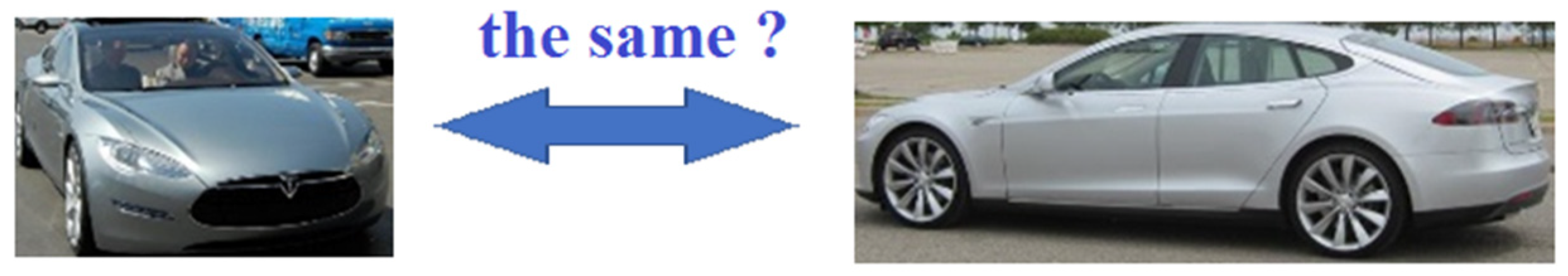A typical solution to such a task is to extract standard image features or descriptions (embedding vectors) generated by deep neural networks, and to classify them or to apply a hand-crafted decision by using vector–distance metrics (i.e., the Euclidean distance in vector space) [1,2]. The same image similarity problem becomes more difficult if the image content is a 3D object and the compared images present it from different viewpoints (Figure 1).

Direct comparison or classification of entire images (i.e., a front-to-end approach) by deep neural networks is a recent approach to image analysis [3,4,5,6] that has produced outstanding results. However, consider the problem of defining the “similarity” of two image sets and combine it with the problem of identifying the same “semantic” content, i.e., the same 3D object visible from different viewpoints. This complex problem appears in various real-world business scenarios, i.e., fraud detection, visual navigation, or product search. It is also useful in visual search or data duplication avoidance—for example, in a car insurance application process. A customer would have to take a set of photos of the car in order to for the insurance policy to start, and after an insurance event happens, the customer would have to take another set of photos of the same car. An automatic image set comparison system can improve the quality and speed of the claim handling process. The growing demand for visual similarity solutions is clear and comes from companies which seek effective answers for the aforementioned business problems. In recent years, some significant papers have been published about this topic. The first one mentioned here gives a review of a few methods developed for finding similar images in datasets [7]. Another important paper proposes a deep learning technique for the image similarity task called “DeepRanking” [8].

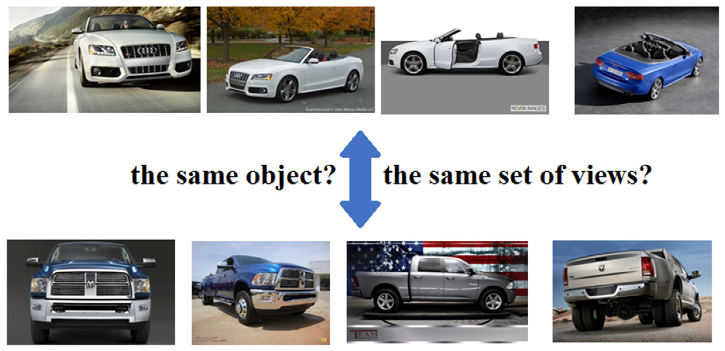
In this paper, we propose a solution to the image set comparison problem (Figure 2). This problem is analyzed in Section 2, while the proposed solution is described in Section 3. Our approach uses both image (more exactly: foreground object) classification and object-pair similarity evaluation procedures, and places them in a general-purpose framework system for image-set comparison. The solution requires not only the use of some category-level similarity, but also an instance-to-instance metric. Thus, the similarity score combines the evaluation of the visual content of image pairs with the comparison of image features computed from object ROIs (region of interest; the regions in the image which provide the needed information). We expect that the proposed solution might be deployed for comparisons of sets of images showing cars, cats, buildings, etc. An earlier developed base solution to the same problem is referred to in Section 4. The experimental verification of our approach is summarized in Section 5. The presentation of limitations and conclusions as well as a final discussion complete this paper.

The main objective is to provide answers to questions such as “is my set of images presenting the same object from the same viewpoint as the other set of images”. The object is application-dependent. The exact recognition of views and objects in particular images is not the question—the ultimate challenge is how to define a similarity measure for sets of object-centered images. During the search for a solution to this problem, we discovered that this case is nearly identical to the evaluation of multi-channel blind signal separation results [9], where the objective is to specify whether the set of M signals extracted from N mixtures is properly representing a (potentially unknown) set of M source signals. Our BSS-based similarity score takes into account object instances. We assume that other data analysis streams can support this process by considering the consistency of object types and views in both compared sets.

The contribution can be summarized as follows:

• a fusion of several image processing and classification streams is proposed to solve the problem of set-to-set similarity evaluation;
• a BSS error index [9]-based permutation-independent similarity score is proposed;
• the advantage of using a DeepRanking network [8], with its triplet loss function for image feature extraction and image-pair similarity, is confirmed in comparison with classic SIFT features [10];
• a quality improvement of a previous baseline approach is shown.

2. Problem and Related Work

2.1. Assumptions

Let us make some assumptions to constrain the general problem of image set comparison. First, we constrain the kind of 3D objects we would like to identify and compare. Here we shall distinguish the “image type” from “object type or category” and from the “context”. The question, “are the images of the same type?”, asks whether the object views are the same, i.e., a “front view” and a “side view” are examples of image types. The question, “are the visual objects of the same type?”, is related to single foreground objects detected in the image and classified according to our “context” (application domain). Object “categories” are generalizations of some types having the same basic properties.

Examples of object types in the category of “cars” can be: “vans”, “sedans”, “trucks”, and “lorries”. Examples of an application domain (context) are: cars for fraud detection for insurance companies or buildings and other urban infrastructure for visual navigation. The context can refer to single object categories (e.g., cars) or many object categories that can appear in the same image (e.g., “a car next to the tree” or “a car on the bridge”). In this work, we focus on the context of single cars present in an image.

2.2. Related Work

The primary problem of matching two image sets can be divided into subproblems such as:

• semantic segmentation (detection of the foreground object’s ROI),
• feature extraction,
• image-to-image similarity evaluation, and
• image set-to-image set similarity evaluation.

The literature doesn’t provide a complete solution to this problem, but we can find several papers related to these subproblems. The “DeepRanking” approach [8] is a comprehensive solution based on deep learning (DL) technology that provides both feature extraction and similarity evaluation of two images. We shall describe it in-detail in Section 4. The alternatives for the DL-based features can be hand-crafted keypoint descriptors, such as SIFT, speeded-up robust features (SURF), or “oriented features from accelerated segment test (FAST) and rotated binary robust independent elementary features (BRIEF)” (ORB) [10]. Several methods of this kind are compared in [11], paying attention to their performance for distorted images. Nowadays, computationally efficient binary keypoint descriptors dominate in real-time image analysis applications [12].

The next subproblem, how to measure a distance between images (or feature vectors), can be solved by the use of obvious metrics such as Euclidean, Manhattan, or Cosine distance or another, more specific one, such as the Hausdorff metric [1].

The evaluation of two image sets reminded us of the evaluation of blind source separation (BSS) algorithms as applied to the image sources [9]. There we faced a similar problem—every estimated output must have been uniquely assigned to a single source and, in an ideal case, should not contain any cross-correlation with other sources. We proposed an error index for both sets (separated outputs and reference sources) which handles the possible differences in permutation (ordering of images in a set) and amplitude scales, and is normalized by the number of set items.

Thus, our approach applies the DeepRanking-based DL stream of image pair comparison, the SIFT descriptors as ROI features, and the Euclidean distance in a conventional stream for image-to-image similarity evaluation. We also adapted the error index from BSS research to estimate the image sets dissimilarity score.

The architecture of multi-stream fusion of data analysis streams that covers all of the aforementioned subproblems into one final decision was chosen. The idea of such architecture was previously proposed in [13]. Different works [14,15,16] deal with multi-view image fusion to improve the results of single-view image analysis. The problems solved in these papers are different from our problem, yet the idea of using different views to obtain better results is close to our objective.

An overview of related papers, in accordance with a methodology to literature survey and evaluation developed in [17,18,19], is shown in

Table 1. An overview of related papers. X means “covered”. Citation count source is Google Scholar (last updated: 15 June 2021). Column explanation: I-2-I, set comparison based on comparison of image-to-image distance with Euclidean distance; DR, DeepRanking as a feature extraction method; SIFT, SIFT as a feature extraction method; BSS, a blind signal separation error index as a measure of the distance between two image sets; Car Model, a stream for car model classification.

Reference No	Year	Citations	No of References	Image			Feature		Distance Measures	Multi Stream Analysis	Image Set Comparison
				Classification	Comparison	Segmentation	Extraction	Comparison			I-2-I	DR	SIFT	BSS	Car Model
[1]	1999	167	23		X			X	X
[2]	2017	6	17		X
[3]	2013	1308	37	X
[4]	2013	38	23			X
[5]	2016	13861	23	X
[6]	2017	12098	35			X
[7]	2018	10	33		X			X	X
[8]	2014	1054	25	X	X		X	X
[9]	1997	9	14					X	X
[10]	2011	8238	30				X
[11]	2017	286	16				X	X
[12]	2014	47	8				X
[13]	2018	27	40							X
[14]	2007	202	33							X
[15]	2020	6	34							X
[16]	2019	45	46							X
[20]	2014	16326	51			X	X
[21]	2016	80936	49	X			X
[22]	2015	7939	23	X	X			X
[23]	2007	49	39					X		X
[24]	2021	-	11	X	X	X	X	X	X	X	X	X
Our	2021	-	25	X	X	X	X	X	X	X		X	X	X	X

.

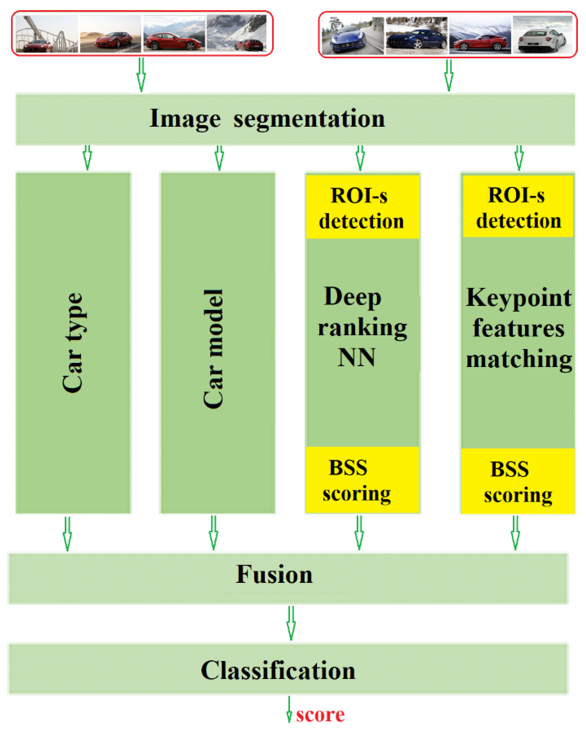
3. Solution

3.1. Structure

Our solution to image set similarity estimation is not limited by the number of images, and will be appropriate even for a single image pair. The core of this solution consists of four image processing streams for image-pair comparison (Figure 3):

• the classification of the foreground object type,
• the classification and the foreground object view,
• image-pair similarity based on semantic image segmentation (the DL stream), and
• feature-based image pair similarity (classic technique stream).

After accumulating similarity scores obtained for all image-pairs from the two analyzed image sets, the individual results are fused and further classified to obtain a final likelihood as to whether both sets contain the same object. The approach performs a multi-score “late fusion” (one possible approach to fuse multi-modal data, e.g., [14,15]), where the following scores are fused:

• The same-object (car)-type score (class likelihoods),
• The same-object (car)-model and -viewpoint score (class likelihoods),
• BSS error index (dissimilarity) based on all ROI image-to-image comparisons, and
• BSS error index based on the ROI-features comparison for all image pairs.

3.2. Image Segmentation

The input image sets always have the same number of images (otherwise both sets can immediately be declared as invalid). The Stanford Cars dataset [25] was used in experiments. It is a well-recognized car dataset providing model labels (annotation) and is cited in many research papers. It is freely available to the public and the attached annotation reduces the effort needed for training data preparation. The order of the images is not relevant (the solution must be invariant with respect to index permutation). We assume that each set has images of four views: the front, side, front-side and back-side view. Although in general our approach is view-independent—the user can decide to include any other sets of views—in our opinion, and for the given dataset, these views are the best selection. Our dataset does not have a good representative of back view images—this is the reason why we do not consider such a view. Every image is labeled by one of 4 views, 9 car types, and 197 car models. A class label “other” is also given to images which do not match any basic class.

Image segmentation follows the semantic segmentation approach based on a Mask-RCNN model [6]. To train the Mask-RCNN model, we used the COCO dataset (2017 version) [20]. COCO contains 81 categories of objects sufficient for training and testing the entire model. Semantic segmentation removes unnecessary parts of images and only keeps the parts that are consistent with the created model (application context). In particular, we focus on “Car” and “Truck” categories from the COCO dataset. The Mask-RCNN implementation uses a ResNet 101 [21] neural network architecture as the backbone.

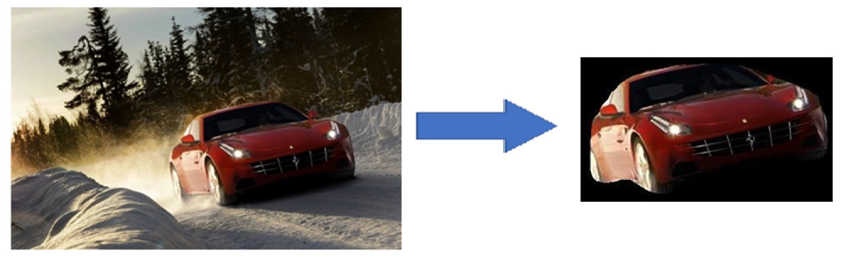
In Figure 4, an example of car mask detection results from two steps:

• the rectangular boundary box for car region extraction comes from the annotations given in the Stanford Car dataset, and
• the Mask RCNN generates the proper envelope of the car image region within the boundary box (from previous point).

3.3. Detection of ROIs

The ROIs detection step is the initial step of two alternative streams for set similarity scoring, based on deep neural networks or on classic key-point descriptors. We use the Selective Search [4] algorithm to find ROIs in images. Selective Search uses color, texture, size, and shape measures to characterize image regions and iteratively to perform hierarchical region grouping into ROIs. The list of obtained ROIs is ordered by area. We prefer to skip the one with the biggest size and to select the next five (2nd–6th) for further analysis. We chose this selection to avoid the whole car ROI and to concentrate on a fixed number of meaningful ROIs. To obtain ROI similarity scores, their feature vectors are obtained by two alternative methods: DeepRanking and the SIFT-descriptor.

3.4. DeepRanking Neural Network

Image-to-image comparison is a DL solution applied to foreground object ROIs detected in images. We measure the Euclidean distance between two embeddings produced by the CNN from the DeepRanking [8] approach. “FaceNet” was introduced in [22] and proposed the triplet loss function as a learning criterion. The triplet loss minimizes the distance between the anchor (query image) and the positive example image and maximizes the distance between the anchor and the negative example image. DeepRanking applies this triplet loss idea to learn an image-to-image similarity model. The triplet loss implementation in DeepRanking is as follows [8]:

$$\begin{array}{c}\min {\displaystyle \sum }_i{\epsilon }_i+\lambda {\Vert \mathit{W}\Vert }_2^2 s.t.: \max \left\{0,g+D\left(f\left(p_i\right),f\left(p_i^{+}\right)\right)-D\left(f\left(p_i\right),f\left(p_i^{-}\right)\right)\right\}\\ <{\epsilon }_i{\forall }_{p_i,p_i^{+},p_i^{-}};r\left(p_i,p_i^{+}\right)>r\left(p_i,p_i^{-}\right)\end{array}$$

(1)

where r is the image-pair similarity score. This score is responsible for ensuring that the positive image is more similar to the “average” one than the negative image. In our solution, we take positive images from the given class of model-view and negative images from another class of model-view. DeepRanking metric D is the Euclidean distance between two feature vectors. λ is a regularization parameter that controls the margin of the learned ranker to improve its generalization [8]. The g is a gap parameter that regularizes the gap between the distance of the two image pairs: (p_i, p_i⁺) and (p_i, p_i⁻). Function f(p) is the image embedding function. W is the parameters of the embedding function. It is considered to be one of the best neural network architectures for image matching (based on published results). Hence, we selected DeepRanking to obtain image-pair similarity scores.

3.5. Key-Point Feature Matching

In addition to DeepRanking, we use an alternative processing stream to obtain image pair similarity. Hand-crafted features (keypoints and their local descriptors) are extracted from the images. We apply the standard SIFT approach. Other schemes which are computationally more efficient and of similar quality such as SURF or ORB could also be used [10,11]. According to [11], SIFT gives the best image matching in most of the tested cases. In real-time applications, binary descriptors would be preferred [12].

3.6. BSS Scoring for Image Sets

Assume that similarity scores p_{i, j} are provided for every image pair (i, j), I = 1, 2, …, n and j = 1, 2, …, m. They are collected in a similarity matrix P = [p_ij], where p_ij = similarity (Ii, Ij). The error index (or dissimilarity score) for two image sets is defined as [9]:

$$EI\left(P\right)=\frac{1}{m}\left({\displaystyle \sum }_i{\displaystyle \sum }_j\left|{\tilde{p}}_{ij}\right|-n\right)+\frac{1}{n}\left({\displaystyle \sum }_j{\displaystyle \sum }_i\left|{\overline{p}}_{ij}\right|-m\right)$$

(2)

Two normalized versions of the matrix P are computed. In the first case, in every row of matrix P the maximum entry is found and all entries in a given row are divided by this maximum value:

• every row i of P is scaled: $\tilde{P}=Norm\left(P\right), such that {\forall }_i\left(ma{x}_j\left({\tilde{a}}_{ij}\right)=1\right)$

In the second case, the maxima are found independently in every column of P and the entries in every column are divided by their corresponding maximum value:

• every column j is scaled: $\tilde{P}=NormCol\left(P\right), such that {\forall }_j\left(ma{x}_i\left({\tilde{a}}_{ij}\right)=1\right)$.

Therefore, in an ideal case of two set matching, the first normalized matrix will have in every row only one nonzero entry equal to 1, while the second matrix will have a single entry 1 and all other entries in every column a 0. By subtracting from the sum of all row- or column-normalized elements the number of columns and rows, appropriately, the nonzero result will represent an average distance score between two images, while the one-valued entries will verify whether the checked set contains a single car model and all the required different views.

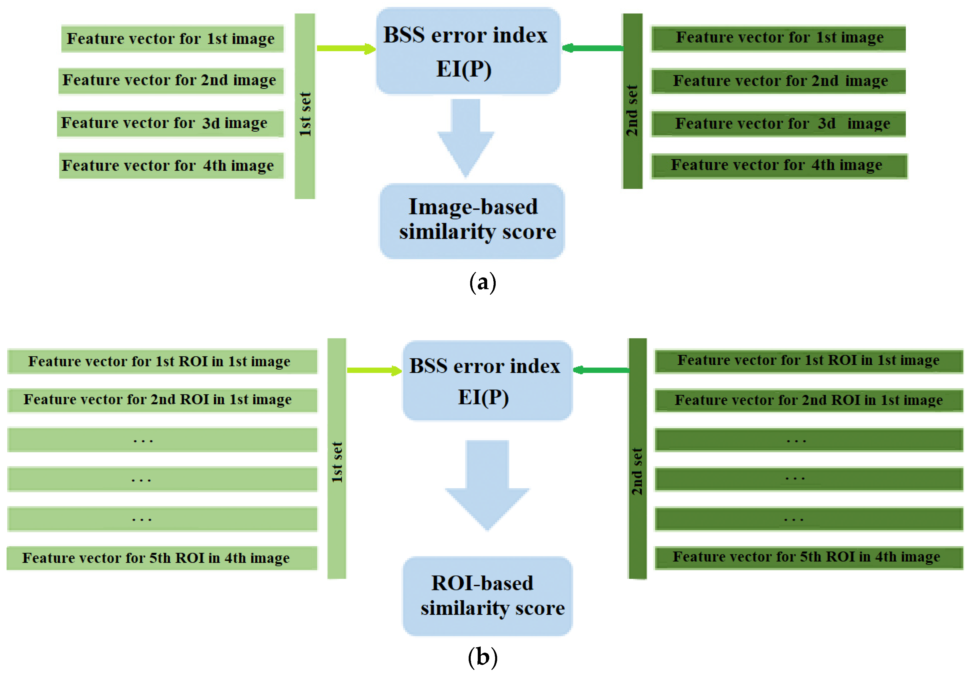
The BSS-based similarity score for two sets is obtained in two different modes—the image-to-image comparison mode and the ROI-to-ROI comparison mode (Figure 5). In the first case, a feature vector (DeepRanking embeddings or SIFT descriptors) is calculated for every (masked) image in every set. The similarity matrix P is of size 4 × 4, where every entry represents the similarity score for the features of a pair of images (Figure 5a). In the second mode, every image from a set of four images is represented by five ROIs and their feature vectors (DeepRanking embeddings or SIFT descriptors) are given. Thus, we calculate the BSS error index (EI(P)) for a 20 × 20 similarity matrix P, where the first set ROIs play the role of the “BSS sources”, while the second set ROIs are the estimated “separated signals” (Figure 5b).

3.7. Car Model Classifier

Car model classifier is needed to boost the accuracy of the image set comparison score. We have a closed list of the models (classes) available for the problem. The classifier is defined as a pretrained neural network based on the Inception V3 [5] architecture with 197 classes (196 cars and one “other” class).

$$\left[\begin{array}{c}c{m}_{11}\\ .\\ \begin{array}{c}.\\ c{m}_{41}\end{array}\end{array}\begin{array}{c}.\\ \\ \begin{array}{c} \\ .\end{array}\end{array}\begin{array}{c}.\\ \\ \begin{array}{c} \\ .\end{array}\end{array}\begin{array}{c} \\ \\ \begin{array}{c} \\ \end{array}\end{array}\begin{array}{c} \\ \\ \begin{array}{c}c{m}_{im}\\ \end{array}\end{array}\begin{array}{c}.\\ \\ \begin{array}{c} \\ .\end{array}\end{array}\begin{array}{c}.\\ \\ \begin{array}{c} \\ .\end{array}\end{array}\begin{array}{c}c{m}_{1 197}\\ .\\ \begin{array}{c}.\\ c{m}_{4197}\end{array}\end{array}\right]$$

(3)

For each image, I (I = 1, …, 4), its similarity scores with respect to the 197 models are obtained. The highest scored model is selected as an image vote. The class with the majority of votes given by the images in a set is selected as the set’s winner [23].

$$CM=\left(m_1,m_2,m_3,m_4\right),\mathrm{where}{m}_i=\underset{j}{\mathrm{argmax}}c{m}_{ij}$$

(4)

3.8. Car Type Classifier

The purpose of the car type classifier is to determine the general type of the car presented in all images of a set. There are eight types distinguished: Van, Sedan, Coupe, SUV, Cabriolet, Hatchback, Combi, and Pickup, with four views for each type, and the “other” class for non-recognized types. This classifier is also based on the InceptionV3 [5] deep neural network. For each image in a set, the highest scored type is selected as the image vote. The class with the majority of votes given by the images in a set is selected as the set’s winner [23].

$$\left[\begin{array}{c}c{t}_{11}\\ .\\ \begin{array}{c}.\\ c{t}_{41}\end{array}\end{array}\begin{array}{c}.\\ \\ \begin{array}{c} \\ .\end{array}\end{array}\begin{array}{c}.\\ \\ \begin{array}{c} \\ .\end{array}\end{array}\begin{array}{c}.\\ \\ \begin{array}{c} \\ .\end{array}\end{array}\begin{array}{c} \\ \\ \begin{array}{c}c{t}_{it}\\ \end{array}\end{array}\begin{array}{c}.\\ \\ \begin{array}{c} \\ .\end{array}\end{array}\begin{array}{c}.\\ \\ \begin{array}{c} \\ .\end{array}\end{array}\begin{array}{c}c{t}_{141}\\ .\\ \begin{array}{c}.\\ c{t}_{441}\end{array}\end{array}\right]$$

(5)

$$CT=\left(f{t}_1,f{t}_2,f{t}_3,f{t}_4\right),\mathrm{where}f{t}_i=\underset{ j}{\mathrm{type}(\mathrm{argmax}}c{t}_{ij})$$

(6)

Remark: type () gets the type index from the view-type class identifier.

3.9. Fusion

Fusion is the layer where results from all streams are combined into one vector v of all available scores. This vector is classified in the final classification step:

$$v=\left(\begin{array}{ccc}C{T}_1,C{T}_2,& C{M}_1,C{M}_2,& \begin{array}{cc}i-to-i,& ROI-to-ROI\end{array}\end{array}\right)$$

(7)

where:

• CT_i is the indicator vector for car type for the i-th set,
• CM_i is the car model indicator vector for the i-th set,
• i-to-i is the value of the two-set similarity score based on the BSS error index obtained in image mode, and
• ROI-to-ROI is the value of the two-set similarity score based on the BSS error index obtained in ROI mode.

3.10. Final Classification

Final classification gives the estimated similarity score of both image sets provided at the system’s input. This step is implemented as a feedforward neural network with four fully connected layers (see a detail description of layers in

Table 2. Architecture of the final classifier in our solution.

Layer Number	Type of the Layer	Output Size
1	Dense	6
2	Batch normalization	6
3	Dense	18
4	Batch normalization	18
5	Dense	18
6	Batch normalization	18
7	Dense	2

). The fused vector (Equation (7)) is a rather short one. Thus, the neural network can have a simple architecture. The final score is in the interval 0–1, where 0 represents “different” objects, while 1 means the same object exists in both sets.

4. The Base Solution

In the experiments, we are going to compare the current approach with an earlier developed base solution [24]. Several modifications have been made—they are summarized as follows:

• Now we calculate the BSS-based similarity score to resolve the unknown permutation of views in two sets.
• The base system has no car model stream.
• Additionally, to the “image-to-image-mode”, given in the baseline, in the presented approach the similarity score in the “ROI-to-ROI” mode is also computed.
• The final classification network has been simplified. Compare the current classifier network (Table 2) with such a network in the base solution (

  Table 3. Architecture of the final classifier for the base solution.

  Layer Number	Type of the Layer	Output Size
  1	Dense	64
  2	Batch Normalization	64
  3	Dense	128
  4	Batch Normalization	128
  5	Dense	196
  6	Batch Normalization	196
  7	Dense	128
  8	Batch Normalization	128
  9	Dense	2

  ).

Although the two new results are fused, due to the use of the explicit BSS score the fused vector is now of the same length as before (18 elements). It also turned out that the size of the final classification network can be much lower than in the baseline.

5. Results

For an experimental evaluation, the Stanford Cars dataset [25] was used. We fixed the number of images in every image set to four. The order of views in the set is not relevant. We assumed that each proper set has four views: front, side, front-side, and back-side. Obviously, the approach is view-independent and in other applications any other number of views can be set. This doesn’t mean that with different views we can get the same quality of results. The choice of a specific kind of view depends on the user’s decision and their experience. From a technical and methodological point of view, our solution is independent of the selection of object views. Our dataset has less accurate data of back view images, so we decided to skip this view. Hence, the dataset is labeled by 4 views, 9 car types, and 197 car models. Both types of object-related label contain the class other for images which are not matched with the basic labels.

We conducted several experiments with this dataset and different settings of the system, and produced much improved results compared with the earlier base solution. The assumptions for the experiments are described in

Table 4. Average accuracy of the similarity of two image sets.

Model	Accuracy
Base solution (DeepRanking + Euclidean distance) [24]	50.2%
Proposed with DeepRanking and BSS score, without car model stream	62.1%
Proposed with DeepRanking and BSS score and car model stream	67.7%
Proposed with SIFT and BSS score, without car model stream	61.6%
Proposed with SIFT and BSS score and car model stream	64.4%

. With the same dataset we used, alternatively, DeepRanking- or SIFT-based features, and turned on or off an additional stream for car model classification. The dataset was split into learning (70%) and test parts (30%), and every experiment was repeated 10 times with different dataset splits. In Table 4, the average accuracy rates of different configurations of the proposed solution and the base solution are presented. By “accuracy”, we mean the “genuine acceptance rate” (GAR) of a recognition system when “false acceptance rate” (FAR) is kept at 3%. The summarized accuracy of set-similarity recognition was increased from 50.2%, for the best baseline setting, to 67.7% for the best option of proposed approach. The best architecture appeared to include the (additional) car model classification stream and the DeepRanking net for feature extraction (instead of the SIFT descriptor).

As we can clearly see in Table 4, the use of an explicit BSS error index as a measure of permutation-independent distance between two image sets and the additional car model classification stream allow for a significant improvement in the set similarity classification accuracy. For image feature extraction, it is more advantageous to use the DeepRanking approach than the classic SIFT descriptor.

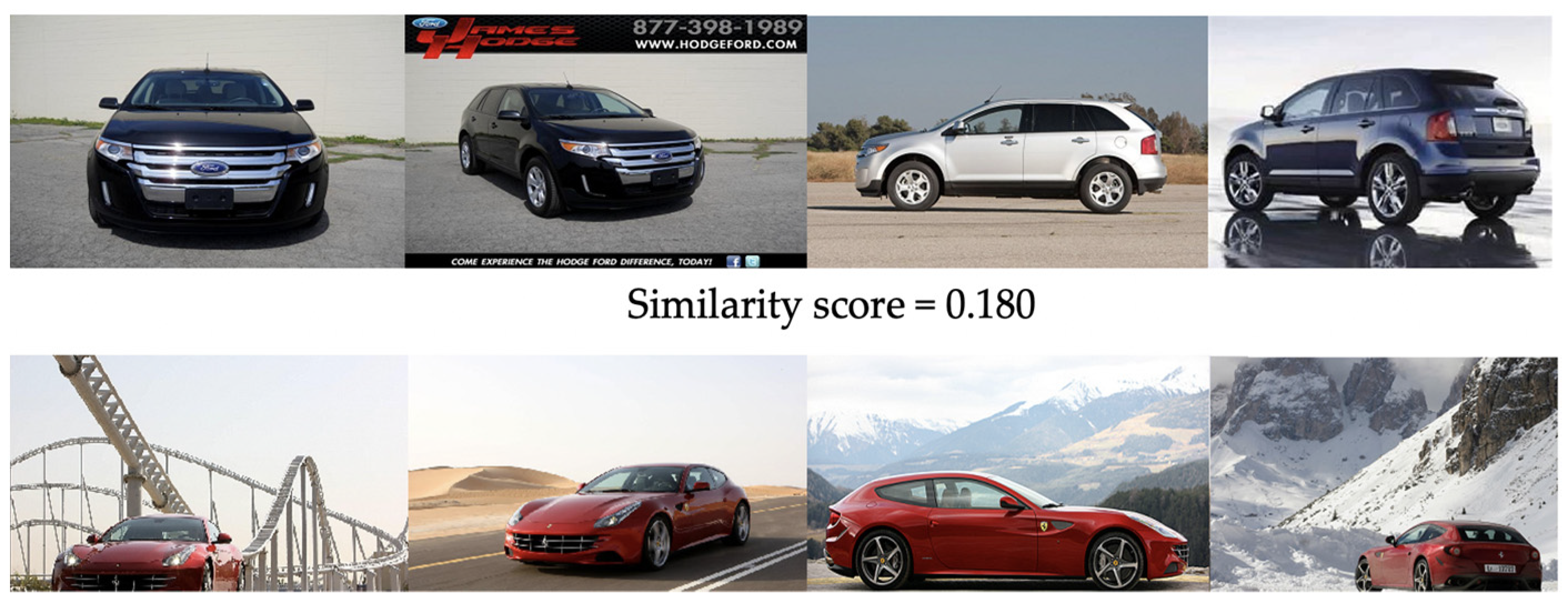
At first glance, the accuracy value of 67.7% seems to be a relatively worse result. However, the considered problem is rather hard to solve. Let us illustrate the results in more detail, by considering three different set-versus-set situations (

Table 5. Average final set-similarity scores for different situations.

Case	Base Approach [24]	Proposed	Should Be
Same car model and same view	0.708	0.821	1.0
Same car model but different views	0.531	0.597	~0.5
Different car model	0.208	0.180	0.0

):

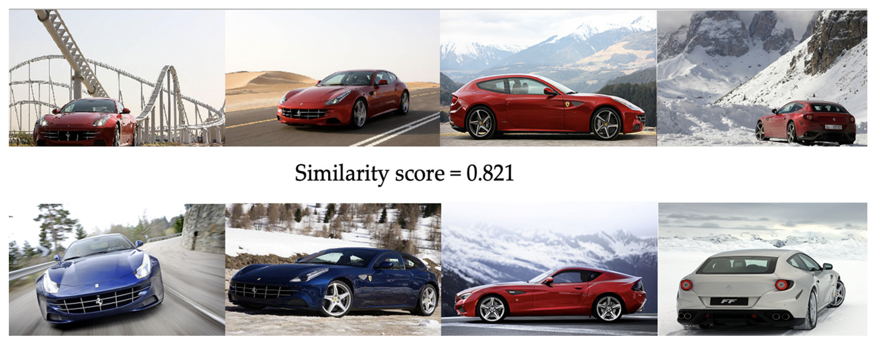
• the same car model and the same views in both sets (Figure 6),
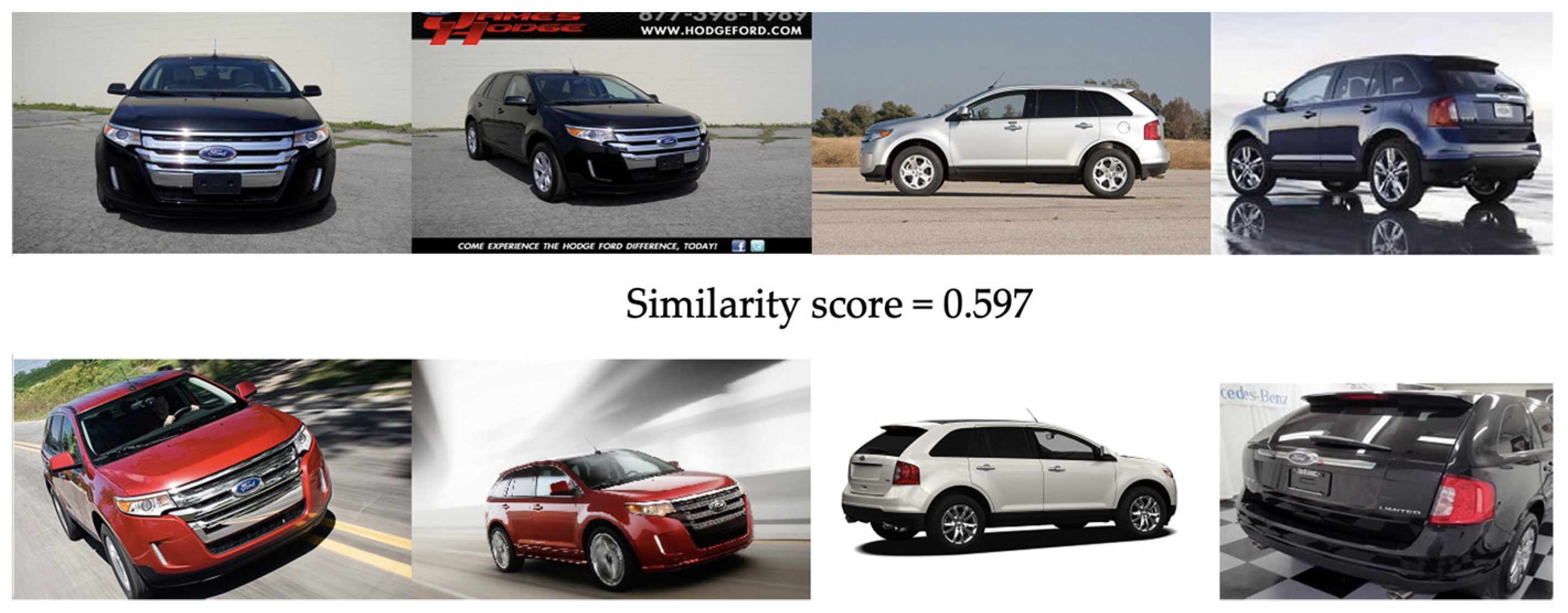
• the same car model but inconsistent views (Figure 7), and
• different car models (Figure 8).

In comparison with the base solution, the discrimination ability of the similarity score is much improved—the discrepancy between different- and same-set average score is raised from 0.500 (=0.708–0.208) to 0.641 (=0.821–0.180). However, the score is still sensitive to even small changes of the viewpoint direction, even when only one image-pair in the set is affected by such a situation. An image-pair similarity score of around 0.5 may result from obviously different views or from a visible change of the viewpoint direction, but within the same view type (see Figure 9). Although every individual score only partly contributes to the final set-similarity score, one low score alone affects the overall set-related score. For the final decision, we applied a conservative threshold that corresponds to a false acceptance rate of 3% (in every configuration). The focus on false acceptance avoidance leads to a relatively low accuracy ratio (67.7%). The overall score is obviously dependent on the quality of individual data analysis streams. Let us observe the average accuracy (GAR at 3% FAR) of some individual streams and the image segmentation step obtained in the experiments:

• accuracy of the single-image car type classification stream was 75.1%,
• single-image car model classification accuracy was 66.3%, and
• accuracy of the semantic segmentation (a subjective evaluation of the proper detection of the car mask region) was 89.7%.

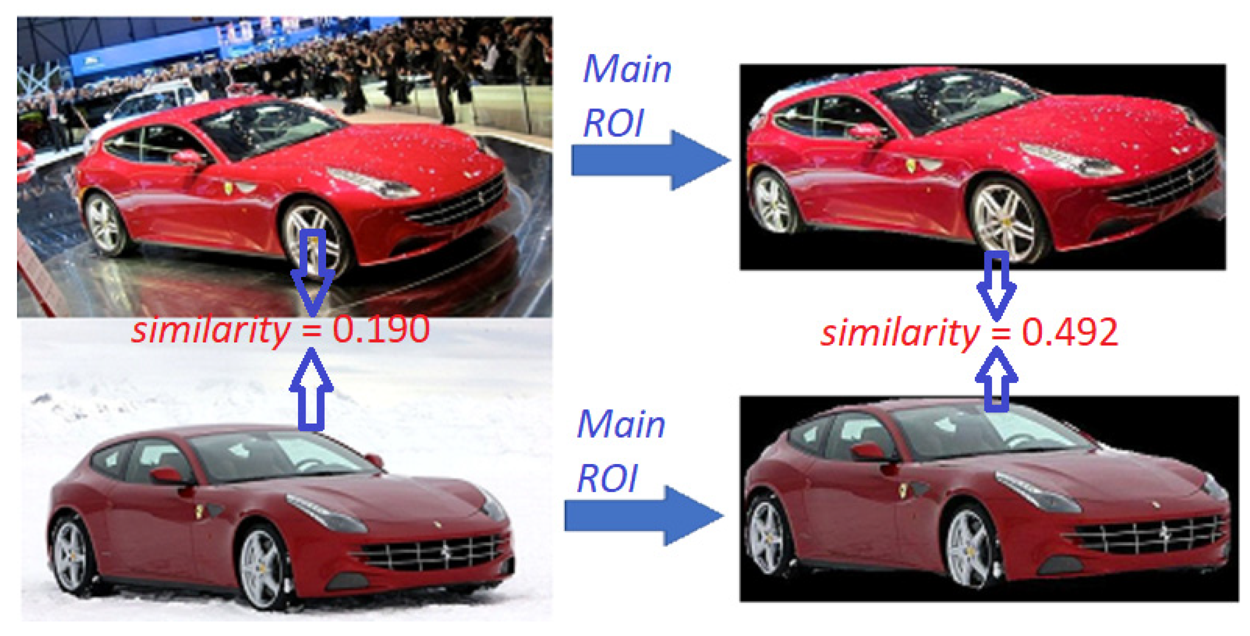
It is clearly visible that a proper detection of the object’s ROI in the image allows for the improvement of the classification accuracy of the entire approach. Let us illustrate this fact with an example. In Figure 9, two different cars of the same type and model are compared two times—by matching entire images (the left pair of images) and by matching the previously detected object ROIs (the right pair of images). We expect that the proper similarity score for the same view of the same car model should be rather high (>0.5). For the set of images on the left, we got a low similarity score of 0.190 (the same car model under a slightly different view but with a very different background), while for the ROI image pair on the right side the score was 0.492 (where the background was eliminated in ROI masked images).

6. Limitations

Our approach and proposed solution have several limitations. The first being that our approach cannot be applied to any image content; the proposed solution is valid only for images with a single foreground object. The second limitation is that we are matching object views, but we do not make view registration (i.e., view normalization) by transforming image content. If an image pair shares the same type of object view but the viewpoints differ too much, the similarity score may be lower than needed. Two other limitations are of technical nature, as we require the same granularity of labels in the dataset and require the same number of images in both sets. All of these limitations can be considered in future research and some of them will be relatively easily addressed.

7. Conclusions

An approach to image-set similarity evaluation was proposed based on the fusion of several image processing and classification streams. The achieved experimental results confirmed that the new solution’s steps, as proposed in this paper, give a visible improvement of the previous baseline approach. They include an additional car model classification stream and the use of an explicit BSS-based permutation-independent score of image sets. Once more, the advantage of using a DeepRanking network with its triplet loss function for image feature extraction was confirmed. The evaluation of image-pair similarity results obtained by the DeepRanking stream has demonstrated its strengths over a classic stream based on SIFT features. Another conclusion from this work is the importance of using application-dependent classification streams (e.g., the car type and car model-and-view information), representing semantic content information and not solely application-independent streams for image similarity evaluation. The car model classification stream has improved our results by another few points.

8. Discussion

We have shown that a multi-stream fusion of application-independent and semantic streams is a prospective approach to image-set similarity evaluation. Our approach gives strong advice on the design of a generalized framework. The design of application-independent streams (e.g., image similarity scoring) should preferably use machine learning-based features instead of hand-crafted features, however, the use of smart distance metrics (e.g., BSS error index) is extremely important. A correct selection of semantic processing streams is also strongly recommended. In the context of using machine learning methodology, the required semantic data sets are much easier to obtain and label than the data needed for universal model creation.

In future research, we would like to generalize the approach by adopting it to other object categories. Explainable AI (XAI) techniques are also of interest to explain the contribution of particular processing streams and steps to the overall result. XAI techniques allow us to answer an important set of questions: not only whether something is similar, but also why it is similar. This would enable a further generalization of our approach, which could be applied not only in image set comparison, but in other pattern sets as well (e.g., text or multi-modal sets of sources).

References

- Gesù, V.; Starovoitov, V. Distance-based functions for image comparison. Pattern Recognit. Lett. 1999, 20, 207–214. [Google Scholar] [CrossRef]
- Gaillard, M.; Egyed-Zsigmond, E. Large scale reverse image search: A method comparison for almost identical image retrieval. In Proceedings of the INFORSID, Toulouse, France, 31 May 2017; p. 127. Available online: https://hal.archives-ouvertes.fr/hal-01591756 (accessed on 23 June 2021).
- Krause, J.; Stark, M.; Deng, J.; Fei-Fei, L. 3D Object Representations for fine-grained categorization. In Proceedings of the 2013 IEEE International Conference on Computer Vision Workshops, ICCVW 2013, Sydney, Australia, 1–8 December 2013; pp. 554–561. [Google Scholar] [CrossRef]
- Uijlings, J.R.R.; Van De Sande, K.E.A.; Gevers, T.; Smeulders, A.W.M. Selective search for object recognition. Int. J. Comput. Vis. 2013, 104, 154–171. [Google Scholar] [CrossRef]
- Szegedy, C.; Vanhoucke, V.; Ioffe, S.; Shlens, J.; Wojna, Z. Rethinking the inception architecture for computer vision. In Proceedings of the 2016 IEEE Conference on Computer Vision and Pattern Recognition (CVPR), Las Vegas, NV, USA, 27–30 June 2016; pp. 2818–2826. [Google Scholar] [CrossRef]
- He, K.; Gkioxari, G.; Dollar, P.; Girshick, R. Mask R-CNN. In Proceedings of the 2017 IEEE International Conference on Computer Vision (ICCV), Venice, Italy, 22–29 October 2017; pp. 2980–2988. [Google Scholar] [CrossRef]
- Kavitha, K.; Sandhya, B.; Thirumala, B. Evaluation of Distance measures for feature based image registration using AlexNet. Int. J. Adv. Comput. Sci. Appl. 2018, 9, 284–290. [Google Scholar] [CrossRef]
- Wang, J.; Song, Y.; Leung, T.; Rosenberg, C.; Wang, J.; Philbin, J.; Chen, B.; Wu, Y. Learning Fine-Grained Image Similarity with Deep Ranking. In Proceedings of the 2014 IEEE Conference on Computer Vision and Pattern Recognition (CVPR), Columbus, OH, USA, 23–28 June 214; pp. 1386–1393. [CrossRef]
- Kasprzak, W.; Cichocki, A.; Amari, S. Blind source separation with convolutive noise cancellation. Neural Comput. Appl. 1997, 6, 127–141. [Google Scholar] [CrossRef]
- Rublee, E.; Rabaud, V.; Konolige, K.; Bradski, G. ORB: An efficient alternative to SIFT or SURF. In Proceedings of the 2011 International Conference on Computer Vision, Barcelona, Spain, 6–13 November 2011; pp. 2564–2571. [Google Scholar] [CrossRef]
- Karami, E.; Prasad, S.; Shehata, M. Image matching using SIFT, SURF, BRIEF and ORB: Performance comparison for distorted images. arXiv 2017, arXiv:1710.02726. Available online: https://arxiv.org/abs/1710.02726 (accessed on 23 June 2021).
- Figat, J.; Kornuta, T.; Kasprzak, W. Performance Evaluation of Binary Descriptors of Local Features. In Proceedings of the International Conference on Computer Vision and Graphics, ICCVG 2014, Warsaw, Poland, 15–17 September 2014; Chmielewski, L.J., Kozera, R., Shin, B.S., Wojciechowski, K., Eds.; Springer: Cham, Switzerland, 2014; Volume 8671, pp. 187–194. [Google Scholar] [CrossRef]
- Zhao, P.; Liu, K.; Zou, H.; Zhen, X. Multi-stream convolutional neural network for sar automatic target recognition. Remote Sens. 2018, 10, 1473. [Google Scholar] [CrossRef]
- Swoger, J.; Verveer, P.; Greger, K.; Huisken, J.; Stelzer, E.H.K. Multi-view image fusion improves resolution in three-dimensional microscopy. Opt. Express 2007, 15, 8029–8042. [Google Scholar] [CrossRef] [PubMed]
- Fadadu, S.; Pandey, S.; Hegde, D.; Shi, Y.; Chou, F.C.; Djuric, N.; Vallespi-Gonzalez, C. Multi-view fusion of sensor data for improved perception and prediction in autonomous driving. arXiv 2020, arXiv:2008.11901. Available online: https://arxiv.org/abs/2008.11901 (accessed on 23 June 2021).
- Wei, W.; Dai, Q.; Wong, Y.; Hu, Y.; Kankanhalli, M.; Geng, W. Surface-Electromyography-based gesture recognition by multi-view deep learning. IEEE Trans. Biomed. Eng. 2019, 66, 2964–2973. [Google Scholar] [CrossRef] [PubMed]
- Shaukat, K.; Luo, S.; Varadharajan, V.; Hameed, I.A.; Xu, M. A survey on machine learning techniques for cyber security in the last decade. IEEE Access 2020, 8, 222310–222354. [Google Scholar] [CrossRef]
- Alam, T.M.; Shaukat, K.; Hameed, I.A.; Luo, S.; Sarwar, M.U.; Shabbir, S.; Li, J.; Khushi, M. An investigation of credit card default prediction in the imbalanced datasets. IEEE Access 2020, 8, 201173–201198. [Google Scholar] [CrossRef]
- Shaukat, K.; Luo, S.; Varadharajan, V.; Hameed, I.A.; Chen, S.; Liu, D.; Li, J. Performance comparison and current challenges of using machine learning techniques in cybersecurity. Energies 2020, 13, 2509. [Google Scholar] [CrossRef]
- Lin, T.; Maire, M.; Belongie, S.; Hays, J.; Perona, P.; Ramanan, D.; Dollár, P.; Zitnick, C.L. Microsoft COCO: Common objects in context. In Computer Vision – ECCV 2014. ECCV 2014. Lecture Notes in Computer Science; Fleet, D., Pajdla, T., Schiele, B., Tuytelaars, T., Eds.; Springer: Cham, Switzerland, 2014; Volume 8693, pp. 740–755. [Google Scholar] [CrossRef]
- He, K.; Zhang, X.; Ren, S.; Sun, J. Deep residual learning for image recognition. In Proceedings of the 2016 IEEE Conference on Computer Vision and Pattern Recognition (CVPR), Las Vegas, NV, USA, 27–30 June 2016; pp. 770–778. [Google Scholar]
- Schroff, F.; Kalenichenko, D.; Philbin, J. FaceNet: A unified embedding for face recognition and clustering. In Proceedings of the 2015 IEEE Conference on Computer Vision and Pattern Recognition (CVPR), Boston, MA, USA, 8–12 June 2015; pp. 815–823. [Google Scholar] [CrossRef]
- Goh, D.H.; Ang, R.P. An introduction to association rule mining: An application in counseling and help-seeking behavior of adolescents. Behav. Res. Methods 2007, 39, 259–266. [Google Scholar] [CrossRef][Green Version]
- Piwowarski, P.; Kasprzak, W. Multi-stream fusion in image sets comparison. In Automation 2021: Recent Achievements in Automation, Robotics and Measurement Techniques. AUTOMATION 2021. Advances in Intelligent Systems and Computing; Szewczyk, R., Zieliński, C., Kaliczyńska, M., Eds.; Springer: Cham, Switzerland, 2021; Volume 1390, pp. 230–240. [Google Scholar] [CrossRef]
- Krause, J. Stanford Cars Dataset. Available online: http://ai.stanford.edu/~jkrause/cars/car_dataset.html (accessed on 23 June 2021).