
Operational Resilience Metrics for Complex Inter-Dependent Electrical Networks

 , ,
, ,  ,
,  ,
,  and
and
Abstract
:1. Introduction
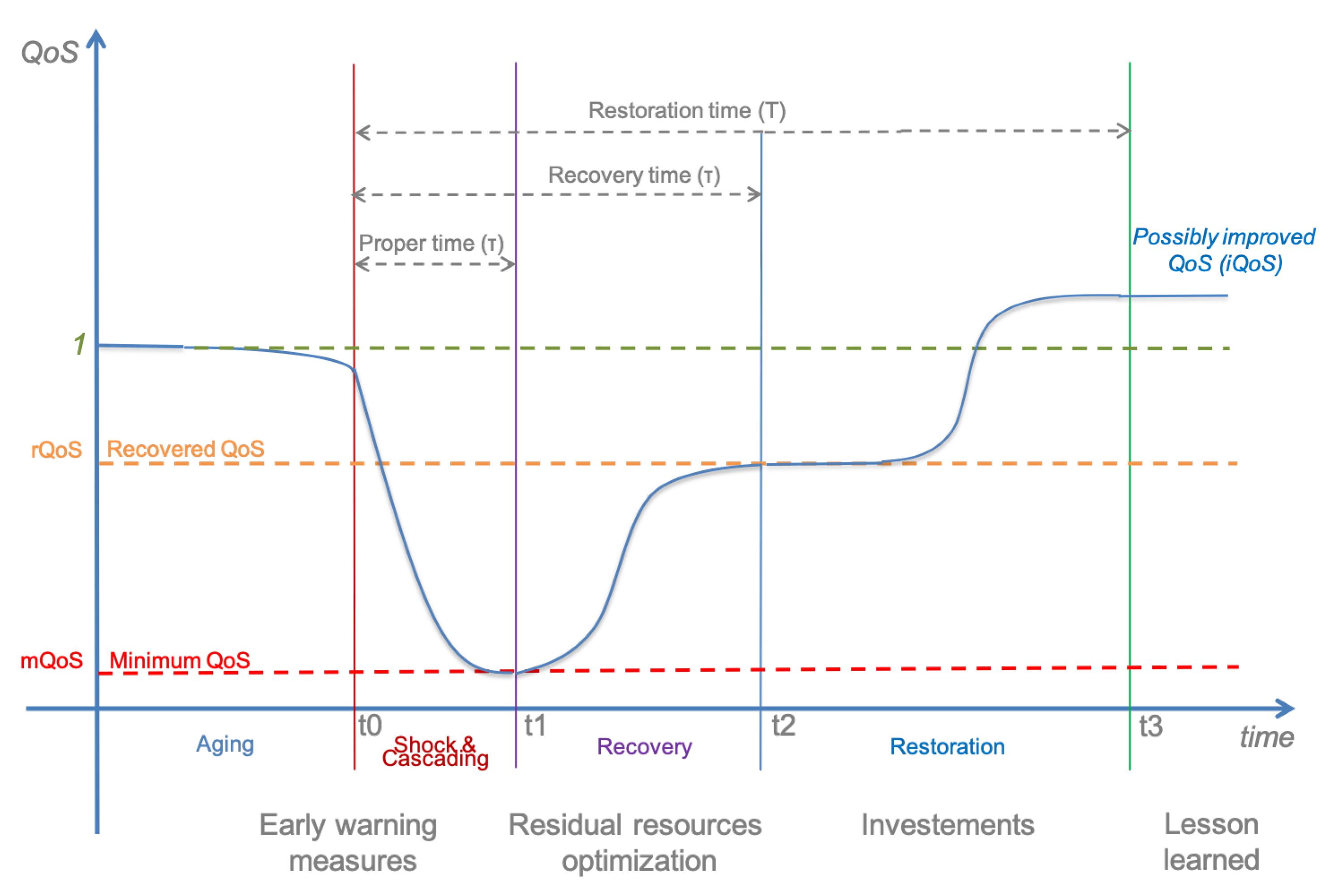
- Normal behavior and aging (). During this phase, in the absence of perturbations, the QoS of the system is optimal. The service is delivered thus producing the “wealth” of all users. Maintenance actions are required to maintain this optimal (or near-optimal) behavior. During this phase, events prediction and the set up of preparedness actions should be considered.
- Shock (). This phase follows a perturbation. From this point on, the QoS typically decays rapidly following an exponential behavior. The decay rate depends on the infrastructure and might vary from a few seconds to hours. In an EDN, for instance, protection devices and/or procedures require the disconnection or isolation of system components to avoid the spreading of the impact. The decay behavior of this phase could be affected by several factors: involvement of a large number of components, and possible negative feedbacks from interdependent networks [17]. Shock phase ends up at time corresponding to the time when CI operators starts acting on the network control and where: reaches the minimum.
- Recovery ( where: ). This phase starts when the activity of contingency management is implemented to recovery from the fault through automatic and manual interventions in order to increase the QoS. Success in the recovery phase, however, could be hindered, again, by negative feedback arising from the losses in other services; they could reduce the efficiency of recovery strategies (i.e., the absence of tele-control functionality, reduced by a severe electric outage, would force the use of longer manual restoration procedures). In general, this phase has the primary goal to start supplying services to critical users through the rapidly deployable contingency actions.
- Restoration ( where: ). This phase, which might extend on time scales larger than those of the previous phases, allows us to recover the full functionality of the network (i.e., the QoS before the perturbation, if possible). In principle, a wise and efficient restoration phase could also originate new properties of the network, which might produce a super-elastic behavior, i.e., allowing the system to gain a larger QoS with respect to that displayed before the crisis (i.e., a new network configuration could guarantee the service supply with lesser operational costs in term of electrical losses).
- EDN-robustness of main components. The robustness of the EDN components has to do with their ability to withstand stress while sustaining limited or no damage. The structural hardening or in any case structural suitability of the main power delivery components, such as individual substations, transmission lines and distribution feeders, is a common approach to decrease vulnerability, i.e., their propensity to sustain damage if stressed, and enhance electric power system robustness. The magnitude of the loss of functionality at the time of the shock, i.e., of Figure 2 mainly depends on the robustness of main EDN components;
- EDN topology. The topology of the network has a significant impact on its robustness and functionality. For the EDN, the term topology encompasses both the graph structure of the network and the position of the switches along the distribution lines. Both the properties have an impact in determining the overall resilient response of the network ([21] and references therein);
- Tele-controlled devices. A large fraction of CI elements along the distribution network is tele-controlled, i.e., their control could be remotely performed by using telecommunication systems. Among them, “automatic” CI elements allow for a rapid decoupling of the faulted branch from the rest of the line. The lower the number of such units, the weaker the remote controllability of the system and the longer the required restoration time;
- EDN-Telecommunication dependencies. The topology of the EDN-Telco interconnection, to discover how perturbation spreads on the different networks and which feedback should be expected;
- Efficiency of remote-controlled devices. This can be achieved by redundant connections to telecommunication networks or private (and more secure) proprietary, wired communication networks;
- Efficiency of restoration procedures. This can be achieved, for instance, by decreasing the time required to carry out the different restoration actions including tele-controlled and manual actions;
- Number of available technical crews. The amount of technical resources available on the field when manual interventions on CI elements are required can lower the time of the intervention.
2. Operational Resilience Metric for Electrical Distribution Networks
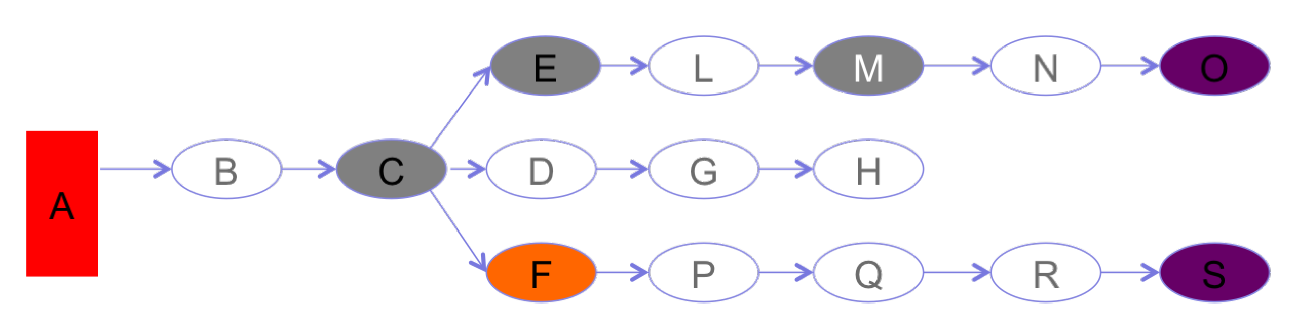
- vertex set with ;
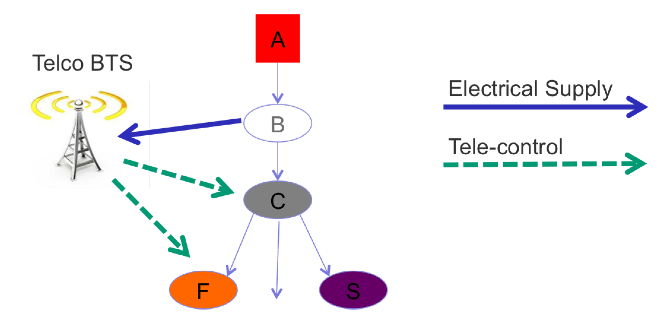
- represents an electric primary station (PS) containing high-to-medium tension transformers equipped with remote control functionality provided by a proprietary telecommunication network;
- represents an electric secondary station () containing medium-to-low tension transformers equipped with remote controlled switches (that depend on some BTS ;
- represents an electric secondary station () containing medium-to-low tension transformers equipped with automatic switches;
- represents an electric secondary station () containing medium-to-low tension transformers without remote control functionality;
- edge set where the generic represents the portion of an electrical line connecting the two electric stations and ;
- weight set associated to each vertex where: (i) on represents a physically intact and fully available station, (ii) disc represents a physically intact and functionally unavailable station and (iii) dam represents a physically damaged and functionally unavailable station;
- each is electrically supplied by a specific s.t. .
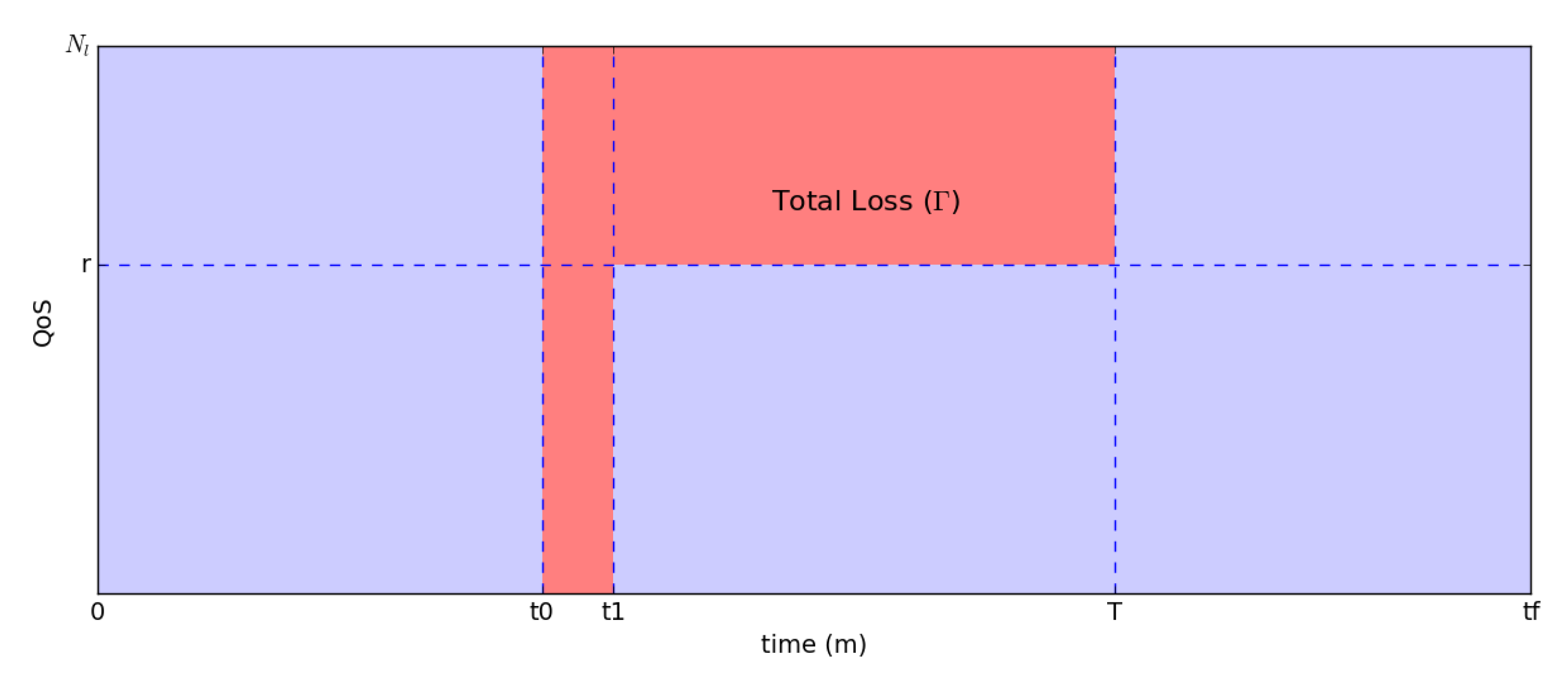
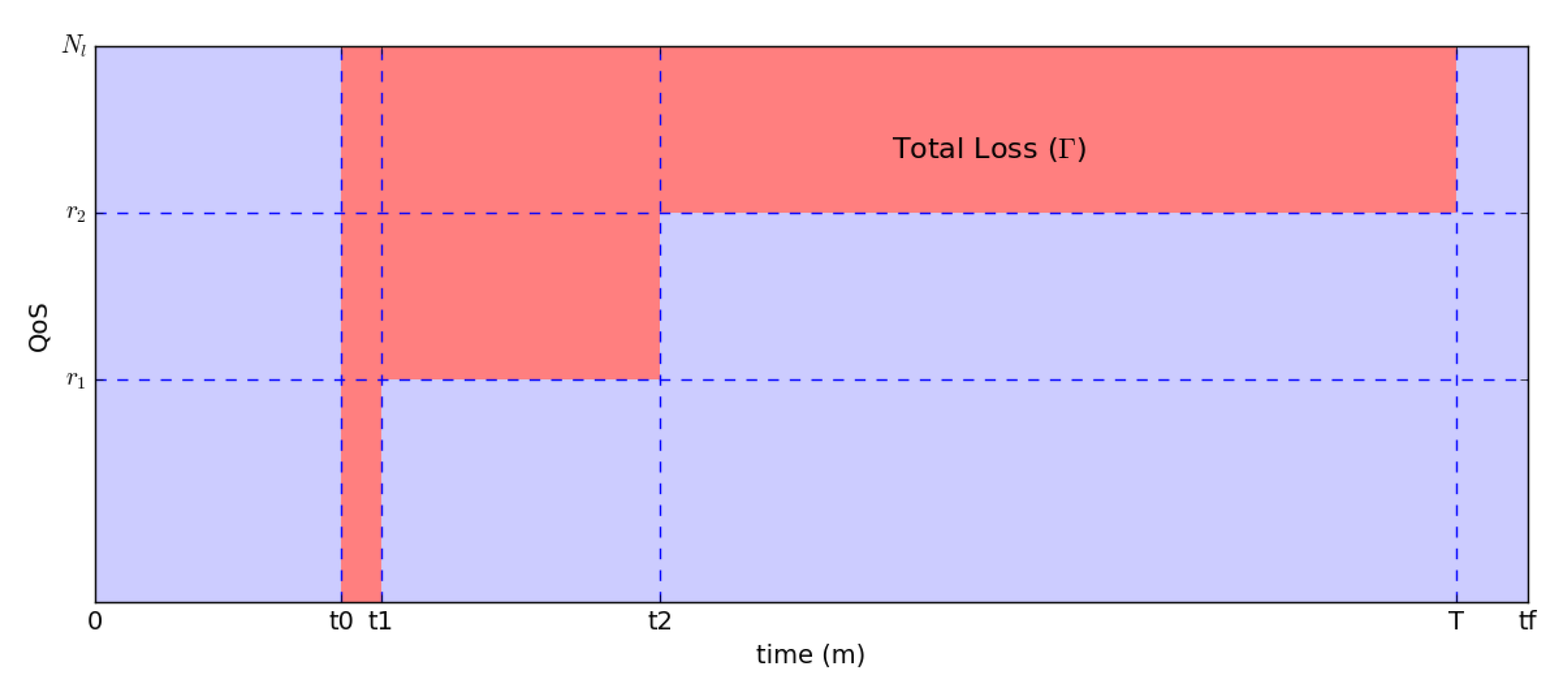
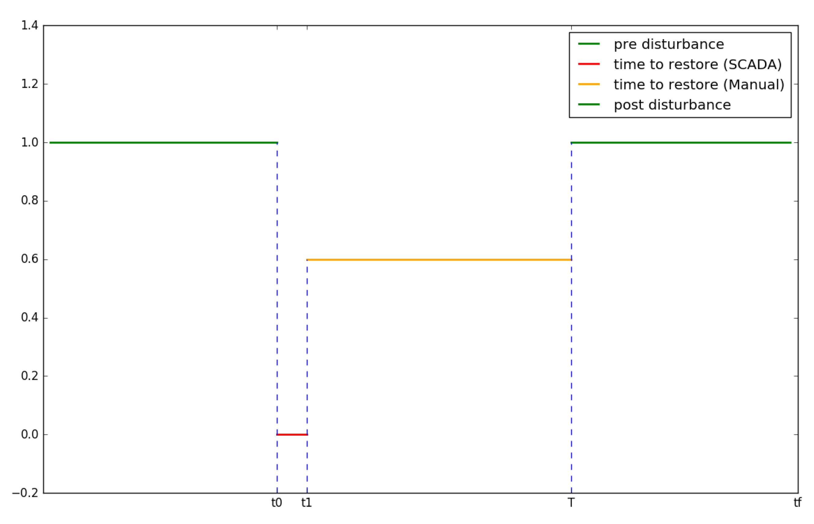
- . The QoS of the line reaches the maximum value if the line is not perturbed or when, after a perturbation, the line is completely restored within a time interval T (pre and post disturbance green lines of Figure 3).
- . The QoS for the line l reaches the minimum value at time when there exists at least one in the line l is in the dam state. For EDN medium-voltage lines the QoS almost instantly reaches the minimum value (i.e., the zero value) because of the opening of protection devices that disconnect all electrical SS in the interested line.
- for . The electrical utility operator using the SCADA system (if available) is able to restore the service in a number of substations of the line l. The time-to-restore by SCADA value is, in general, short. According to the electrical utility operator of the metropolitan area of Rome (Areti SpA) this value is approximately 3 min. The value r will depend on the number of substations that can be restored by remote actions. More of these substations are closer to the r value than they will be to M. Anyway, in general, there exist substations that cannot be restored using the SCADA system. In such case the electrical utility operator has to coordinate manual operations (e.g., to isolate a failure) using the available technical emergency teams. As is shown in the next section, the time-to-restore by manual operations depends on the availability of the technical crews and the state of congestion of the urban viability infrastructure. According to the operator, a value for this quantity is approximately 45 min.
2.1. Resilience Assessment of EDN in the Case of Metropolitan Contingency Scenarios
- . This case represents the usual power grid analysis where one substation is considered in failure for each simulation run.
- worst case. In this case, for each MV line in the EDN, all the combinations of double failures on a single MV line have been considered. In general, each MV line can be fed by two or more primary substations. Then, if it is not possible to restore some substations on the normally configured MV line, the electrical operator can operate the electrical network switches to feed the isolated substations using the available next MV line(s). If this happens, the electrical network switches from the normal to a temporary configuration. The worst-case analysis considers double failures on a single MV line to prevent the electrical operator from switching from a normal to a temporary configuration.
- Heuristic case. In this case, the substations configured in failure state have been chosen through an educated guess considering their effective rate of faults (as declared by the electrical operator). Indeed, statistics have been collected along several years and the number of observed faults normalized over the number of days of observation has been defined. This value is and indicates the rate of faults per day that can be assimilated to the daily probability that the specific substation goes in a damaged state. The heuristic perturbation scheme has thus been applied to the network by simulating M working days: in each day of operations, the damaged state of each substation has been sampled (as in a Monte Carlo scheme) by extracting a random number ( = [0,1]) and by comparing it with the value: if < the i-th substation is put in the damaged state, whereas it remains unperturbed elsewhere. The substation set in the damage state has been put simultaneously in the damaged state, in order to simulate the worst-case scenario. This procedure is repeated N times to scan each substation and then repeated M times to simulate different working days.
2.2. Assessing the Impact of Improved Distribution Automation Systems (DAS) on the EDN Resilience
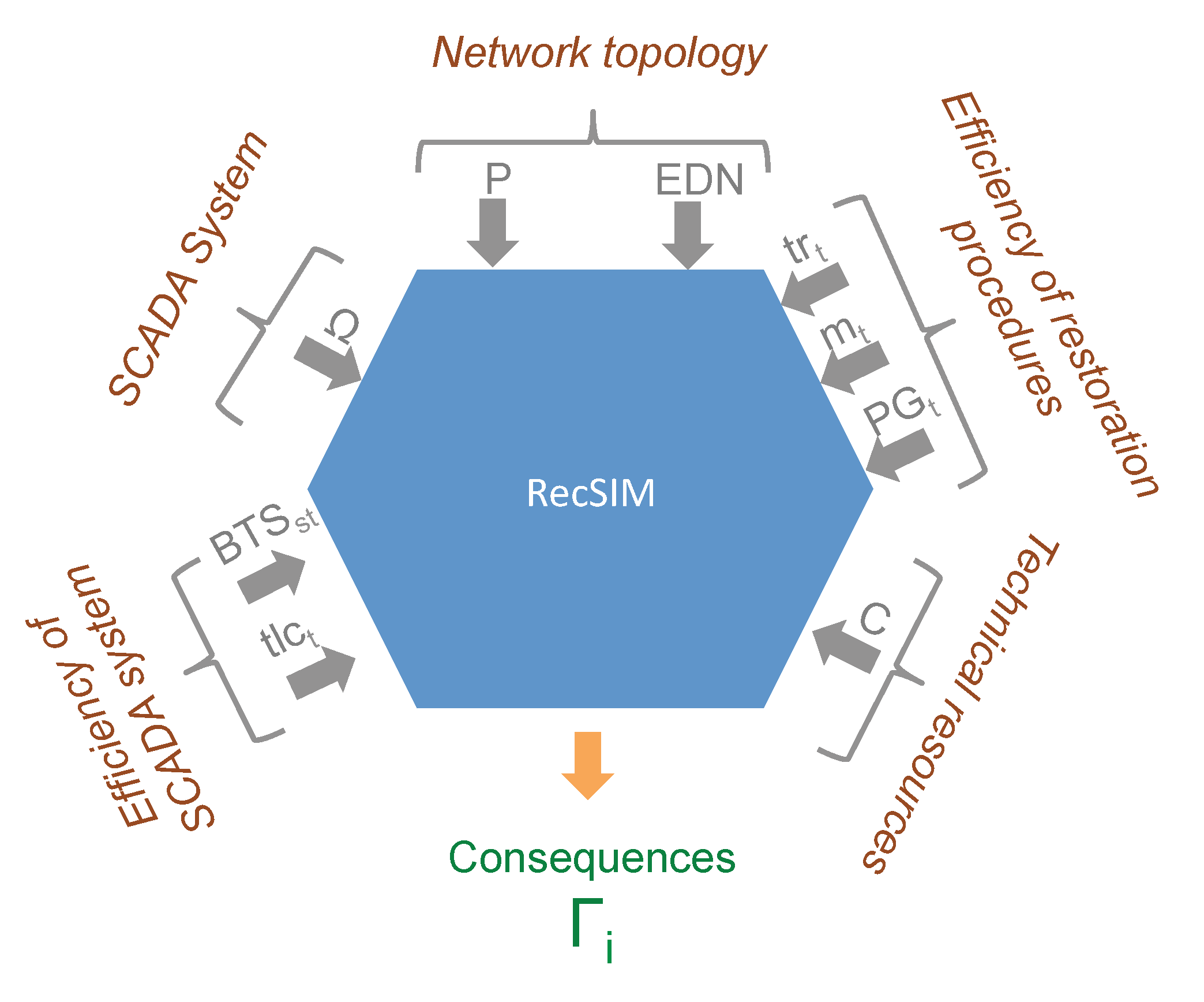
3. The RecSIM Tool
- Network topology—expressed as the EDN graph and the perturbation P represented by the SS is in the damaged state. In this work, perturbation P is introduced by the user. However, the node in the damaged state can also result from the analysis of external perturbation (i.e., weather forecast) and result from an over-threshold probability of damage of a node induced by a natural hazard (e.g., in the CIPCast platform, see [22,34]);
- SCADA system—expressed in terms of the set of SS that can be remotely tele-controlled;
- Efficiency of SCADA system—expressed in terms of the functioning status of the BTS providing communication service to the EDN and in terms of , the time needed to perform a remote operator action (using the EDN SCADA functionalities);
- Efficiency of restoration procedures—expressed in terms of the time needed by an emergency crew (a) to reach a damaged SS (), (b) to perform a manual reconnection action () and (c) to set in place a PG to feed the users of the damaged SS (or of other SS, which will result in being isolated and thus needing a PG as they were damaged). The input time values represent “mean” values as they have been provided by the electrical operator. RecSim performed simulations by using these values as mean values of a flat distribution from which time values to be used in the simulation were randomly extracted;
- Technical resources—expressed in terms of the number C of technical crews available in the field. The number of available PGs is assumed to constitute an unlimited resource. Further development of the algorithm will consider the finiteness of available PGs.
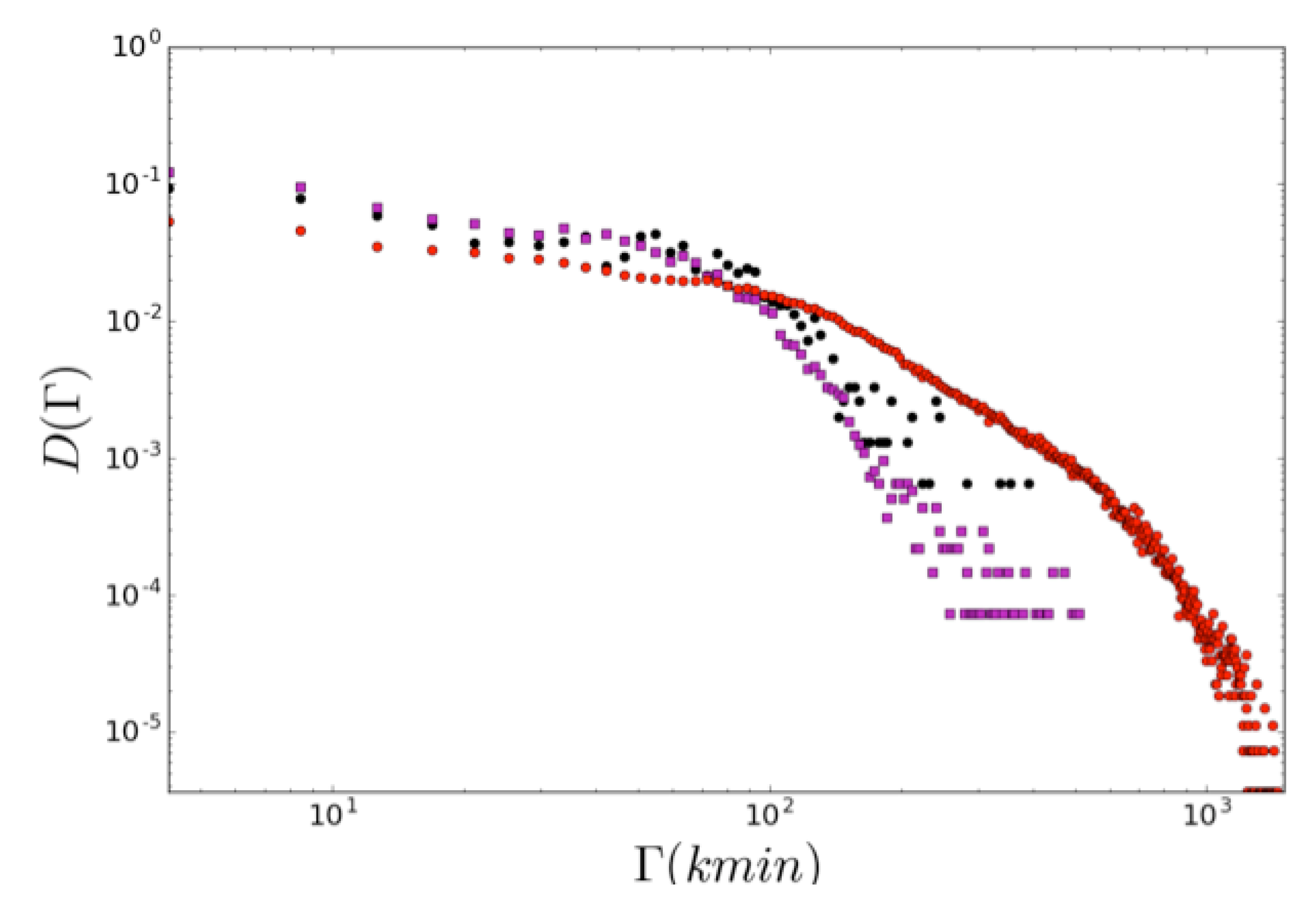
4. Assessing Robustness of Electrical Distribution Network Components and Possible Physical Damage Scenarios
5. Results
5.1. Resilience Assessment of EDN in Case of Metropolitan Contingency Scenarios
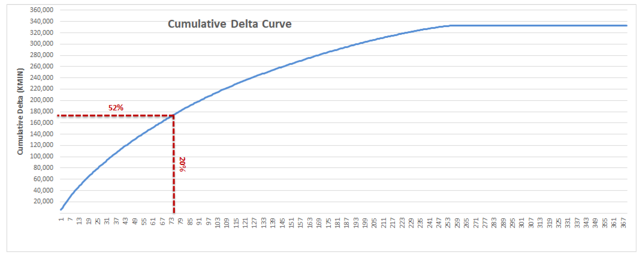
5.2. Electrical Distribution Network Sensitivity Analysis
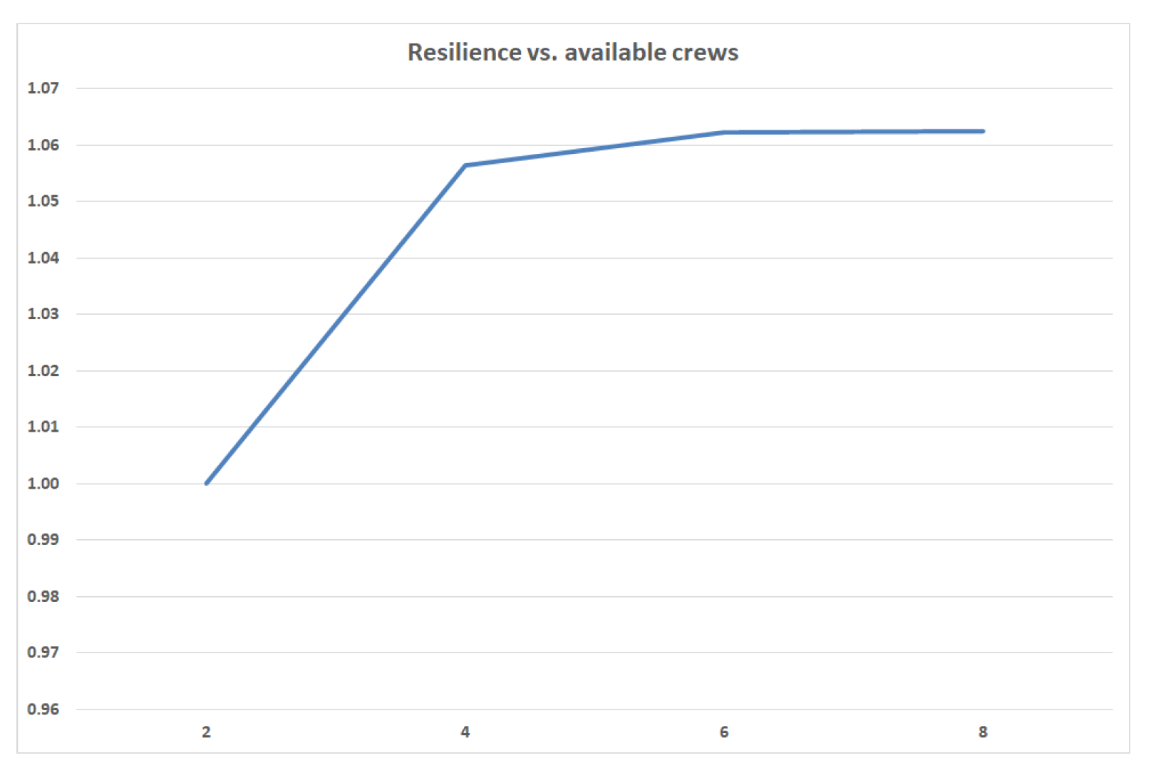
5.2.1. EDN Resilience vs. Number of Available Technical Crews
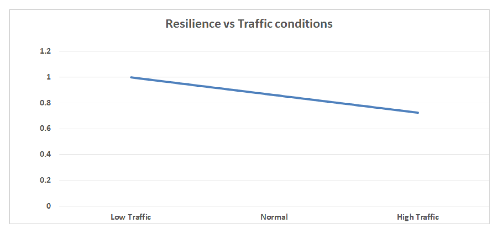
5.2.2. EDN Resilience vs. Traffic Congestion
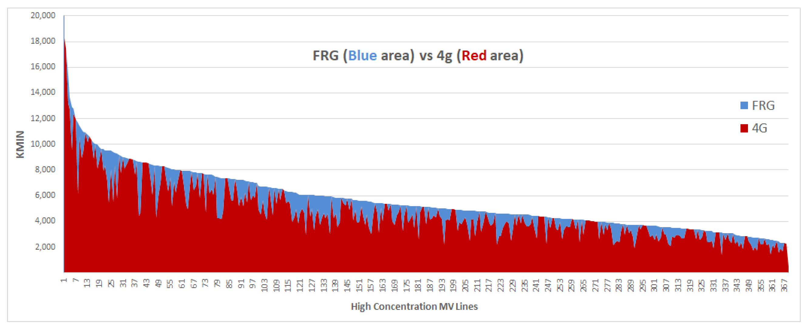
5.3. Assessing the Impact of Improved Distribution Automation Systems (DAS) on the EDN Resilience
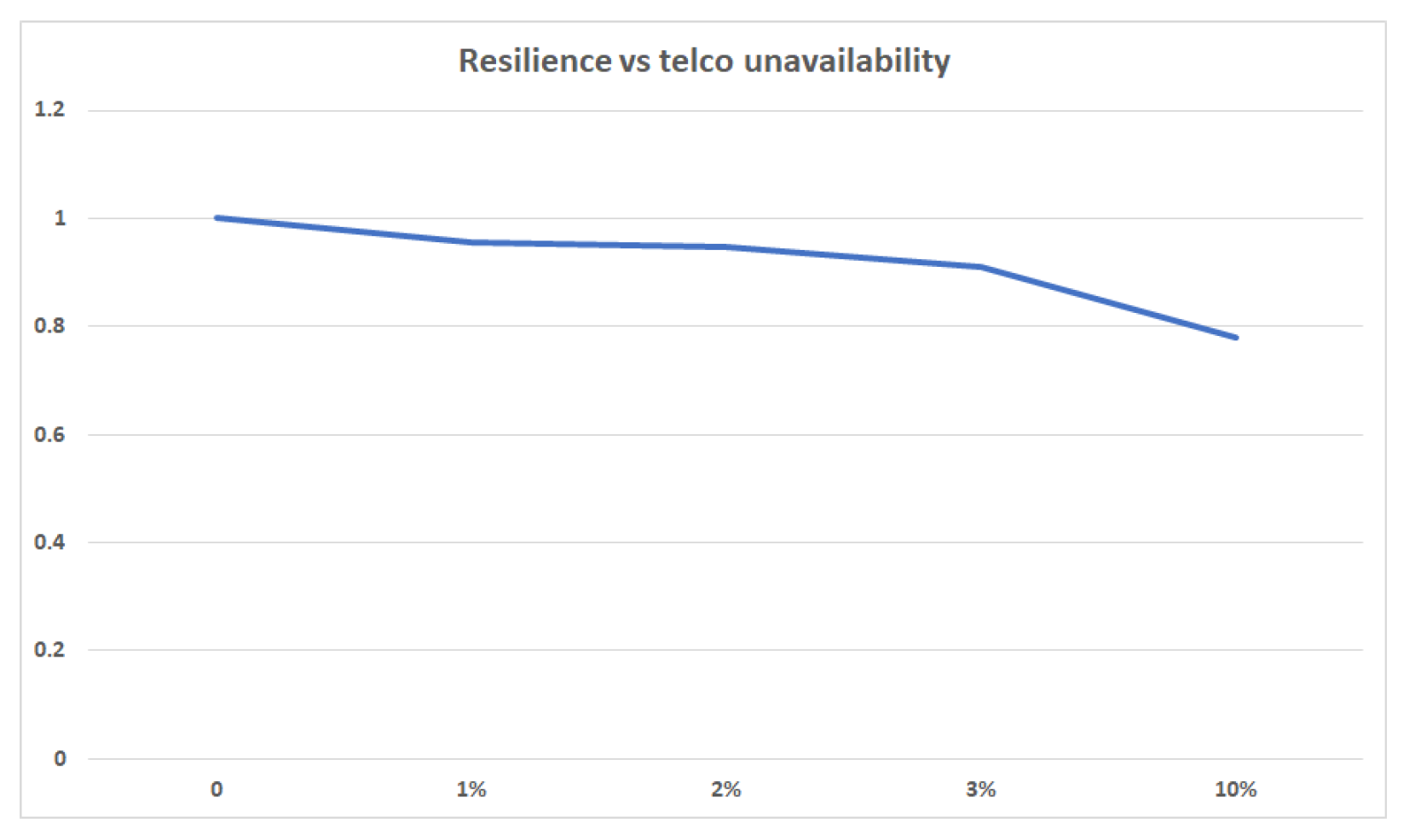
EDN Resilience vs. SCADA System Availability
6. Discussion
Author Contributions
Funding
Institutional Review Board Statement
Informed Consent Statement
Data Availability Statement
Acknowledgments
Conflicts of Interest
Abbreviations
| MDPI | Multidisciplinary Digital Publishing Institute |
| DOAJ | Directory of open access journals |
| TLA | Three letter acronym |
| LD | linear dichroism |
Appendix A
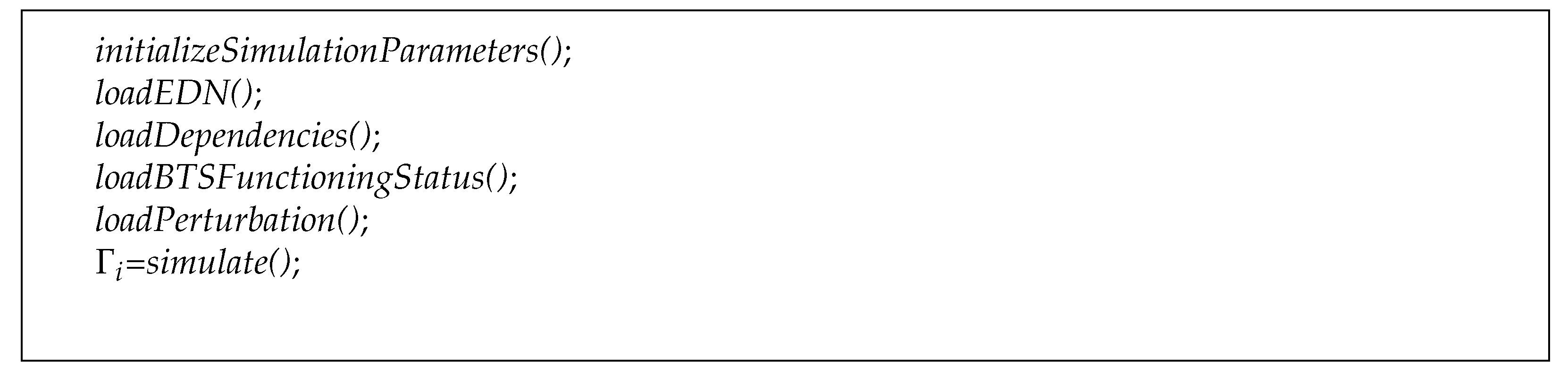

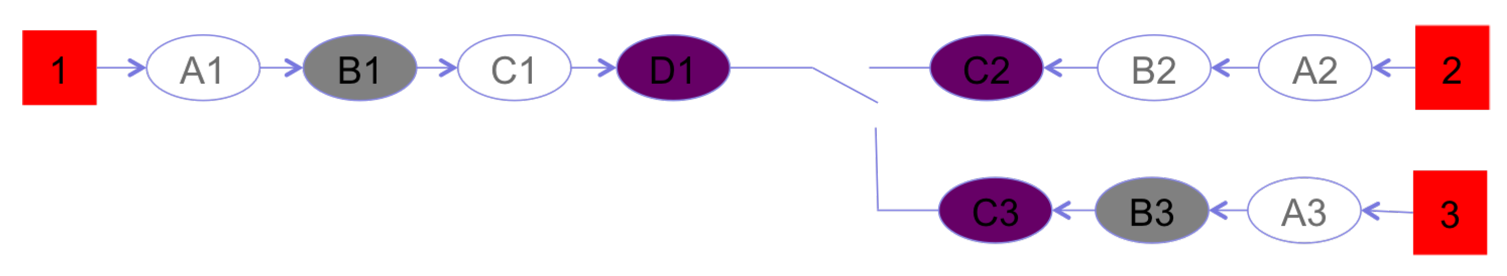
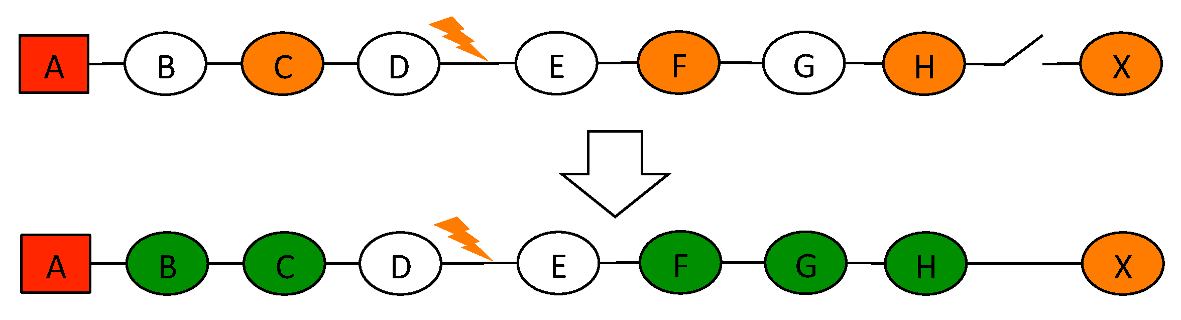
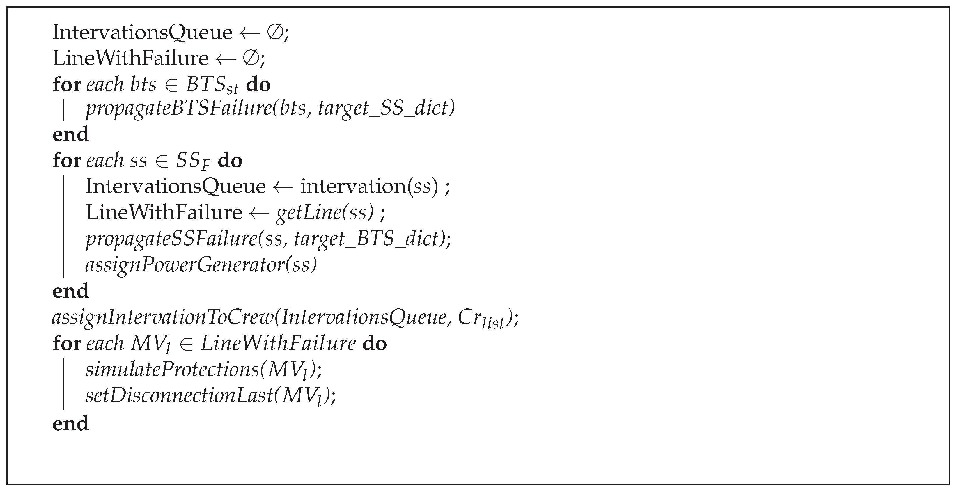
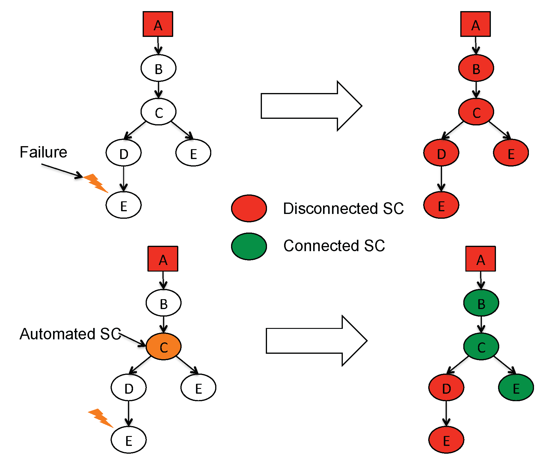
- the subtree contains automated secondary stations and at least one of these nodes belong to the path . Formally:If there are more of such automated nodes the simulateProtections() chooses the last automated node in the path (i.e., the nearest automated node to ). The procedure chooses the next node of this node in the path . Let us indicate this node with . Then, the procedure sets the status of all nodes belonging to the subtree rooted with () as disconnected;
- there are no automated nodes in the line. In this case the simulateProtections() sets the status of all nodes in as disconnected.

- The procedure checks if there exist tele-controlled nodes in the path . Let us assume that is the last tele-controlled node in this path and that the SCADA system is working properly. Then, the procedure computes the subtree obtained removing the outcoming edges from . The procedure sets the disconnection time of all the nodes in equal to (the mean time needed to perform a tele-controlled action). If there are no tele-controlled nodes in the path or their SCADA system is not working (because of BTS failures) the procedure sets the disconnection time to all nodes (where in this case, is obtained by removing the incoming edge to ) to , that is, the time that the technical crew needs to travel to the failed node and to perform the manual actions to isolate the failure.
- The procedure sets the disconnection time to all nodes of all subtrees obtained by removing the outcoming edges from . For each the procedure checks if there are frontier nodes in order to energize or part of it, using another MV line. In general, there are different cases:
- (a)
- There exists a frontier node (denoted by )that can be connected to another line and the related frontier node in has the functioning status (i.e., there are no failures and/or disconnections on ). Moreover, the connection of the two frontier nodes can be performed using the SCADA system. In this case, the procedure checks if there exist tele-controlled nodes in the path . Let us assume that is the first tele-controlled node in this path and that the SCADA system is working properly. Then, the procedure computes the subtree obtained, removing the incoming edge to . The procedure sets the disconnection time of all the nodes in equal to .
- (b)
- There exists a frontier node (denoted by )that can be connected to another line and the related frontier node in has the functioning status; however, the connection of the two frontier nodes has to be performed manually. In this case, the procedure assigns this new intervention to the technical crew, that can be available or not, to set the disconnection time of all node in according to the time needed to the technical crew to perform the operation.
- (c)
- There does not exist a frontier node. In this case, the nodes in are isolated and the disconnection time is set equal to , that is, the time needed to connect the node users to a mobile power generator.
- The procedure sets the disconnection time of node equal to .
- In steps 1 and 2, the procedure simulated all possible remotely controlled actions. In general, there remain a number of nodes that will be reconnected after manual isolation and restoration actions. The disconnection time of these nodes will be set accordingly.
- . In this case, the time needed to perform the manual operation is ;
- . In this case, manual operations will be performed in whilst the remaining interventions will be added, using a uniform work load criteria, to the intervention list of some emergency crew. For instance, if an intervention is added in the second position of the intervention list of a technical crew the time needed to perform this operation will be .
References
- Karagiannis, G.; Turksezer, Z.I.; Alfieri, L.; Feyen, L.; Krausmann, E. Climate Change and Critical Infrastructure —Floods. In EUR—Scientific and Technical Research Reports; Publications Office of the European Union: Luxembourg, 2017. [Google Scholar]
- ARERA. Increasing the Resilience of Electricity Transmission and Distribution Networks. Guideline. 2017. Available online: https://www.arera.it/allegati/docs/17/645-17eng_CapI.pdf (accessed on 29 November 2018).
- Kwasinski, A. Quantitative Model and Metrics of Electrical Grids: Resilience Evaluated at a Power Distribution Level. Energies 2016, 9, 93. [Google Scholar] [CrossRef]
- Willis, H.H.; Loa, K. Measuring the Resilience of Energy Distribution Systems; Technical Report; RAND Corporation: Santa Monica, CA, USA, 2015; Available online: https://www.rand.org/pubs/research_reports/RR883.html (accessed on 1 March 2018).
- Panteli, M.; Mancarella, P. Modeling and Evaluating the Resilience of Critical Electrical Power Infrastructure to Extreme Weather Events. IEEE Syst. J. 2017, 11, 1733–1742. [Google Scholar] [CrossRef]
- Bie, Z.; Lin, Y.; Li, G.; Li, F. Battling the Extreme: A Study on the Power System Resilience. Proc. IEEE 2017, 105, 1253–1266. [Google Scholar] [CrossRef]
- Lee, R.M.; Assante, M.J.; Conway, T. Analysis of the Cyber Attack on the Ukrainian Power Grid. Defense Use Case. 2016. Available online: https://media.kasperskycontenthub.com/wp-content/uploads/sites/43/2016/05/20081514/E-ISAC_SANS_Ukraine_DUC_5.pdf (accessed on 29 November 2018).
- Linkov, I.; Florin, M.V.; Trump, B. IRGC Resource Guide on Resilience. 2017. Available online: https://irgc.org/risk-governance/resilience/irgc-resource-guide-on-resilience/ (accessed on 8 June 2021).
- Haimes, Y.Y. On the Definition of Resilience in Systems. Risk Anal. 2009, 29, 498–501. [Google Scholar] [CrossRef]
- CIPedia. CIPRNet CIPedia. 2017. Available online: http://www.cipedia.eu (accessed on 1 March 2021).
- IMPROVER. IMPROVER Project. 2017. Available online: http://improverproject.eu (accessed on 1 March 2018).
- Bruneau, M.; Chang, S.; Eguchi, R.; Lee, G.; O’Rourke, T.; Reinhorn, A.; Shinozuka, M.; Tierney, K.; Wallace, W.; Winterfeldt, D. A Framework to Quantitatively Assess and Enhance the Seismic Resilience of Communities. Earthq. Spectra 2003, 19. [Google Scholar] [CrossRef] [Green Version]
- Hollnagel, E.; Pariès, J.; Woods, D.; Wreathall, J. Resilience Engineering in Practice: A Guidebook; CRC Press: London, UK, 2010. [Google Scholar]
- Nan, C.; Sansavini, G.; Kroger, W.; Heinimann, H. A quantitative method for assessing the resilience of infrastructure systems. In Proceedings of the PSAM 2012—Probabilistic Safety Assessment and Management, Honolulu, HI, USA, 22–27 June 2014. [Google Scholar]
- Filippini, R.; Silva, A. A modeling framework for the resilience analysis of networked systems-of-systems based on functional dependencies. Reliab. Eng. Syst. Saf. 2014, 125, 82–91. [Google Scholar] [CrossRef]
- Ganin, A.A.; Massaro, E.; Gutfraind, A.; Steen, N.; Keisler, J.M.; Kott, A.; Mangoubi, R.; Linkov, I. Operational resilience: Concepts, design and analysis. Sci. Rep. 2016, 6, 1–12. [Google Scholar] [CrossRef] [Green Version]
- Kong, J.; Simonovic, S.; Zhang, C. Resilience Assessment of Interdependent Infrastructure Systems: A Case Study Based on Different Response Strategies. Sustainability 2019, 11, 6552. [Google Scholar] [CrossRef] [Green Version]
- Ayyub, B.M. Systems Resilience for Multihazard Environments: Definition, Metrics, and Valuation for Decision Making. Risk Anal. 2014, 34, 340–355. [Google Scholar] [CrossRef]
- Zidan, A.; Khairalla, M.; Abdrabou, A.M.; Khalifa, T.; Shaban, K.; Abdrabou, A.; El Shatshat, R.; Gaouda, A.M. Fault Detection, Isolation, and Service Restoration in Distribution Systems: State-of-the-Art and Future Trends. IEEE Trans. Smart Grid 2017, 8, 2170–2185. [Google Scholar] [CrossRef]
- Zhang, H.; Yuan, H.; Li, G.; Lin, Y. Quantitative Resilience Assessment under a Tri-Stage Framework for Power Systems. Energies 2018, 11, 1427. [Google Scholar] [CrossRef] [Green Version]
- Abeysinghe, S.; Wu, J.; Sooriyabandara, M.; Abeysekera, M.; Xu, T.; Wang, C. Topological properties of medium voltage electricity distribution networks. Appl. Energy 2018, 210, 1101–1112. [Google Scholar] [CrossRef]
- Di Pietro, A.; Lavalle, L.; La Porta, L.; Pollino, M.; Tofani, A.; Rosato, V. Managing the Complexity of Critical Infrastructures. Studies in Systems, Decision and Control; Chapter Design of DSS for Supporting Preparedness to and Management of Anomalous Situations in Complex, Scenarios; Setola, R., Rosato, V., Kyriakides Rome, E., Eds.; Springer: Cham, Switzerland, 2016. [Google Scholar]
- Meerow, S.; Newell, J.P.; Stults, M. Defining urban resilience: A review. Landsc. Urban Plan. 2016, 147, 38–49. [Google Scholar] [CrossRef]
- McLellan, B.; Zhang, Q.; Farzaneh, H.; Utama, N.A.; Ishihara, K.N. Resilience, Sustainability and Risk Management: A Focus on Energy. Challenges 2012, 3, 153–182. [Google Scholar] [CrossRef] [Green Version]
- Aven, T. How some types of risk assessments can support resilience analysis and management. Reliab. Eng. Syst. Saf. 2017, 167, 536–543. [Google Scholar] [CrossRef]
- Stergiopoulos, G.; Kotzanikolaou, P.; Theocharidou, M.; Lykou, G.; Gritzalis, D. Time-based critical infrastructure dependency analysis for large-scale and cross-sectoral failures. Int. J. Crit. Infrastruct. Prot. 2016, 12, 46–60. [Google Scholar] [CrossRef]
- Giovinazzi, S.; Pollino, M.; Kongar, I.; Rossetto, T.; Caiaffa, E.; Pietro, A.D.; Porta, L.L.; Rosato, V.; Tofani, A. Towards a Decision Support Tool for Assessing, Managing and Mitigating Seismic Risk of Electric Power Networks. In Lecture Notes in Computer Science, Proceedings of the Computational Science and Its Applications—ICCSA 2017, Trieste, Italy, 3–6 July 2017; Gervasi, O., Ed.; Springer: Cham, Switzerland, 2017; Volume 10406. [Google Scholar] [CrossRef]
- D’Agostino, G.; Pietro, A.D.; Giovinazzi, S.; Porta, L.L.; Pollino, M.; Rosato, V.; Tofani, A. Earthquake Simulation on Urban Areas: Improving Contingency Plans by Damage Assessment. In Lecture Notes in Computer Science, Proceedings of the Critical Information Infrastructures Security (CRITIS 2018), Kaunas, Lithuania, 24–26 September 2018; Luiijf, E., Žutautaitė, I., Hämmerli, B., Eds.; Springer: Cham, Switzerland, 2018; Volume 11260. [Google Scholar] [CrossRef]
- Tofani, A.; D’Agostino, G.; Di Pietro, A.; Onori, G.; Pollino, M.; Alessandroni, S.; Rosato, V. Operational Resilience metrics for a complex electrical network. In Proceedings of the CRITIS 2017, Lucca, Italy, 8–13 October 2017. [Google Scholar] [CrossRef]
- Tofani, A.; D’Agostino, G.; Di Pietro, A.; Giovinazzi, S.; La Porta, L.; Parmendola, G.; Pollino, M.; Rosato, V. Infrastructure Management and Construction. In Infrastructure Management and Construction; Chapter Modeling Resilience in Electrical Distribution Networks; Sepasgozar, S.M.E., Tahmasebinia, F., Shirowzhan, S., Eds.; IntechOpen: London, UK, 2019; Available online: https://www.intechopen.com/books/infrastructure-management-and-construction/modeling-resilience-inelectrical-distribution-networks (accessed on 15 April 2021).
- Popovic, Z.N.; Knezevic, S.D.; Popović, D.S. Risk-Based Allocation of Automation Devices in Distribution Networks With Performance-Based Regulation of Continuity of Supply. IEEE Trans. Power Syst. 2019, 34, 171–181. [Google Scholar] [CrossRef]
- Lim, I.; Ha, B. An optimal composition and placement of automatic switches in DAS. In Proceedings of the 2016 IEEE Power and Energy Society General Meeting (PESGM), Boston, MA, USA, 17–21 July 2016. [Google Scholar]
- Sun, L.; You, S.; Hu, J.; Wen, F. Optimal Allocation of Smart Substations in a Distribution System Considering Interruption Costs of Customers. IEEE Trans. Smart Grid 2018, 9, 3773–3782. [Google Scholar] [CrossRef] [Green Version]
- Tofani, A.; Di Pietro, A.; Lavalle, L.; Pollino, M.; Rosato, V. CIPRNet decision support system: Modelling electrical distribution grid internal dependencies. In Proceedings of the Critical Infrastructures Preparedness: Status of Data for Resilience Modelling, Simulation and Analysis (MS&A), ESReDA Workshop, Wroclaw, Poland, 28–29 May 2015. [Google Scholar]
- Calcara, L.; Pietro, A.D.; Giovinazzi, S.; Pollino, M.; Pompili, M. Towards the Resilience Assessment of Electric Distribution System to Earthquakes and Adverse Meteorological Conditions. In Proceedings of the 2018 AEIT International Annual Conference, Bari, Italy, 3–5 October 2018; pp. 1–6. [Google Scholar]
- Giovinazzi, S.; Pollino, M.; Tofani, A.; Pietro, A.D.; Porta, L.L.; Rosato, V. A Decision Support System for mitigating the seismic risk of electric distribution networks: Learnings from the Central Italy earthquake sequence 2016–2017. In Proceedings of the 2019 AEIT International Annual Conference (AEIT), Florence, Italy, 18–20 September 2019; pp. 1–6. [Google Scholar]
- Diao, K.; Sweetapple, C.; Farmani, R.; Fu, G.; Ward, S.; Butler, D. Global resilience analysis of water distribution systems. Water Res. 2016, 106. [Google Scholar] [CrossRef] [Green Version]
- Lavalle, L.; Patriarca, T.; Daulne, B.; Hautier, O.; Tofani, A.; Ciancamerla, E. Simulation-Based Analysis of a Real Water Distribution Network to Support Emergency Management. IEEE Trans. Eng. Manag. 2020, 67, 554–567. [Google Scholar] [CrossRef]
- Di Nardo, M.; Clericuzio, M.; Murino, T.; Madonna, M. An Adaptive Resilience Approach for a High Capacity Railway. Int. J. Civ. Eng. 2020, 10. [Google Scholar] [CrossRef]
- Liu, X.; Ferrario, E.; Zio, E. Resilience Analysis Framework for Interconnected Critical Infrastructures. ASME J. Risk Uncertain. Part B 2017, 3. [Google Scholar] [CrossRef]
- Khan, M.T.; Shrobe, H. Security of Cyberphysical Systems: Chaining Induction and Deduction. Computer 2019, 52, 72–75. [Google Scholar] [CrossRef]
- Lou, X.; Tellabi, A. Cybersecurity Threats, Vulnerability and Analysis in Safety Critical Industrial Control System (ICS). In Recent Developments on Industrial Control Systems Resilience; Springer: Cham, Switzerland, 2020; pp. 75–97. [Google Scholar] [CrossRef]


| EDNs Exposed Components | Type | Vulnerability Factors | Damage Metric |
|---|---|---|---|
| Generators | Node | Building characteristics (geometry, node typology, earthquake resistant design (ERD). Internal elements characteristics (i.e., type of anchoring). | Damage level |
| Primary and Secondary Substations | Node | Dedicated or multipurpose structure. Building characteristics (geometry, typology, earthquake resistant design (ERD)). Internal elements characteristics (i.e., type of anchoring). | Damage level |
| Buried power lines | Line | Cables and conductors: material, geometrical characteristics (diameter and length measured between joints). Joints: constructive characteristics. | Damage frequency |
| Aerial power lines, cables and electric conductors | Line | Cables and conductors: material, geometrical characteristics. Poles: material, height, foundations type. Support structures: material, type. Insulators: terminal block type. | Damage frequency |
| Aerial power lines and switch disconnectors | Node on aerial line | Height above ground. Switch disconnectors mass. Anchor type. Aerial line shelf type. | Damage level |
| Aerial power lines and transformer/substations located on a pole | Node on aerial line | Height above ground. Transformer weight. Anchor type. Shelf type. | Damage level |
| Model Parameters S1 Simulations | |
|---|---|
| network topology | normal configuration |
| number of technical crews available on the field | |
| time for tele-control operation () | min |
| time for technical intervention on-site () | min |
| time for installing an electrical generator () | min |
| fraction of tele-controllable SS being not tele-controllable | |
| Model Parameters S2 Simulations | |
|---|---|
| network topology | normal configuration |
| number of technical crews available on the field | 4 |
| time for tele-control operation () | min |
| time for technical intervention on-site () | min |
| time for installing an electrical generator () | min |
| fraction of tele-controllable SS being not tele-controllable | |
| Model Parameters S3 Simulations | |
|---|---|
| network topology | normal configuration |
| number of technical crews available on the field | 4 |
| time for tele-control operation () | min |
| time for technical intervention on-site () | min |
| time for installing an electrical generator () | min |
| fraction of tele-controllable SS being not tele-controllable | |
| Model Parameters S4 Simulations | |
|---|---|
| network topology | normal configuration |
| number of technical crews available on the field | 4 |
| time for tele-control operation () | min |
| time for technical intervention on-site () | min |
| time for installing an electrical generator () | min |
| fraction of tele-controllable SS being not tele-controllable | |
Publisher’s Note: MDPI stays neutral with regard to jurisdictional claims in published maps and institutional affiliations. |
© 2021 by the authors. Licensee MDPI, Basel, Switzerland. This article is an open access article distributed under the terms and conditions of the Creative Commons Attribution (CC BY) license (https://creativecommons.org/licenses/by/4.0/).
Share and Cite
Tofani, A.; D'Agostino, G.; Di Pietro, A.; Giovinazzi, S.; Pollino, M.; Rosato, V.; Alessandroni, S. Operational Resilience Metrics for Complex Inter-Dependent Electrical Networks. Appl. Sci. 2021, 11, 5842. https://doi.org/10.3390/app11135842
Tofani A, D'Agostino G, Di Pietro A, Giovinazzi S, Pollino M, Rosato V, Alessandroni S. Operational Resilience Metrics for Complex Inter-Dependent Electrical Networks. Applied Sciences. 2021; 11(13):5842. https://doi.org/10.3390/app11135842
Chicago/Turabian StyleTofani, Alberto, Gregorio D'Agostino, Antonio Di Pietro, Sonia Giovinazzi, Maurizio Pollino, Vittorio Rosato, and Silvio Alessandroni. 2021. "Operational Resilience Metrics for Complex Inter-Dependent Electrical Networks" Applied Sciences 11, no. 13: 5842. https://doi.org/10.3390/app11135842
APA StyleTofani, A., D'Agostino, G., Di Pietro, A., Giovinazzi, S., Pollino, M., Rosato, V., & Alessandroni, S. (2021). Operational Resilience Metrics for Complex Inter-Dependent Electrical Networks. Applied Sciences, 11(13), 5842. https://doi.org/10.3390/app11135842