Abstract
The aim of this work was to provide a formulation of a non-linear diffusion model with forced convection in the form of a reaction–absorption system. The model was studied with analytical and numerical approaches in the frame of the parabolic operators theory. In addition, the solutions are applied to a gas interaction phenomenon with the intention of producing an inerted ullage in an Airbus A320 aircraft centre fuel tank. We made use of the travelling wave (TW) solutions approach to study the existence of solutions, stability and the precise evolution of profiles. The application exercise sought to answer a key question for aerospace sciences which can be formulated as the time required to ensure an aircraft fuel tank is safe (inerted) to prevent explosion due to the presence of oxygen in the tank ullage.
Keywords:
non-linearity; reaction; absorption; coupled system; gas interaction; inerting; aircrafts; fuel tank; travelling waves 1. Introduction
In the 1930s, Fisher [1], proposed a reaction–diffusion model to describe the interactive dynamic of genes. In parallel, Kolmogorov, Petrovskii and Piskunov [2] proposed the same equation in combustion theory. In both cases, the models considered a Gaussian order two-diffusion model with a non-linear reaction of the form . The authors introduced the concept of travelling wave (TW) solutions to describe the propagation features of each involved species. Afterwards, the Fisher–KPP model was subjected to remarkable mathematical research to explore further applications (see [3,4,5]). More recently, some analyses [6] have shown new patterns of formation in chemistry and biology (compared to those existing in the current literature, see the remarkable references [7,8]) for travelling waves solutions and making use of numerical algorithms.
The aim of this paper was to define a model and obtain results to predict the behaviour of interacting gases in a global medium with forced convection (advection) and diffusion. The gas interacting process, aimed to model, consists of the removal of oxygen from a fuel tank to prevent any hydrocarbon combustion in the case a generated spark or hot spot occurs [9]. One of the technical solutions raised for this purpose is known as an inerting system, which shall be understood as a fire preventive [10]. As a short description, the inerting system consists of a filter or membrane that separates the nitrogen and oxygen in the air. The nitrogen is introduced into the fuel tank while the oxygen is expelled outwards. The inerted atmosphere prevents the fire propagation as there is not sufficient oxygen concentration to produce and sustain a combustion process.
One possibility to model the nitrogen–oxygen interaction is to consider the nitrogen replacement by oxygen in the fuel tank air space. In [11], the authors developed an algebraic model based on a mass balance to determine the oxygen and nitrogen concentrations in fuel tank bays. Additionally, in [12], the algebraic model was compared with a transport differential equation based on a mass balance in a differential tank element. In both cases, the modelling exercise does not introduce diffusion into the interacting species, although the forced convection is introduced by the transport (in the sense of particle movement) phenomenon modelled.
The diffusion in the fuel tank was introduced by Ghadirian et al. [13] for simulating the interactive process of fuel vapours in a fuel tank. Such diffusion was proposed to be governed by the classical parabolic homogeneous equation:
where is the fuel concentration in the air, and z is the vertical coordinate. This problem considers only the diffusion, disregarding the natural convection terms and reaction or absorption phenomenon. The intention of this paper was to consider the forced convection together with a proposed interaction between the substances in the fuel tank.
2. Materials and Methods
The methods followed along this research were based on a hybrid assessment, analytical and numerical, together with a validation exercise with real testing data. The modelling set of equations were obtained based on the mass conservation principles.
The nitrogen gas was supplied by a manifold with several nozzles located along the fuel tank (see [14] for a complete description). The gases were dynamic together with the nitrogen nozzle location and the particular tank geometries led to an heterogeneous gas distribution along the tank. This heterogeneous condition has been modelled considering the stratified two-phase flows in [15], making use of the volume of fluid (VOF) model (see [16,17] for a detailed description) by solving the phase continuity equation. In the modelling exercise developed in this paper, it was considered that the heterogeneous nitrogen discharge in complex tank geometries provoked gas dispersion. As a consequence, a diffusion process emerges in response to the differences in the gas concentration along the tank zones. The selection of an appropriate diffusion principle is of relevance and leads to a whole significant discussion (see [18] and the references therein). For our purposes, the considered set of equations is non-linear in general and aims to characterize the propagation of the interacting gases. Such interactions are of significance in tank zones not influenced by the advection, so that the nitrogen propagates by diffusion. This progressive propagation in a diffusive front has been used for modelling purposes in other fields to simulate porosity effects [19,20]. In our case, the propagation dynamic was conceived as an inherent feature introduced by the travelling waves solutions.
In addition to the diffusion, the rate of nitrogen discharge along the domain induces a forced convection within the tank airspace.
To obtain the modelling equations, we consider the following dynamics between the nitrogen concentration (N) and the oxygen concentration (): initially, the fuel tank ullage is not saturated with nitrogen, so it is considered that the nitrogen time rate () is high. As long as the nitrogen concentration increases, the oxygen is expelled and the nitrogen time rate decreases. Then:
where shall be obtained for each particular case. In the same manner, the oxygen concentration decreases for increasing nitrogen quantities:
The expressions (2) and (3) will be referred to as the reaction () and absorption () in the modelling set of equations
Note that both the nitrogen and oxygen are functions of space and time and for , (, in this case).
Consider a virtual domain within the fuel tank . The mass conservation principle establishes that the time rate of nitrogen and oxygen concentrations () shall be equal to the concentration flux through the boundaries of () plus the absorption or reaction that act as independent terms.
We admit that the vectors and are the concentration fluxes along the boundary () per unit of area and per unit of time through the borders of the sub-domain . Consider the vector as the normal local at any point of . We admit that the absorption and reaction terms per unit of time and volume are given by the generic functions for the nitrogen and for the oxygen.
Each , , , is continuous with continuous derivatives. Therefore, for sufficiently continuous initial data, i.e., in the domain, the evolving solutions and are continuous and smooth (Chapter 7 [21]) in virtue of the regular parabolic spatial operator that adopts the Laplacian form as it will be shown. Then:
The Fick law [21] enables us to account for an expression to the vector fluxes:
The diffusion between the two interacting species requires that . Note that the vector introduces the advection term to account for the forced convection within the fuel tank. Hence:
Note that:
So that:
The initial concentrations of nitrogen and oxygen are mathematically given by constant homogeneous distributions, i.e., :
Considering the above information, the following problem P is formulated:
The operator’s parabolic regularity ensures the monotone evolution of each of the involved solutions (referring to Chapter 7 [21]). The decreasing and increasing condition of the solutions are, then, given by the reaction (increasing) and absorption terms (decreasing). As a consequence and preliminary, the nitrogen concentration N increases while the oxygen concentration decreases. Then, and upon evolution, the solutions will satisfy , which means that the total concentration of each substance does not blow up in the domain due to the non-linearity proposed in the reaction and absorption terms.
The problem P was introduced as a baseline model to account for the different terms involved in the gases dynamics. Now, a new problem is defined accordingly to account for the asymptotic behaviour of each of the substances. As it will be shown in Section 3.3, the fuel tank inerting process tends towards stationary values for the oxygen and nitrogen concentrations. This fact leads to consider travelling waves (TW) solutions connecting two stationary concentrations, both given by the initial and the asymptotic values. Mathematically, such solutions can be modelled by a Fisher–KPP reaction type. Consequently, the new problem in the TW domain is:
where is the asymptotic solution to N. If the initial data are constant, the same condition is expressed as .
The kinematic boundary condition related to the non-slip suggests that the velocity variations are located closed to the tank walls, while far from such borders, the described dynamic behaves free with minor influence of the boundary conditions. In addition, a dedicated description of the involved gases kinematic is out of the analysis scope; nonetheless, the influence and behaviour of the convective effects (through the vector a) are considered, and particularly, so is the effect of such advection into the gases concentrations . Thus, the intention is to study the dynamic associated with the solutions at the core of the domain (sufficiently large as to consider ) not affected by the domain borders.
3. Discussions and Results
3.1. Analysis in the Travelling Waves (TW) Domain
Solutions to problem (15) tend to equilibrium solutions upon evolution. Such equilibrium conditions are given by the technological limits and other environmental variables (see Section 3.3). In addition, note that the increasing monotone behaviour in the nitrogen leads to while for the oxygen that is expelled out of the tank. Then, the equilibrium condition for the nitrogen is expressed as
The oxygen concentration decreases so as to reach an asymptotic value close to the null equilibrium: .
To understand the involved dynamic and permit the analysis of TW evolutions, the initial conditions are given by a step function of Heaviside type:
The main objective is to determine the nitrogen and oxygen concentrations starting from the given initial data and evolving to the equilibrium solutions in the TW domain. Note that the step-like initial data permit us to analyse the behaviour for positive and null initial masses, as both are defined in the x intervals of a Heaviside function, i.e., for and for . Along this section, solutions are obtained making use of hybrid analytical and numerical evidence.
3.2. TW Profiles
TW solutions are obtained as , where d is a unitary vector in the TW direction, corresponds to the TW-speed and is the TW profile. Note that TW profiles are equivalent under translation and symmetry . We admit the vector in the TW propagation direction is expressed as and the TW moves from to ∞. Hence:
After replacement and standard operations, the problem (15) reads:
Note that the TW profile asymptotically tends towards zero whilst keeping the positivity condition. In addition, increases to , so that . These particular behaviours will be shown afterwards, but shall be taken into account during the coming assessments.
A linearisation of (19) close to the equilibrium condition is difficult in general due to the non-Lipschitz character of . Note that close to the critical point , , hence, the following alternative problem is formulated: (19):
TW profiles resulting from (20) are lower solutions to (19). This statement will be shown afterwards, but it is relevant to ensure the positivity of any TW profile. Indeed, any positive solution to (20) will provide evidence to ensure the positivity of any upper solution in (19).
Considering , then:
With the boundary conditions expressing the asymptotic behaviour of solutions:
The fundamental TW problem consist of finding a positive and monotone profile for a certain interval of TW speeds. Particularly, solutions are expressed in the proximity of the equilibrium points and . When solutions approach the boundary conditions in (22), a linearisation approach can be followed, so that solutions can be exponentially expressed as
Then, (21) reads:
From the second identity, it is possible to find an expression to relate the given speeds (TW speed and advection terms) with the exponential factor:
Similarly, for :
Note that for , the term , then:
Observe that the results for and establish that the exponential decaying terms are bigger than the advection and TW-speed terms . Hence, any TW profiles evolves towards the asymptotic equilibrium and this evolution is convergent, independently of the advection and TW speed terms.
Note that the existence, uniqueness and comparison of solutions to problems (19) and (20) follow a standard procedure, as proposed in [21] (Chapter 7). Along the following analysis, a numerical exercise is considered to provide particular forms of TW solutions to problem (19). Furthermore, solutions to (20), close to the critical points , are effectively shown to be lower solutions to (19). As solutions to problem (20) are lower compared with solutions to (19), a monotone (increasing or decreasing) TW profile and tip exist. The numerical exercise has been pursued with the following features:
- The methodology is based on the Matlab function bvp4c which provides an implicit Runge–Kutta approach with an interpolant extension [22]. The collocation method requires the specification of boundary conditions, in this case, given by the stationary solutions at and ;
- The integration interval is , large enough to study the TW evolution in their domain, and not impacted by the boundary conditions that act as tractors;
- The considered error for computation is ;
- The integration domain has been divided into 100,000 nodes;
- To make the numerical assessment tractable and without loss of generality, particular values were taken for the involved parameters: , —and different values of n and m.
Results are represented in Figure 1, Figure 2, Figure 3, Figure 4 and Figure 5 with the following remarks:
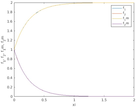
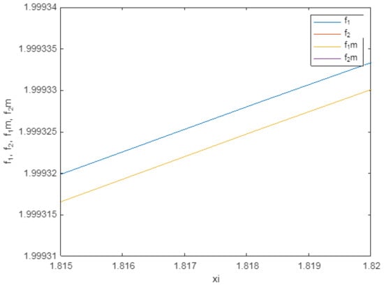
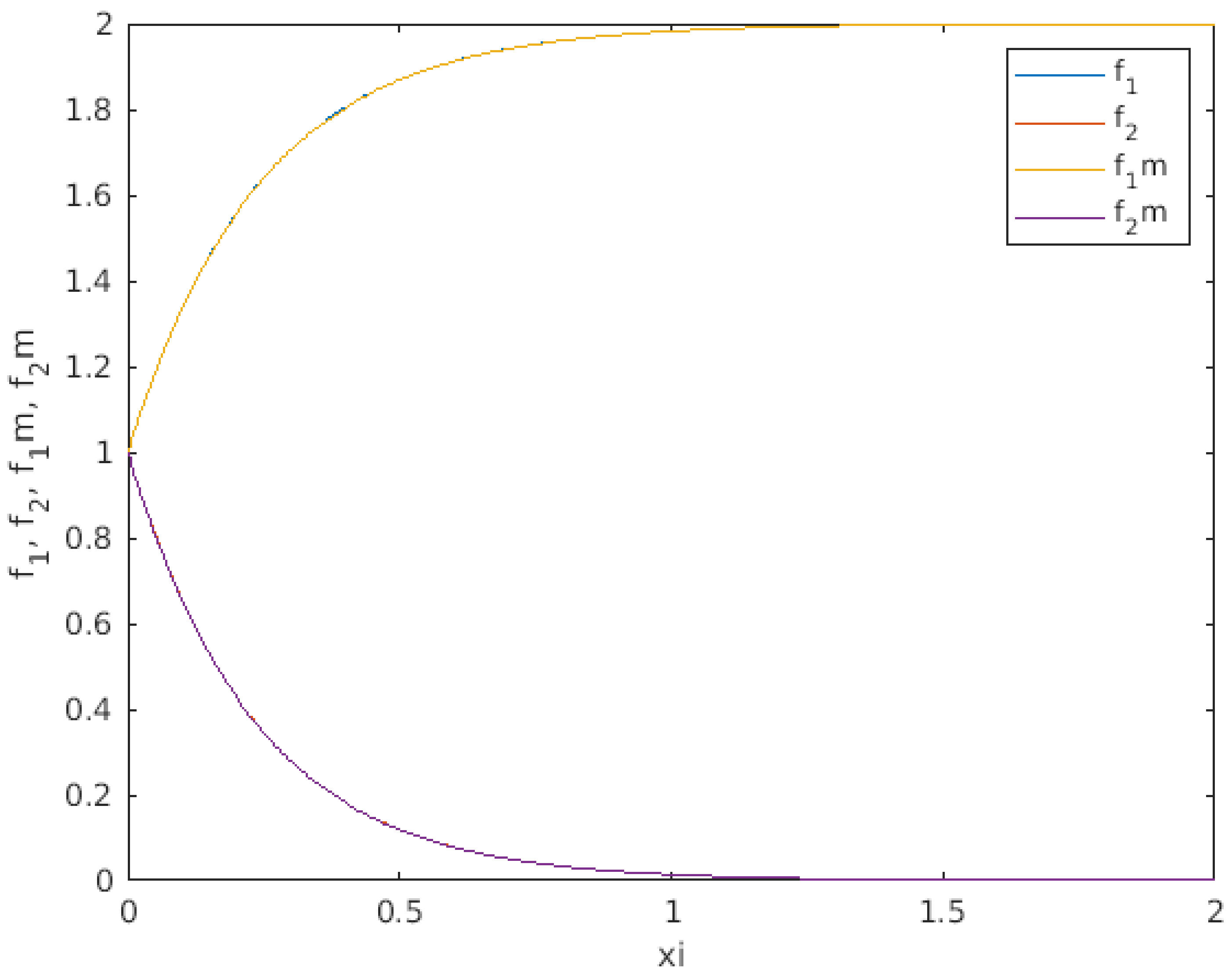
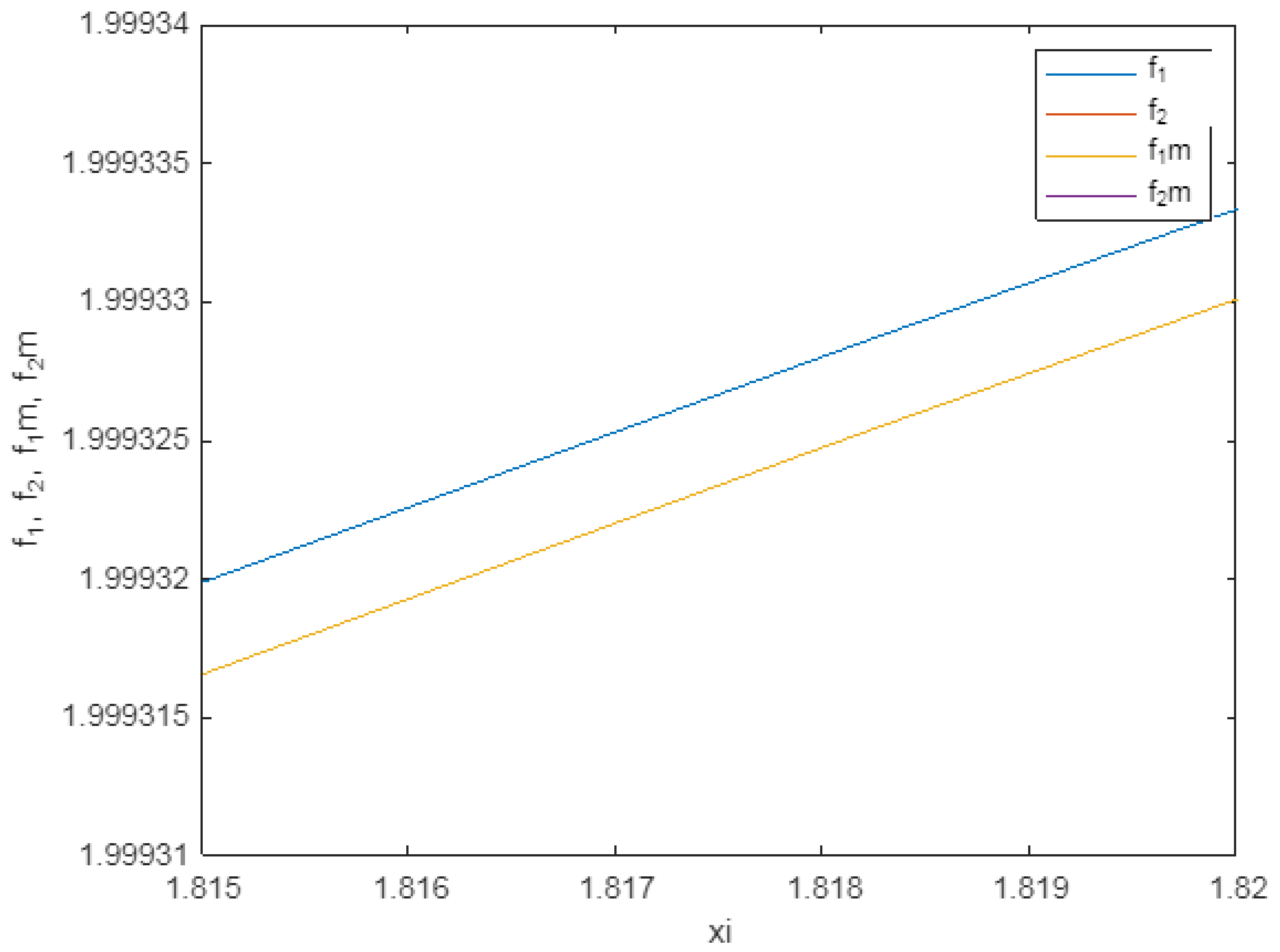
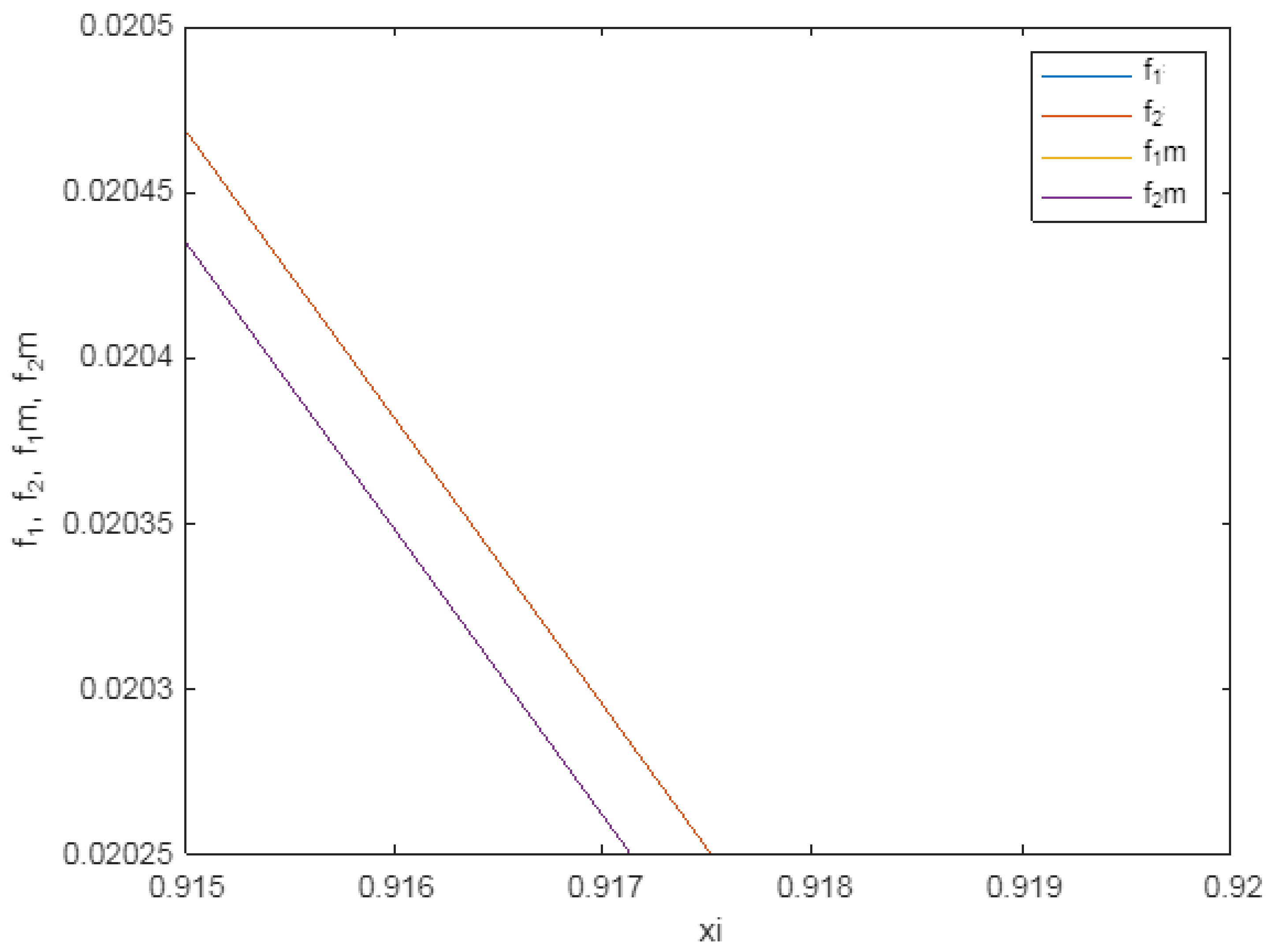
Figure 2.
TW profiles for with , . For the sake of simplicity, . Note the lower solution as the solution for the problem (20). The numerical exercise was performed for an integration interval ; nonetheless, the interval was cut for representation purposes. Note that and represent and solutions to (19) while and are solutions to (20).
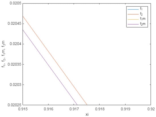
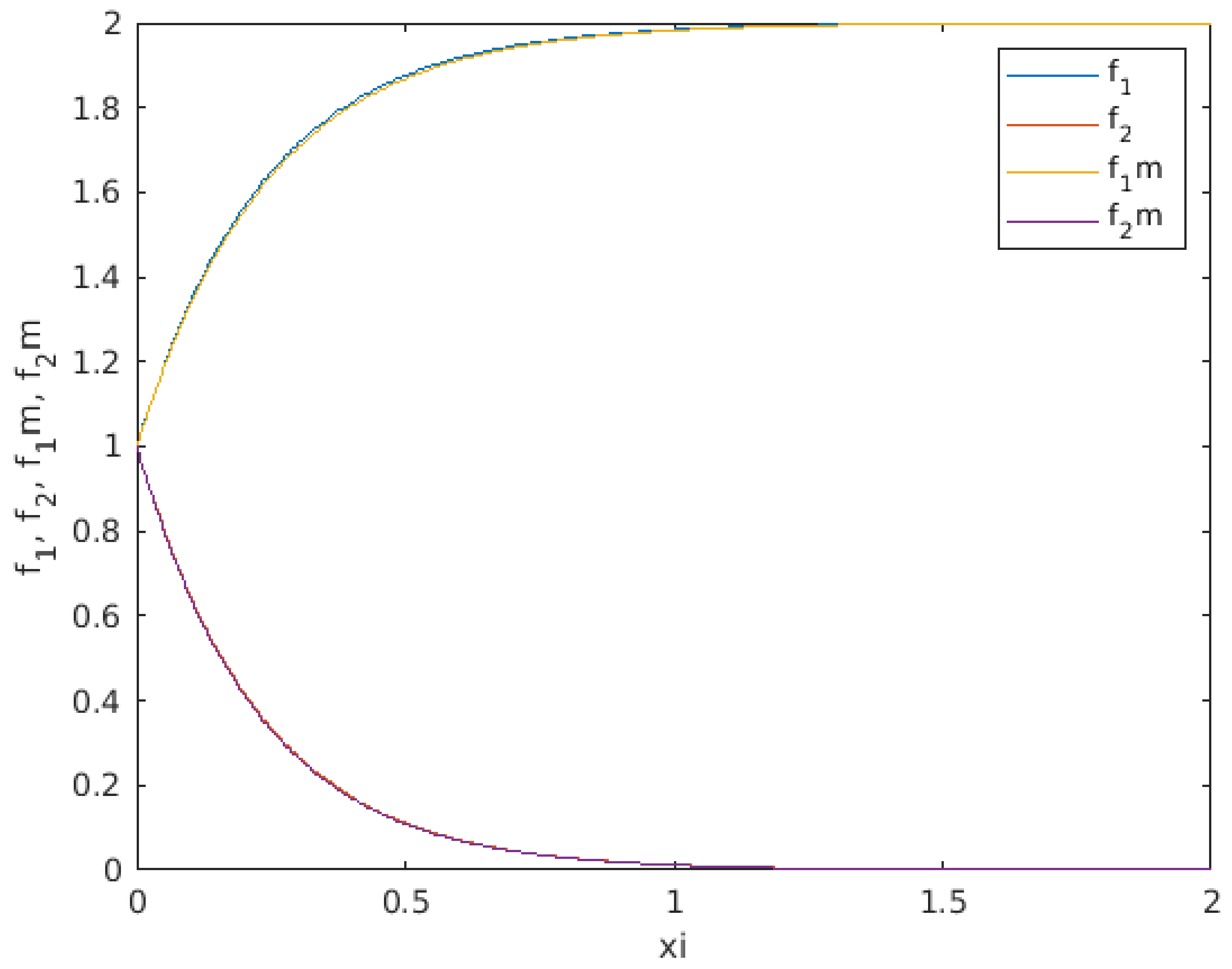
Figure 3.
TW profiles for with , . For the sake of simplicity, . Note the lower solution as the solution for the problem (20). The numerical exercise was performed for an integration interval ; nonetheless, the interval was cut for representation purposes. Note that and represent and solutions to (19) while and are solutions to (20).
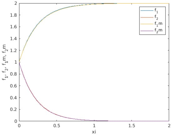
Figure 4.
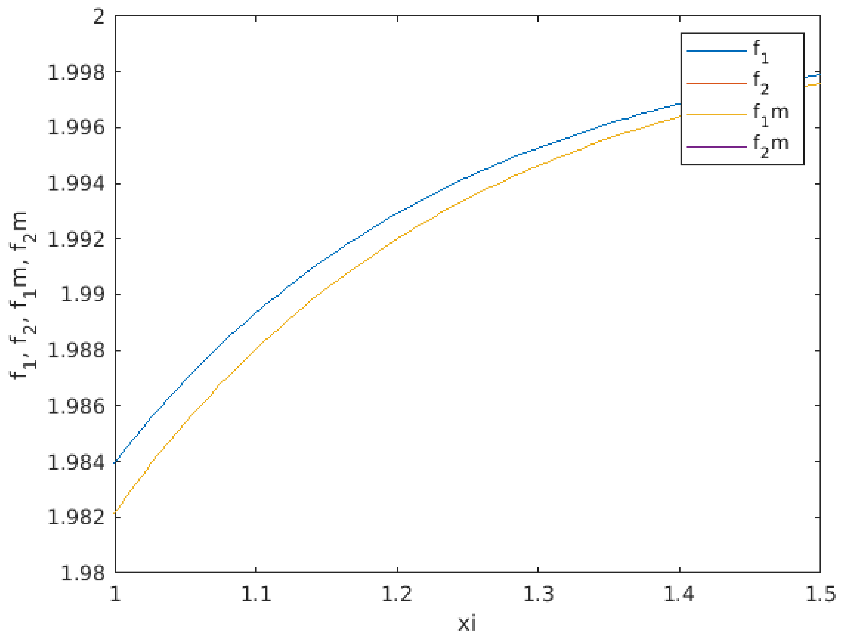
TW profiles for with , . For the sake of simplicity, . The numerical exercise was performed for an integration interval ; nonetheless, the interval was cut for representation purposes.
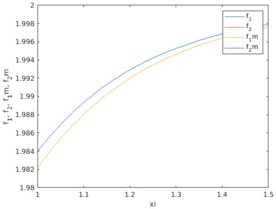
Figure 5.
TW profiles for with , . Note that the solution to (20) is represented by in the graph.
- Case with and —according to the results in Figure 1, Figure 2 and Figure 3, TW profiles to (20) are lower solutions compared to those for (19). Note that (as solution to (20)) is positive along the domain. Then, any TW moving with the exponential decaying term as per (25) is positive in the whole domain. In addition, we note that the solutions to (19) are very close to solutions to the linearised (20), which permits the validation of the goodness of the linearised exercise;
3.3. Application to a Fuel Tank Inerting Process
The phenomenon under study is related to the interaction between substances, i.e., the oxygen and the nitrogen in an aircraft fuel tank to generate an inert gas ullage. The model in Problem P has three different parameters that need to be determined, making use of real flight testing activities. Such flight test data are extracted from [14] and summarized in Figure 6. Note that for the particular oxygen sampling location, we refer the reader to the discussion in the sourced reference [14].
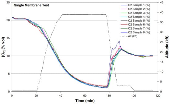
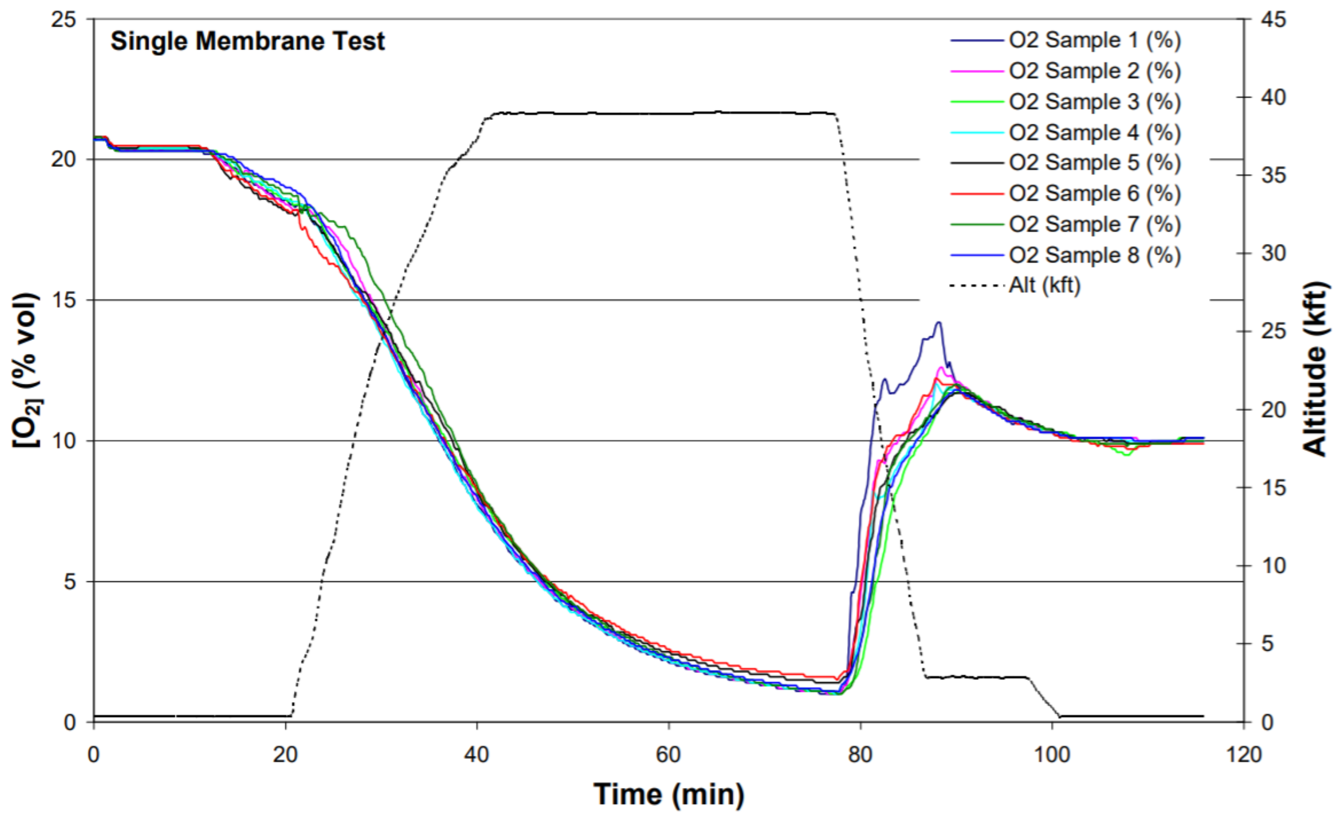
Figure 6.
Inerting flight test tank oxygen concentration measurements for an empty tank in different positions (samples). Note that the increase in oxygen concentration at min is due to air ingestion in the fuel tanks during the descent phase (source [14]).
The diffusion coefficients between the interacting substances can be considered as constant during the flight evolution:
which corresponds to a flight profile at a total environmental (static and dynamic) temperature of °C. Note that the diffusion coefficients can be determined at any temperature [23]:
where and are the diffusion coefficients at temperatures and expressed in K.
The calibration exercise to assess the parameters requires the measurement of the nitrogen (N) or the oxygen concentration (). Aiming to calibrate on and for the sake of simplicity, the air is assumed to be an homogeneous mixture formed of nitrogen and oxygen. The flight test data measure the oxygen concentration in the centre tank of an Airbus A320 [14]. Figure 6 considers the case of an empty tank and one nitrogen gas generator acting (single membrane).
An empty tank is defined as that with low level of fuel and high level of fuel vapours. It is usual that the inerting system is constituted by several inert gas generators or air separation modules (ASM). This is important to increase the inerting capacity and reduce risks. An empty tank has a higher level of oxygen that shall be replaced by nitrogen to provide an inert condition. In addition, a test case with a single acting ASM is considered, which means that only one ASM is available to filter the nitrogen and remove the oxygen. This is conservative and leads to the most demanding configuration for the single inerting ASM which, in turn, will lead to provide higher lead times to get the inert condition.
The flight test data compiled in Figure 6 are interpreted over homogeneous mean oxygen values to define the parameters n and m. Hence, the flat problem P is:
For each time step, the time derivatives and are determined. For this purpose, it is considered that the substance concentrations are expressed between the interval and the time is expressed in minutes. Such time derivatives are obtained for different discrete times and represented versus the concentration of each substance. Afterwards, the optimal curve fitting is determined as
Therefore, . The same process for provides:
Then, . The parameters obtained, based on flight test data, are indeed between , as initially appointed.
Then, the forced convective parameter a is obtained. For this purpose, the basic continuity equation is used:
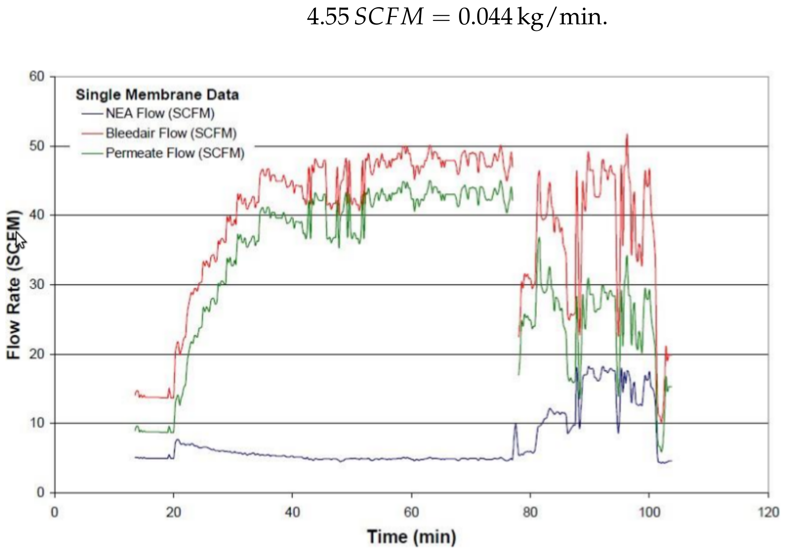
where G is the inerted gas flow, rich in nitrogen, and D is the air density within the fuel tank, mainly constituted of nitrogen in stabilized flight. Note that the nitrogen flow is kept stable during the flight and increases during the descend phase. For the calibration exercise, it is considered the flight cruising phase (at min), in which the nitrogen flow value is given by Figure 7:
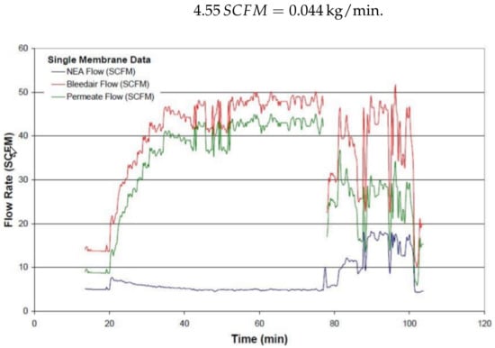
Figure 7.
Involved mass flow for the single membrane (only one inerting generator working) flight test. The cruise phase (stabilized flight) is obtained at min and the descent phase starts at min (source [14]).
The gas density (D) is obtained based on the predominant nitrogen and remaining oxygen. It is considered an average value of of nitrogen and of oxygen during the cruise phase (stabilized flight):
The A320 centre fuel tank is almost of rectangular shape with a mean height of 1.5 m and a mean wide of 6 m:
Then, a can be determined as per (33) m/min.
After calibration, the problem P is summarized as
Once the model parameters have been obtained, TW solutions are provided for the initial concentrations given by the level of nitrogen and oxygen in the standard atmosphere:
The TW solutions are formed of a front and a tip. The front carries the information transition in the media from one state to the other. This kind of behaviour exhibited can be applied to the propagation of the nitrogen gas within the fuel tank. The nitrogen TW constitutes a propagating front that shifts the tank ullage concentration by reducing the oxygen and increasing the nitrogen.
Note that there exist stationary solutions given by the initial conditions and the asymptotic approximation. Such asymptotic solutions are provided by the levels of concentration admitted by the particular technology employed (see [10] for a description). For this purpose, it is considered that min (according to Figure 6 and previously to starting the descent phase) is sufficiently large time for the stationary solutions:
The problem analysed in the travelling wave domain, adopts the form:
where the parameters and a are given in (37). In this case, a corrected speed is introduced to account for the advection term. Then:
To determine the TW propagation speed, we first consider that the TW front and tip move with corrected speed , so that when the variable , the wave has propagated along the whole domain:
Once the TW has finished the propagation along the tank, the inerted level corresponding to is reached. At min, the TW has reached all tank areas to provide the lowest value, measured in flight, for the oxygen concentration. In addition, x is a typical tank dimension obtained as the geometric mean of the tank shape:
After assessing the TW speed, the model (40) is solved with the function bvp4c in Matlab, as shown in Section 3.2. The results, in the TW variable , are compiled in Figure 8.
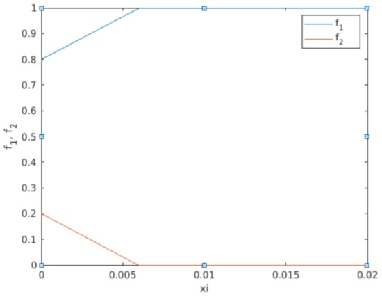
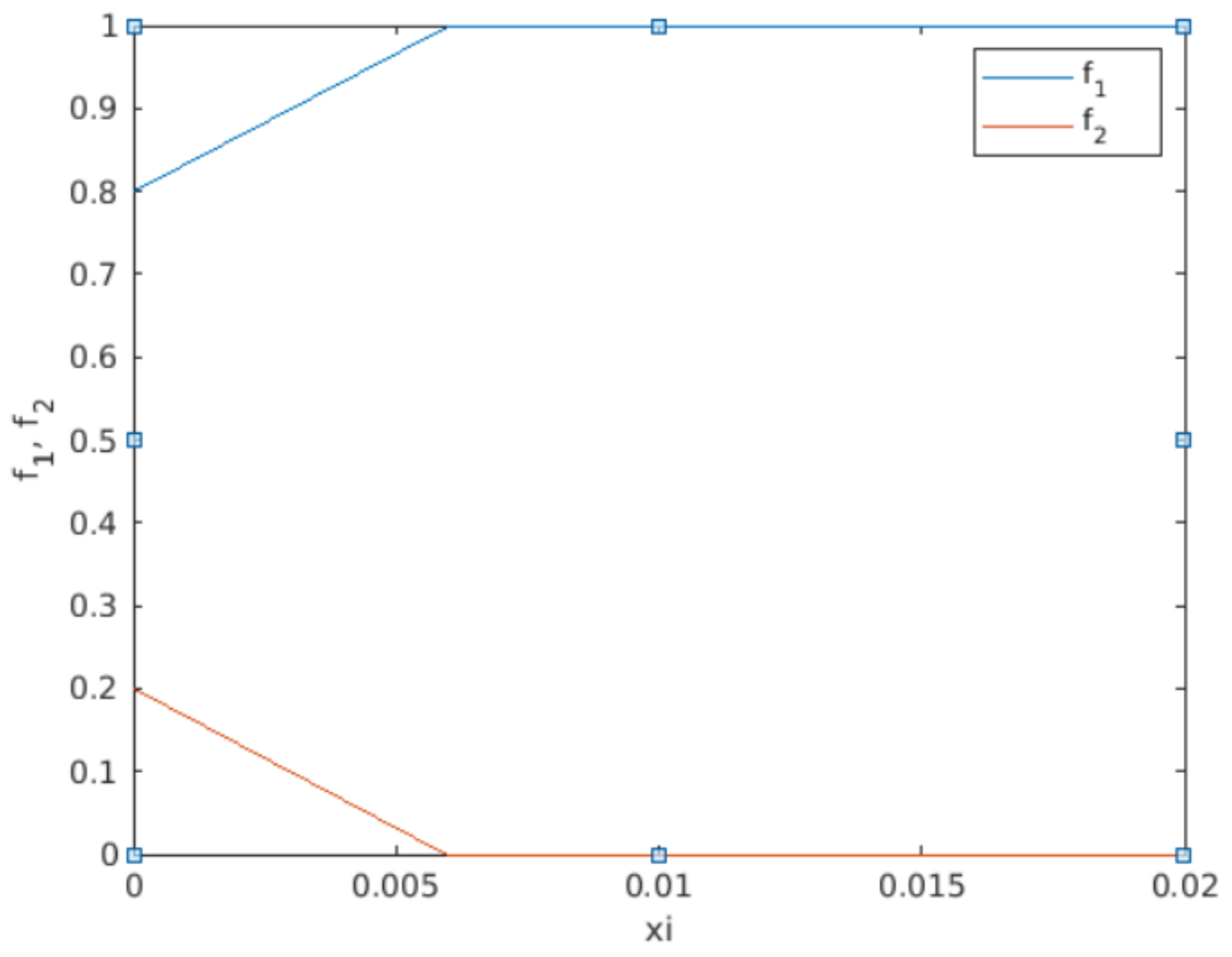
Figure 8.
Travelling wave solutions. The blue solution represents the evolution of the nitrogen within the tank evolving from ( in volume) up to filling the whole tank 1 (). The red solution represents the oxygen density that evolves from ( in volume) down to zero. Note that the horizontal axis represents the variable , while and .
The time required to reach a certain level of nitrogen N that ensures an inerted condition is then obtained. As an example, a concentration of of oxygen in a fuel tank is sufficient to get the inert status [24]. A value of corresponds to the following value of (Figure 8):
To determine the time to inert, we consider that the advection term acts physically in the same direction as the TW-speed . This assumption is realistic as the forced convection drives the nitrogen to all tank areas where the gas is free to flow. Nonetheless, once the nitrogen is in complicated tank shapes, it moves by diffusion only. Hence, the forced convection (a) and the diffusive TW () are summative terms that act to reach the inert condition in all tank areas (both free paths and difficult geometries). Thus, the time to obtain the inerted configuration under similar operational conditions compared to the A320 aircraft is:
Globally, at min, the tank will reach a value of of oxygen in all areas. This value is overly pessimistic compared to the value provided in Figure 6, in which the value of of oxygen is obtained at min. Nonetheless, the values of oxygen in Figure 6 are only provided for different locations where the oxygen sensors are placed. Therefore, the modelled value of min, shall be seen as an approach in which the diffusion acts as per the travelling wave front and tip to cover the whole domain.
It is particularly relevant to observe that the scale for the tank dimension ( m) is much higher than the scale of the TW spatial variable . This fact can be explained in view of the TW features. The front and the tip represent the diffusion acting along the wave so that represents a dimension of the wave interface where the front and the tip are confined.
4. Conclusions
The problem proposed with a coupled system of reaction diffusion equations to model an aircraft fuel tank inerting process has been discussed with a mathematical approach stressing aspects related with the existence, uniqueness and behaviour of solutions in the travelling wave domain. The application exercise to a centre fuel tank on an Airbus A320 set the evidence for the use of the problem to model inerting processes in aircraft. The information provided permitted the mathematical representation of the oxygen and nitrogen concentrations and enabled our understanding of the dynamic of the process based on a parabolic coupled system of equations.
In addition, finite values for the model parameters and a have been shown to exist, and furthermore, the combination of such values has been shown to provide global solutions in the TW frame. Eventually, the model has been shown to provide an answer to a basic question asked by the engineering and physical application, i.e., the global time required to ensure a fuel tank is safe (inerted) to prevent explosion due to the presence of oxygen in the tank ullage.
Funding
This research received no external funding.
Acknowledgments
The study has been founded by the Research Directorate at Universidad Francisco de Vitoria.
Conflicts of Interest
The author declares that there is no conflict of interest.
References
- Fisher, R.A. The advance of advantageous genes. Ann. Eugen. 1937, 7, 355–369. [Google Scholar] [CrossRef] [Green Version]
- Kolmogorov, A.N.; Petrovskii, I.G.; Piskunov, N.S. Study of the diffusion equation with growth of the quantity of matter and its application to a biological problem. Dyn. Curved Front. 1937, 1937, 105–130. [Google Scholar]
- Aronson, D. Density-dependent interaction-diffusion systems. In Dynamics and Modelling of Reactive Systems; Academic Press: New York, NY, USA, 1980. [Google Scholar]
- Aronson, D.; Weinberger, H. Nonlinear diffusion in population genetics, combustion and nerve propagation. In Partial Differential Equations and Related Topic; Springer: New York, NY, USA, 1975; pp. 5–49. [Google Scholar]
- Aronson, D.; Weinberger, H. Multidimensional nonlinear diffusion arising in population genetics. Adv. Math. 1978, 30, 33–76. [Google Scholar] [CrossRef] [Green Version]
- Cangiani, A.; Georgoulis, E.H.; Morozov, A.; Sutton, O.J. Revealing new dynamical patterns in a reaction–diffusion model with cyclic competition via a novel computational framework. Proc. R. Soc. 2018, 474. [Google Scholar] [CrossRef]
- Volpert, V.; Petrovskii, S. Reaction-diffusion waves in biology. Phys. Life 2009, 6, 267–310. [Google Scholar] [CrossRef]
- Barenblatt, G.I.; Zeldovich, Y.B. On stability of flame propagation. Prikl. Mat. Mekh. 1957, 21, 856–859. (In Russian) [Google Scholar]
- Federal Aviation Administration. Advisory Circular Ref. 25.981-1C. Fuel Tank Ignition Source Prevention Guidelines; Federal Aviation Administration: Washington, DC, USA, 2008.
- SAE International. Aircraft Fuel Tank Inerting Systems; SAE Ref ARP6078; SAE International: Warrendale, PA, USA, 2012. [Google Scholar]
- Cavage, W.M.; Bowman, T. Modeling in flight inert gas distribution in a 747 center wing fuel tank. In Proceedings of the 35th AIAA Fluid Dynamics Conference and Exhibit, Toronto, ON, Canada, 6–9 June 2005. [Google Scholar]
- Burns, M.; Cavage, W.M. Inerting of a Vented Aircraft Fuel Tank Test Article with Nitrogen Enriched Air; Report for the Federal Aviation Administration, Report No. DOT/FAA/AR-01/6; Federal Aviation Administration: Washington, DC, USA, 2001.
- Ghadirian, E.; Brown, J.; Wahiduzzaman, S. A Quasy-Steady Diffusion Based Model for Design and Analysis of Fuel Tank Evaporate Emissions; SAE Technical Paper Ref. 2019-01-0947; SAE International: Warrendale, PA, USA, 2019. [Google Scholar]
- Burns, M.; Cavage, W.; Hill, R.; Morrison, R. Flight-Testing of the FAA Onboard Inert Gas Generation System on an Airbus A320. DOT/FAA/AR-03/58; U.S. Department of Transportation Federal Aviation Administration: Washington, DC, USA, 2004.
- Feng, S.; Li, C.; Peng, X.; Wen, T.; Yan, Y.; Jiang, R.; Liu, W. Oxygen concentration variation in ullage influenced by dissolved oxygen evolution. Chin. J. Aeronaut. 2020. [Google Scholar] [CrossRef]
- Banerjee, R.A. A numerical study of combined heat and mass transfer in an inclined channel using the VOF multiphase model. Numer. Heat Transf. Part A Appl. 2007, 52, 163–183. [Google Scholar] [CrossRef]
- Karpinska, A.M.; Bridgeman, J. CFD-aided modelling of activated sludge systems—A critical review. Water Res. 2016, 88, 861–879. [Google Scholar] [CrossRef] [PubMed] [Green Version]
- Kiselev, V.G. Fundamentals of diffusion MRI (Magnetic Resonance Imaging) Physics. NMR Biomed. 2017, 30, 3602. [Google Scholar] [CrossRef] [PubMed]
- Bhatti, M.; Zeeshan, A.; Ellahi, R.; Anwar Bég, O.; Kadir, A. Effects of coagulation on the two-phase peristaltic pumping of magnetized prandtl biofluid through an endoscopic annular geometry containing a porous medium. Chin. J. Phys. 2019, 58, 222–223. [Google Scholar] [CrossRef]
- Ellahi, R.; Hussain, F.; Ishtiaq, F.; Hussain, A. Peristaltic transport of Jeffrey fluid in a rectangular duct through a porous medium under the effect of partial slip: An application to upgrade industrial sieves/filters. Pramana J. Phys. 2019, 93, 34. [Google Scholar] [CrossRef]
- Pao, C.V. Nonlinear Parabolic and Elliptic Equations; Springer: Berlin/Heidelberg, Germany, 1992. [Google Scholar]
- Enright, H.; Muir, P.H. A Runge-Kutta Type Boundary Value ODE Solver with Defect Control; Teh. Rep. 267/93; University of Toronto, Dept. of Computer Sciences: Toronto, ON, Canada, 1993. [Google Scholar]
- Bird, R.B.; Stewart, W.E.; Lightfoot, E.N. Transport Phenomena; John Wiley & Sons: Hoboken, NJ, USA, 1960; p. 780. [Google Scholar]
- Kuchta, J.M. Oxygen Dilution Requirements for Inerting Aircraft Fuel Tanks; Bureau of Mines Safety Research Center: Washington, DC, USA, 1970; pp. 85–115. [Google Scholar]
Publisher’s Note: MDPI stays neutral with regard to jurisdictional claims in published maps and institutional affiliations. |
© 2021 by the author. Licensee MDPI, Basel, Switzerland. This article is an open access article distributed under the terms and conditions of the Creative Commons Attribution (CC BY) license (https://creativecommons.org/licenses/by/4.0/).