Article

Thrust Augmentation of Micro-Resistojets by Steady Micro-Jet Blowing into Planar Micro-Nozzle

by
Donato Fontanarosa
,
Maria Grazia De Giorgi
* and
Antonio Ficarella
Research Center for Energy and Environment (UNISALENTO-DII-CREA), Department of Engineering for Innovation, University of Salento, Via per Monteroni, I-73100 Lecce, Italy
*
Author to whom correspondence should be addressed.
Appl. Sci. 2021, 11(13), 5821; https://doi.org/10.3390/app11135821
Submission received: 22 April 2021 / Revised: 13 June 2021 / Accepted: 15 June 2021 / Published: 23 June 2021
(This article belongs to the Special Issue Micro Power Technologies for Air and Space Vehicles)

Abstract

:

Featured Application

Secondary micro-propulsion systems for small satellites.

Abstract

The present work investigates the impact of steady micro-jet blowing on the performance of a planar micro-nozzle designed for both liquid micro-thrusters and nitrogen cold-gas micro-resistojets. Two micro-injectors have been placed into the divergent region along the sidewalls, injecting a secondary flow of propellant perpendicularly to the wall where they have been located. The micro-jet actuator configuration is characterized by the dimensionless momentum coefficient cμ. The best performance improvement is retrieved at the maximum cμ for both water vapor ( Δ % T , j e t = +22.6% and Δ % I s p , T j e t = +2.9% at cμ = 0.168) and nitrogen gaseous flows ( Δ % T , j e t = +36.1% and Δ % I s p , T j e t = +9.1% at cμ = 0.297). The fields of the Mach number and the Schlieren computations, in combination with the streamline visualization, reveal the formation of two vortical structures in the proximity of secondary jets, which energize the core flow and enhance the expansion process downstream secondary jets. The compressible momentum thickness along the width-wise direction θxy in presence of secondary injection reduces as a function of cμ. In particular, it becomes smaller than the one computed for the baseline configuration at cμ > 0.1, decreasing up to about and -57% for the water vapor flow at cμ = 0.168, and -64% for the nitrogen gaseous flow at cμ = 0.297.

1. Introduction

The micro-satellite is a device of great interest in space research, because it is cost-effective. In this field, the micro-thrusters present optimal characteristics for attitude control, orbit maintenance, and station maintenance, thanks a precise control of operating conditions [1]. In this regard, an onboard secondary propulsion system should be installed, which is able to provide small thrust forces from a few micro-newtons up to some milli-newton and high specific impulse, still satisfying the mass, volume, and power consumption constraints [2].
Different concepts of MEMS-based micro-propulsion systems, or micro-thrusters, have been developed to be implemented in small satellites [3,4]: thanks to the reduced system complexity related to the simplicity of the working principle, micro-resistojets represent a very interesting choice. Among them, cold gas micro-thrusters (CGs) operate with gaseous propellants; when operating with liquid propellants, micro-resistojets are usually referred to as vaporizing liquid micro-thrusters (VLMs) [5,6]. Increasing interest of the industrial and scientific communities on VLMs is due to their simplicity and compactness and the possibility to use water as green propellant. The use of water matches all requirements in terms of propulsive performance (associated mainly to thrust and specific impulse), system density (associated to mass and size), and safety (associated to flammability, instability, and health hazard), as discussed in [7].
However, by considering the global performance of micro-resistojets, the micro-nozzle overall efficiency is strongly affected by the entity of the viscous effects [8,9]. These last ones are influenced by the degree of gas rarefaction, since it determines the mechanisms of interaction between gas–gas molecules and solid wall–gas molecules. In general, in micro-nozzles, the continuum assumption and the no slip condition at walls are violated, and two different regimes could establish based on the entity of the Knudsen number Kn [10], which is defined as the ratio between the mean free molecular path and the characteristic length as follows:
K n = Λ L = k π 2 M R e ,
where Λ is the mean free path of the gas molecule, L is the characteristic length, and M and Re are the Mach and the Reynolds numbers, respectively. Consequently, when 0.01 < Kn < 0.1 the slip flow regime occurs, while the transitional flow regime occurs if 0.1 < Kn < 10. In cases involving the first regime, the Navier–Stokes (NS) equations are still valid for numerical modeling, even in combination with partial slip models at walls [11].
In this regard, in [12], the optimization of the divergence half-angle of conical micro-nozzle was performed in order to increase the thrust; it was shown that the optimum angle little depends on the given nozzle length, and it is almost independent of gas species and heat loss. In [13], heating the convergent–divergent sidewall was studied as a method to improve the thrust level and specific impulse. However, a degradation of Mach number and velocity and an increase in the thickness of the sub-sonic boundary layer were found. The performance of the micro-nozzle is also influenced by surface roughness on outlet flow velocity [14]. In [15], it was shown that pressure disturbances in under-expanded micro-nozzle flow can propagate upstream due to the development of the boundary layer causing the flow blockage. In [16], surface discontinuities on the divergent contour of the micro-nozzle were investigated in order to assess the sensitivity of the pressure, skin friction, and heat transfer coefficients to these discontinuities as well as their impact on the specific impulse. The growth of the sub-sonic boundary layer reduced the thrust efficiency due to the viscous losses and the reduction of the actual cross section at the nozzle exit [17]. Later, in [18], it was shown that the Mach number near the downstream position of the micro-nozzle’s throat is lower than that in the conventional nozzle and that the position of the sonic point moves away from the throat toward the outlet if the size of the nozzle decreases. This specific behavior is ascribed to the higher viscous dissipation in micro-nozzles with respect to the macro-scale flow nozzles. More recently, viscous losses on boundary layer of rarefied gas flows inside micro-nozzles in the slip regime condition could lead to a reduction of the nozzle performance of about the 95%, as shown in [9].
In large-scale nozzles, the use of secondary injection as active fluidic flow control strategy has been investigated since the 1960s using both gaseous [19] and liquid [20] secondary jets to extend the propulsive performance of different kinds of nozzles, such as single expansion ramp nozzles for scramjets [21], dual-throat nozzles [22,23], dual-bell nozzles [24], aero-spike nozzles [25], and biconical nozzles [26]. More recently, many numerical and experimental works have followed to extend the knowledge of the transition phenomena involved in the interaction between the secondary jet and the super-sonic flow expanding into the nozzle, such as [27], and to optimize the effectiveness of such active control system over a variety of parameters, for instance, injector location, number, shape, angles, cross section, and flow momentum [28,29,30,31].
Despite the large amount of literature on the use of secondary injection in large-scale nozzles, there is a lack about the implementation of steady micro-jet blowing into planar micro-nozzles for viscous losses mitigation and thrust augmentation. The present work aims to fill this knowledge gap by providing a numerical investigation of the impact of such active fluid flow control of performance of a planar tronco-conical micro-nozzle geometry applied to MEMS-based micro-resistojets operating as water VLM or nitrogen CG. The overall investigation has been conducted on the planar geometry designed by Cen and Xu [32], where the entity of viscous losses is increased due to the relatively long divergent. The analysis is based on 3D CFD computations conducted using NS with Maxwellian partial slip at walls with a tangential momentum accommodation co-efficient (TMAC) equal to 0.80. The estimation of the global performance of the micro-nozzle was performed in terms of percent variation of thrust force, specific impulse, and mass flow rate, coupled with the calculation of the boundary layer thicknesses at the micro-nozzle exit. Furthermore, a qualitative description of the flow behavior based on the Mach number contour plot highlighted the differences among the investigated cases. The paper is structured as follows: Section 2 describes the micro-nozzle geometry and the active flow control configuration; Section 3 provides the description of the numerical setup and the overall investigation logic and methodology; Section 4 presents and discusses the results underlining the most interesting findings; and finally, Section 5 is devoted to conclusions and final remarks.

2. Micro-Nozzle and Active Flow Control Configuration Using Secondary Injection

2.1. Micro-Nozzle Geometry

The micro-nozzle planar geometry investigated in the present work was the same of the VLM developed by Cen and Xu [32]. It consists of a rectangular plenum upstream; followed by a heating chamber composed of nine parallel micro-channels of 8 × 10⁻⁵ m width; and a convergent–divergent planar nozzle having a throat width of 1.5 × 10⁻⁴ m, inlet cross section width of 1.07 × 10⁻³ m, outlet cross section width of 1.76 × 10⁻³ m, and convergent and divergent angles of 45° and 15°, respectively (see Table 1). Furthermore, as shown in Figure 1, a radius of curvature at the throat section equal 7.5 × 10⁻⁵ m was also considered in combination with a mixing region of 1.8 × 10⁻⁴ m length before the entrance into the convergent region. Finally, the nozzle depth is 1.2 × 10⁻⁴ m.

2.2. Secondary Injection Configuration

Concerning the configuration of the secondary injection system, two micro-jets, from here on denoted as “jet 1” and “jet 2”, have been placed along the sidewalls of the divergent region, with jet centerlines located at an axial distance from the throat section, equal to xjet,1 = 1.73 × 10⁻³ m and xjet,2 = 2.475 × 10⁻³ m, as shown in Figure 2. As summarized in Table 2, the micro-jets have been injected from micro-channels owning exit cross section of rectangular shape, and dimensions of 40 μm × 120 μm and 50 μm × 120 μm, respectively for jet 1 and jet 2.
A fixed velocity boundary condition reproduced the behavior of the secondary micro-jet blowing, i.e., U j e t = U j e t n ^ j e t , where Ujet is the jet velocity magnitude and n ^ j e t = (cos(αjet), sin(αjet)) is the jet direction with respect to the micro-nozzle sidewall plane, as shown in Figure 2. The micro-jet blowing has been activated once the steady-state conditions without actuation has been established in the micro-nozzle, which also refers to the baseline configuration, from here on denoted also by the subscript 0.
Furthermore, each secondary jet configuration was defined by the momentum co-efficient cμ, which is the ratio between the secondary jet momentum and the one owned by the main flow before actuation, as follows:
c μ = m ˙ j e t U j e t m ˙ 0   U 0 , xjet
where U0,xjet is the axial velocity of the core flow at x = xjet, while m ˙ 0 and m ˙ j e t represent the main flow and the secondary jet mass flow rates, respectively. It is worth observing that Equation (2) provides a measure of the relative intensity of the jet with respect to the core flow.
In the case of two jets, cμ,tot will be the sum of cμ,jet1 and cμ,jet2.

2.3. Micro-Nozzle Performance Estimation

The performance of the micro-nozzle have been analyzed in terms of thrust force T and specific impulse Isp as follows:
T = T j e t + T p r e s s = m ˙ t o t U e x i t + ( p e x i t p a m b ) A e x i t = m ˙ t o t U e f f
I s p = T ( m ˙ t o t   g 0 )      
where U is the flow velocity, p is the static pressure, and g0 ≈ 9.81 m/s is the gravitational acceleration at sea level. In regards to the subscripts, jet and press refer to the jet thrust and the pressure thrust, and eff denotes the effective velocity at the micro-nozzle exit, while the subscripts exit and amb respectively refer to the exit and ambient discharge conditions. Furthermore, m ˙ t o t is the total mass flow rate exiting from the micro-nozzle, defined as follows:
m ˙ t o t = A e x i t ρ   ( U × n ^ A )   d A = m ˙ 0 + m ˙ j e t , 1 + m ˙ j e t , 2
The thrust co-efficient cT has been estimated to take account the feeding pressure as an indicator of the cost supported to ensure the operating condition, as follows:
c T = T ( p i n l e t A * )
where pinlet is the total pressure at the micro-nozzle inlet, and A* is the throat section. It is worth observing that c T relates the thrust force to the cost of feeding the corresponding mass flow rate. Thus, if the mass flow rate of the core flow increases, the thrust will increase, too. However, secondary injection is provided at the same feeding pressure of the core flow by exploiting the pressure drop between the feeding pressure in the propellant storage upstream and the pressure of the expanding flow into the micro-nozzle divergent without any additional cost of feeding.
The efficiency of the micro-jet blowing has been analyzed by comparing the micro-nozzle performance of each actuated condition, denoted by the subscript i, to the ones resulting from the steady-state solution without actuation, denoted with the subscript 0. The last one also corresponds to the solution of the baseline test case. It is worth observing that the jet thrust contribution is the most relevant one, since it represents a quality term of the expansion process into the divergent section, which leads to the actual thrust force acting on the micro-thruster. On the other hand, the pressure thrust is a thrust loss term, since it increased as the quality of the expansion process reduced. Consequently, the performance analysis has been based on the estimation of the percent variation of the thrust co-efficient Δ % c T , jet thrust Δ % T , j e t , specific impulse related to the jet thrust Δ % I s p , j e t , and mass flow rate Δ % m ˙ for each actuated condition i as follows:
Δ % c T = ( c T , i c T , 0 ) c T , 0 100
Δ % T , j e t = ( T j e t , i T jet , 0 ) T jet , 0 100
Δ % I s p , j e t = ( I s p ,   j e t , i I s p ,   j e t , 0 ) I s p , j e t , 0   100
Δ % m ˙ = ( m ˙ t o t , i m ˙ t o t , 0 ) m ˙ t o t , 0   100
The analysis has been extended by the computation of the displacement and the momentum thicknesses at the exit section, δ *   and θ , respectively, as follows:
δ * = 0 ( 1 ρ U x ( ρ U x ) ) d y
θ = 0 ρ U x ( ρ U x ) ( 1 U x U x , ) d y
where x and y denote the parallel and normal directions to the solid wall, and the subscript refers to the undisturbed flow condition.

3. Numerical Setup and Methodology

3.1. Numerical Approach and Setup

The numerical simulations of the gas flow through the micro-nozzle were performed by using the open source CFD toolbox OpenFOAM© Version 3.0.1, based on a Finite Volume formulation. The density-based solver rhoCentralFoam [34] was used for computations. In particular, the compressible Navier–Stokes (NS) equations were solved in combination with the laminar flow approximation in reference to the turbulence modeling. This choice resulted from computations that revealed the Reynolds number of the steam flow along the mid axis of the nozzle ranging from about 3150 at the throat section up to about 600 at the exit section. Furthermore, the gas rarefaction effects have been considered by setting a partial slip boundary condition at walls with tangential momentum accommodation co-efficient σTMAC equal to 0.80. The last settings result from previous CFD computations [4], which have demonstrated that the maximum Knudsen number into the divergent is strictly below 0.1.
Concerning numerical schemes, the central upwind scheme of Kurganov and Tadmor [35] was used for the flux terms and the Total Variation Diminishing (TVD) van Leer limiter [36] for interpolation. Moreover, the Gauss linear scheme was used for the divergence, the gradient, and the Laplacian operators. Time derivatives were computed with the first order, bounded and implicit Euler scheme. The time step was determined based on a maximum Courant number Comax of 0.2. In particular, the pre-conditioned conjugate gradient/diagonal incomplete Cholesky scheme with a residual tolerance of 1 × 10⁻⁸ was used to solve the viscous governing equations, while the inviscid equations of momentum and energy were explicitly solved by means of a Gauss–Siedel Smooth solver with a residual tolerance of 1 × 10⁻¹⁰. The numerical stability during transients was ensured by splitting each simulated temporal window into three temporal intervals, i.e., [0–0.5 × 10⁻⁴] s, [0.5 × 10⁻⁴–1 × 10⁻⁴] s, and [1 × 10⁻⁴–3 × 10⁻⁴] s, and increasing the mass flow rate at the beginning of each step. The establishment of the steady state regime was ensured by monitoring the Mach number at mid-point of the nozzle exit. The Peng Robinson model [37] was used as equation of state for both water vapor and gas nitrogen, which allowed for better reproduction of the compressibility effects.

3.2. Grid Sensitivity Study

In the present work, the definition of the proper refinement level resulted from a grid independence study (GIS) based on the analysis of water vapor flow at m ˙ = 5 mg/s, Tinlet = 505.58 K and pout = 500 Pa. It was split into two steps:
  • a 2D GIS in the planar mid-section of the micro-nozzle, i.e., the plane (0,x,y) in Figure 3;
  • a 3D GIS to define the proper refinement level along the micro-nozzle depth direction (the z-direction in Figure 3).
In both studies, the discretization error between two consecutive refinement levels was estimated by computing the grid convergence index (GCI), as suggested by [38].
In particular, the 2D GIS was successfully performed and discussed in the previous work [4], to which the authors refer for further details. The summary of the 2D GIS is reported in Table 3: the 2D GIS led to the choice of the intermediate refinement level corresponding to an error of about GCI12 = 0.35%.
Once we defined the refinement level in the plane (0,x,y), the 3D mesh was built by extrusion along the micro-nozzle depth direction, i.e., the z-axis in Figure 3. Therefore, the 3D GIS was performed to define the proper refinement level into the micro-nozzle along depth-wise direction (z-axis in Figure 3), which ensured the best trade-off between accuracy and computational cost.
In this regard, the 3D computational domain composed of the micro-nozzle geometry and an outer discharge domain extending 5Wexit upward, 10Wexit downstream, and 50Hn sideways, where Wexit refers to the width of the micro-nozzle exit, and Hn is the micro-nozzle depth. The 3D refinement of the mesh involved the micro-nozzle region and the thin region of the outer domain downstream of the micro-nozzle exit invested by the plume. In particular, three uniform grid steps have been considered in the depth-wise direction, i.e., 20 μm, 15 μm, and 10 μm, which corresponded to overall 3D mesh sizes of 493,520 cells (coarse mesh level), 516,360 cells (intermediate mesh level), and 607,720 cells (fine mesh level). Due to the small thickness of the computational domain affected by the mesh refinement, the overall mesh sizes do not provide indication of the refinement level. Therefore, the grid spacing was defined by the grid steps along the z-axis direction, leading to spacing factors of 1, 1.5, and 2 from fine to coarse refinement, as summarized in Table 4.
The compressible momentum thickness at the exit section of the sidewall in the symmetry plane (0,x,y) was used as a grid convergence index (CGI) parameter, allowing us to estimate the discretization errors. Both fine-to-intermediate error GCI12 and intermediate-to-coarse refinement error GCI23 were computed, and the minimum among them was assumed the mesh refinement error. As reported in Table 4, the refinement error was about GCI23 = 5.26% during the coarse-to-intermediate refinement step, and it decreased to GCI12 = 0.67% when the mesh was refined from the intermediate level to the fine one. Consequently, the intermediate mesh was chosen for this study, thanks to the best trade-off between accuracy and computational cost, as confirmed by computational time per 0.0002 s simulated time.

3.3. Validation, Boundary Conditions, and Test Matrix

The present numerical methodology has been previously validated in [4]. Without going into details of the previous work, a numerical methodology was proposed to predict the performance of VLMs, which combined a 1D model with 3D CFD computations of the micro-nozzle flow. Using the experimental data provided in [32], the methodology allowed us to estimate the flow conditions at the micro-nozzle entrance for a given mass flow rate and wall temperature, which defined the boundary conditions in the 3D CFD computations performed using the same numerical approach and setup previously described in Section 3.1. In particular, at inlet conditions of 505.58 K temperature, 5 × 10⁻⁶ kg/s mass flow rate, and 500 backward discharge pressure, 3D CFD simulations predicted a thrust force of 4.72 mN in comparison with 5.20 mN measured in experiments, with an error of about 9%. The estimation of severe viscous losses gave suggestion for the present work, with the attempt to mitigate viscous losses by means of steady micro-jet blowing into the micro-nozzle.
Consequently, the same reference operating condition has been used, i.e., a water vapor flow at inlet temperature of 505.58 K, a mass flow rate of 5 × 10⁻⁶ kg/s, and a backward discharge pressure of 500 Pa, which defined the baseline configuration. Furthermore, the water vapor flow, resulting from the operation in VLM mode, has been compared to the nitrogen gaseous flow entering the micro-nozzle at 293 K and a mass flow rate of 5 × 10⁻⁶ kg/s. in relation to operation in CG mode.
The operating condition of the secondary injection is defined by the injection angle αjet, with respect to the micro-nozzle axis, the momentum co-efficient cμ, and the number of micro-jets, i.e., single jet mode or dual jet mode. In the present study, the injection of the secondary flow was always set perpendicular to the jet cross section plane, i.e., αjet = 75°. Instead, the overall analysis was conducted by varying the jet velocity magnitude Ujet at 150 m/s, 300 m/s, and 600 m/s, corresponding to different levels of cμ.
At first, the water vapor flow was investigated on a narrow range of operating conditions and micro-jet blowing configurations with sonic injection at jet 1 and sub-sonic injection at jet 2, as reported in Table 5. Hence, the analysis was extended to the nitrogen gas flow at same mass flow rate of the baseline configuration without secondary injection and similar Reynolds number at the throat section. With the aim to provide a more accurate insight of the impact of micro-jet blowing, the analysis has been extended to a wider range of actuation conditions, as summarized in Table 6. In particular, the Mach number of the jet 1 varied from 0.43 (sub-sonic injection) to 0.86 (transonic injection) up to 1.71 (super-sonic injection). Instead, the Mach number of the jet 2 ranged from 0.43 to 0.87. Two additional test cases have been also considered:
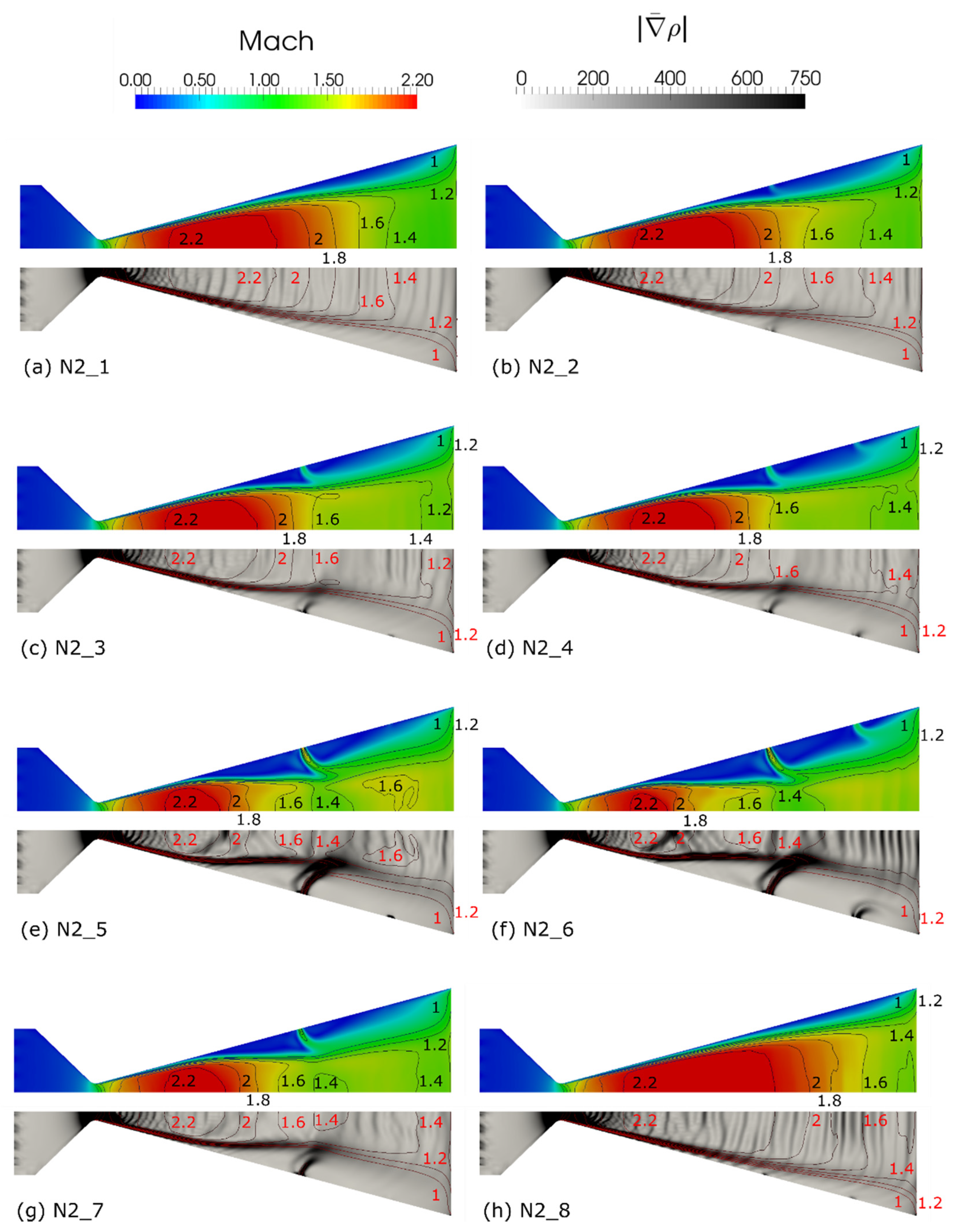
  • test case N2_7: the bypassed jet 1 activation at Mjet1 = 1.31 flow with overall mass flow rate conservation.
  • test case N2_8: configuration without secondary injection at the same mass flow rate of test case N2_6.
It is worth observing that the total mass flow rate was preserved for actuated test cases H2O_4 and N2_7 by supposing the presence of bypass micro-valves upstream the micro-nozzle, which splits the upstream mass flow rate into a core flow entering the micro-nozzle and a secondary flow directed toward the micro-jet blowing sub-system.

4. Results and Discussion

The use of secondary injection has two main purposes, namely thrust augmentation by mass addition and thrust augmentation by viscous loss reduction and flow expansion enhancement. Concerning the latter, the boundary layer growth at walls causes the establishment of the viscous choking into the divergent section and severely inhibits the super-sonic expansion of the flow, which mainly occurs into the exhaust plume downstream of the micro-nozzle exit, as confirmed in the contour plots of the Mach number in Figure 4 and Figure 5, referred to as the water vapor flow and the nitrogen gaseous flow, respectively.
In the present section, the impact of secondary injection on the super-sonic expansion of the flow into the micro-nozzle has been evaluated by coupling the analysis of the overall performance in terms of thrust force, specific impulse, and thrust co-efficient with the analysis of the flow expansion into the divergent region. The last one is based on the computation of the boundary layer thicknesses at the exit section and percent variation of the jet thrust and specific impulse related to the jet thrust, as specified in Section 2.3. Results and comparisons are summarized in Table 7 and Table 8 for the water vapor flow and Table 8 and Table 9 in the case of nitrogen gas flow.
Concerning the water vapor flow, the test cases H2O_2 and H2O_3 correspond to the secondary injection with increased total mass flow rate with respect to the baseline configuration without actuation: the former refers to single jet configuration with Δ % m ˙ = 12.6%, while the latter results from activation of both micro-jets with Δ % m ˙ = 19.2%. If the total thrust is considered, it rises from 4.489 mN of the baseline test case (H2O_1) to 5.140 mN and 5.449 mN for test cases H2O_2 and H2O_3, respectively. This leads to an improvement of the thrust co-efficient up to about 21.4%, from cT = 1.16 of test case H2O_1 to cT = 1.408 of the test case H2O_3. However, when considering the activation of the jet 1 at same total mass flow rate of the baseline configuration (test case H2O_4) through bypass, i.e., Δ % m ˙ = 0.0%, the feeding pressure at the micro-nozzle entrance decreases due to the reduced inlet mass flow rate. Despite the negligible variations of the total thrust and the specific impulse, this gives an improvement of cT of about 11.3%, which underlines a significant benefit in using secondary injection: the reduction of the energetic cost proportional to the feeding pressure.
If the jet thrust contribution is considered, the percent jet thrust augmentation Δ % T , j e t is equal to +15.9% for the test case H2O_2 and +22.6% for the test case H2O_3, as confirmed in Table 7. The last one is given by two different contributions, namely the percent mass flow rate variation Δ % m ˙ and the percent variation of the specific impulse Δ % I s p , j e t , which are equal to 12.6% and 3%, respectively, for test case H2O_2 and 19.2% and 2.9%, respectively, for test case H2O_3. Concerning the test case H2O_4, the increase of jet thrust is negligible (below 1%), as the total mass flow rate is not varied.
The improvement of the super-sonic expansion thanks to micro-jet blowing is confirmed in Figure 6, which compares the contour plots of the Mach number of all test cases in combination with Schlieren computations.
In general, the flow experiences a blocking effect due to the viscous growth of the boundary layer at the walls, as underlined by the isolines of the Mach number. However, in comparison with the baseline configuration (test case H2O_1 in Figure 6a), the presence of secondary injection mitigates these losses for test cases H2O_2 and H2O_3 (see Figure 6b,c), as highlighted by the elongation of the isoline M = 1.2 toward the micro-nozzle exit. This couples with an elongation of the super-sonic plume immediately after the micro-nozzle exit, which slightly moves the first Mach diamond region further downstream. Schlieren computations provide a more detailed view of the compressibility effects: the darkest structure appearing along the sidewalls in the divergent region reveals the presence of strong density gradients across the sonic line separating the super-sonic region (M > 1) to the sub-sonic region (M < 1), which start to develop close to the inner walls due to the boundary layer growth and then enlarge as the blocking of the flow occurs, coupled with the formation of the sub-sonic pocket region. Due to the viscous choking, the core flow is compressed as it moves toward the exit section; consequently, the intensity of the high-density gradient region softens. In presence of secondary injection, the shadow structure along the sonic line extends downstream, thanks to the energization of the main flow provided by micro-jets. In fact, by analyzing the 3D flow structures (see Figure 7), the formation of two vortical structures upstream and downstream of jet 1 is revealed, placed in the sub-sonic zone close to sidewalls. The intensity of these recirculating vortexes is proportional to cμ,1, inducing forces that accelerate the core flow along the axial direction (x-direction) and shrink it in the width-wise direction (y-direction), while pushing the sub-sonic flow upward toward sidewalls.
The enhancement of the flow expansion in the flow blocking region is also underlined in Figure 8a, comparing the axial profiles of the centerline velocity of all test cases. In particular, the core flow energization and compression by secondary injection allows for the mitigation of the viscous chocking occurring toward the exit section, with significant improvement downstream jet 1 at x > 0.002 m.
At the exit section, the profile of Ux on the middle plane reveals the beneficial impact of secondary injection on the expansion process. As shown in Figure 8b, it involves both the sub-sonic pocket and the super-sonic core, with a rise in Ux in both zones.
Concerning the nitrogen gas flow, results and comparison are summarized in Table 9 and Table 10.
To compare the effect of secondary injection in nitrogen-fed CGs with the water-propelled VLMs, similar mass flow rates and overall momentum co-efficients have been used. As a result, a higher improvement of the thrust co-efficient cT is retrieved when operating with gaseous nitrogen in CG mode. More specifically, the test cases N2_5 and N2_6 have exhibited the highest performance enhancement, with percent thrust co-efficient augmentation equal to +21.6% and +32.6%, respectively, and percent increment of total mass flow rate of 15.2% and 24.8%, respectively. The beneficial impact of secondary injection on the jet thrust is even greater: Δ % T , j e t = +26.0% and Δ % I s p , F j e t = +9.3% for the test case N2_5, and Δ % T , j e t = +36.1% and Δ % I s p , F j e t = +9.1% for the test case N2_6. By reducing the momentum co-efficient, the percent thrust augmentation decreases, too: at cμ = 0.0556 (test case N2_4), it is Δ % c T = +12.4, Δ % T , j e t = +14.2%, and Δ % I s p , F j e t = +3.9%, with Δ % m ˙ = +10.0%. It is worth observing that the stronger impact of secondary injection in nitrogen-fed CGs is likely due to the location of micro-jets in relation to the operating conditions. In fact, the quality of the expansion process of the nitrogen gaseous flow is higher than the one experienced by the water vapor flow, as highlighted by the contour plot of the Mach number in Figure 9a. This produces a thinner sub-sonic packet along sidewalls, which starts to form just before the location of the jet 1. Furthermore, for a given cμ, the kinetic energy of the micro-jet, and hence, the penetration length, in nitrogen-fed CG mode is higher than the one observed in water-fed VLM mode.
The enhancement of the expansion process is clearly underlined in the contour plots of the Mach number shown in Figure 9. In fact, with respect to the baseline configuration (Figure 9a), the isoline M = 1.4 moves downstream for the test case N2_2 (Figure 9b), approaching to the exit section for test cases N2_3 (Figure 9c) and N2_4 (Figure 9d). By increasing cμ (test cases N2_5 and N2_6), the flow undergoes a second expansion process with M > 1.4 at the micro-nozzle exit. The 3D representation of the flow in Figure 10 confirms that the expansion improvement is due to the formation of the recirculating vortexes just before and after the jet 1. Comparing to the water-fed cases shown in Figure 7, test cases N2_5 and N2_6 exhibit stronger and larger vortical structures, which affect the core flow more deeply up to break the expansion process in correspondence of jet 1. This allows the core flow to gain energy and expand more efficiently downstream of the jet 1.
The Schlieren images in Figure 9 show the impact of secondary injection on the density gradients. In general, in comparison with the water-fed VLM cases, a more pronounced gray is computed along the sonic line due to the smaller sub-sonic pocket and the more abrupt density change: this confirms the higher effectiveness of such flow control strategy when operating in nitrogen-fed CG mode. As expected, the most significant impact on the expanding flow is retrieved at the highest cμ (test cases N2_5 and N2_6): the jet 1 deeply penetrates the core flow, shrinking it and producing an enlargement of the sub-sonic region. Consequently, the super-sonic core flow is compressed when crossing the jet 1 region; then, it expands immediately after with suppression of the viscous choking toward the exit section.
The comparison between test cases N2_6 and N2_8 analyzes the use of secondary injection in relation to the similar increase of total mass flow rate in the core flow (i.e., Δ % m ˙ = +24.8%) without any fluidic flow control. As reported in Table 8 and Table 9, a weak difference is retrieved in percent jet augmentation: Δ % T , j e t = +36.1% in presence of micro-jet blowing (N2_6) and Δ % T , j e t = +32.8% with equivalent core mass flow rate increase (N2_8). However, the more the core mass flow rate is, the higher the feeding pressure must be and, consequently, the more the cost per unit of thrust results. In fact, p0 increases from 1.287 × 10⁵ Pa to 1.608 × 10⁵ Pa for test case N2_8, and the percent increase of the thrust co-efficient is reduced from +32.9% (test case N2_6) to Δ % c T = +2.9% (test case N2_8). Similar finding results are achieved by comparing the baseline test case N2_1 with the test case N2_7, owning active micro-jet blowing and bypassed mass flow rate ( Δ % m ˙ = 0.0%): Δ % c T = +13.3%, with Δ % T , j e t = +2.0%, and Δ % I s p , j e t = +2.8%.
Figure 11a shows the profile of the axial velocity Ux along the centerline: in presence of secondary injection, the higher cμ is, the sooner the flow slows down and compresses after the initial flow expansion, and the more it re-expands toward the exit section. This is in accordance with the 2D and 3D analysis previously discussed and shown in Figure 9 and Figure 10.
Instead, Figure 11b highlights the increase of the axial velocity Ux at the micro-nozzle exit (x = 0.00301 m) by showing the modification of Ux in the symmetry plane along the width-wise direction (y-coordinate). With respect to the baseline test case N2_1 (blue line with circles), the more cμ increases, the more the flow accelerates in both the sub-sonic boundary layer and the super-sonic fully developed flow region; consequently, the maximum expansion enhancement is observed at the highest cμ (test cases N2_5 and N2_6).
Regarding the boundary layer development at sidewalls, the momentum thickness along the width-wise direction at the exit section in the symmetry plane has been computed. As shown in Figure 12a, it reveals the existence of a cμ threshold limit equal to 0.1, above which the beneficial effect of secondary injection on the viscous layer at walls becomes relevant. When comparing the actuated cases to the baseline configuration (test case N2_1), θxy in presence of secondary injection is higher at cμ < 0.1, with maximum momentum thickness of about 30 μm exhibited by the test case N2_2 operating at cμ = 0.00858. On the other hand, at cμ > 0.1, θxy significantly drops down up to about 5 μm, retrieved by activating both micro-jets at the highest momentum co-efficient, i.e., the test case N2_6.
Concerning the secondary injection in water-propelled VLM mode (Figure 12b), similar beneficial impact of the micro-jet blowing active control is figured out: θxy decreases up to about −57% at the highest cμ = 0.168 (test case H2O_3), with steeper negative slope than the momentum thickness reduction curve retrieved for the nitrogen gaseous secondary injection (red dash-dotted line in Figure 12a).

5. Conclusions

The present work provides a numerical investigation of thrust augmentation of a planar convergent–divergent micro-nozzles by means of steady micro-jet blowing. The aim of such active flow control consists in hindering the viscous losses and suppress the chocking of the flow into the divergent section due to the growth of boundary layer thickness. The analysis of the micro-nozzle performance involved both water vapor and nitrogen gas as propellant, operating in a vaporizing liquid micro-thruster mode and cold gas micro-resistojet mode, respectively.
Concerning the active control configuration, two micro-injectors have been placed into the divergent region along the sidewalls, injecting a secondary flow of propellant perpendicularly to the wall where they have been located, i.e., at 75° of injection angle with respect to the micro-nozzle axis. The secondary injection has been supposed symmetric with respect to the micro-nozzle axis, leading to symmetric expanding flow. Each micro-jet blowing configuration has been defined by the overall momentum coefficient cμ, i.e., the sum of the ratios between the momentum of each secondary jet and the momentum of the core flow at the injection section. The impact of the micro-jet blowing on the micro-nozzle performance has been evaluated in terms of percent variation of the thrust co-efficient, the jet thrust Δ % T , j e t and the jet specific impulse Δ % I s p , j e t , and the estimation of the momentum thickness along the width-wise direction θxy at the exit section.
Results highlight that, at similar cμ,, Δ % T , j e t significantly increases when considering the secondary injection of gaseous nitrogen in comparison to the water vapor one. As revealed by the 3D contour plot of the Mach number in combination with streamlines visualization, this is due to the formation of larger vortical structures close to jet 1, which cause a stronger energization of the core flow expanding into the divergent section, and the consequent better expansion process just downstream to jet 1. The greatest performance improvement is retrieved at the maximum cμ for both water vapor and nitrogen gaseous flows. Concerning the former, it is Δ % T , j e t = +22.6 % and Δ % I s p , T j e t = + 2.9% at cμ = 0.168, while the latter exhibits Δ % T , j e t = +36.1 % and Δ % I s p , T j e t = + 9.1% at cμ = 0.297. The axial profiles of the centerline velocity and the velocity profile at the micro-nozzle exit along the width-wise direction highlight the mitigation of the viscous chocking of the core flow thanks to secondary injection, with enhanced flow expansion in both the subsonic pocket region close to walls and the supersonic core flow region. Furthermore, a relevant advantage in using micro-jet blowing has been pointed out by computing the percent variation of thrust coefficient Δ % c T . By comparing the baseline test case without secondary injection and test cases owning active micro-jet blowing with by-passed mass flow rate ( percent   total   mass   flow   rate   Δ % m ˙ = 0.0%), Δ % c T is higher than +10%, even though with negligible Δ % T , j e t and Δ % I s p , j e t . This is related to the reduction of the “cost” of micro-nozzle feeding, since the pressure at the micro-nozzle entrance decreases due to the reduced inlet mass flow rate. Finally, the relation θxy as a function of cμ, figures out the presence of a threshold level for cμ of about 0.1 above which θxy rapidly decreases with respect to the baseline configuration without micro-jet blowing, up to about and −57% for the water vapor flow at cμ = 0.168, and -64% for the nitrogen gaseous flow at cμ = 0.297.
The overall analysis has shown promising results, which suggest the need for a more detailed sensitivity study to provide a better insight of the influence of the secondary jet location, direction, and multi-jet configuration on the boundary layer effects and micro-thruster’s performance. Furthermore, the main challenges deserve further consideration in the next future, which are mainly related to the design and the manufacturing of the actuation of the micro-jet blowing system, which will include the feeding system and/or a micro-valve-based bypass system, super-sonic micro-injectors, and the electronics of an integrated control system.

Author Contributions

Conceptualization: M.G.D.G. and A.F.; methodology, M.G.D.G.; software, D.F.; validation, D.F.; formal analysis, M.G.D.G. and D.F.; investigation, M.G.D.G. and D.F.; resources, A.F. and M.G.D.G.; data curation, D.F.; writing—original draft preparation, M.G.D.G. and D.F.; writing—review and editing, M.G.D.G. and A.F.; supervision, M.G.D.G. and A.F. All authors have read and agreed to the published version of the manuscript.

Funding

This research received no external funding.

Institutional Review Board Statement

Not applicable.

Informed Consent Statement

Not applicable.

Data Availability Statement

Not applicable.

Conflicts of Interest

The authors declare no conflict of interest.

References

  1. Köhler, J.; Bejhed, J.; Kratz, H.; Bruhn, F.; Lindberg, U.; Hjort, K.; Stenmark, L. A hybrid cold gas microthruster system for spacecraft. Sens. Actuators A Phys. 2002, 97, 587–598. [Google Scholar] [CrossRef]
  2. Lemmer, K. Propulsion for cubesats. Acta Astronaut. 2017, 134, 231–243. [Google Scholar] [CrossRef]
  3. Silva, M.A.; Guerrieri, D.C.; Cervone, A.; Gill, E. A review of MEMS micropropulsion technologies for cubesats and pocket-qubes. Acta Astronaut. 2018, 143, 234–243. [Google Scholar] [CrossRef] [Green Version]
  4. De Giorgi, M.G.; Fontanarosa, D. A novel quasi-one-dimensional model for performance estimation of a Vaporizing Liquid Microthruster. Aerosp. Sci. Technol. 2019, 84, 1020–1034, ISSN 1270-9638. [Google Scholar] [CrossRef]
  5. Mueller, J.; Tang, W.; Wallace, A.; Lawton, R.; Li, W.; Bame, D.; Chakraborty, I.; Mueller, J.; Tang, W.; Wallace, A.; et al. Design, analysis and fabrication of a vaporizing liquid microthruster. In Proceedings of the 33rd Joint Propulsion Conference and Exhibit, Seattle, WA, USA, 6–9 July 1997; p. 3054. [Google Scholar]
  6. Fontanarosa, D.; De Pascali, C.; De Giorgi, M.G.; Siciliano, P.; Ficarella, A.; Francioso, L. Fabrication and embedded sensors characterization of a micromachined water-propellant vaporizing liquid microthruster. Appl. Therm. Eng. 2021, 188, 116625. [Google Scholar] [CrossRef]
  7. Guerrieri, D.C.; Silva, M.A.; Cervone, A.; Gill, E. Selection and characterization of green propellants for micro-resistojets. J. Heat Transf. 2017, 139, 102001. [Google Scholar] [CrossRef]
  8. Alexeenko, A.A.; Gimelshein, S.F.; Levin, D.A. Numerical Study of Flow Structure and Thrust Performance for 3-D Mems-Based Nozzles. In Proceedings of the 32nd AIAA Fluid Dynamics Conference and Exhibit, St. Louis, MO, USA, 24–26 June 2002. [Google Scholar]
  9. De Giorgi, M.G.; Fontanarosa, D.; Ficarella, A. Modeling viscous effects on boundary layer of rarefied gas flows inside micronozzles in the slip regime condition. Energy Procedia 2018, 148, 838–845. [Google Scholar] [CrossRef]
  10. Zhang, G.; Wang, L.; Zhang, X.; Liu, M. Continuum-based model and its validity for micro-nozzle flows. Jisuan Wuli/Chin. J. Comput. Phys. 2007, 24, 598–604. [Google Scholar]
  11. Kim, I.; Kwon, S.; Lee, J.W. Effect of unsteadiness and nozzle asymmetry on thrust of a microthruster. Nanoscale Microscale Thermophys. Eng. 2012, 16, 50–63. [Google Scholar] [CrossRef]
  12. Hameed, A.A.; Kafafy, R.; Asrar, W.; Idres, M. Improving the efficiency of micronozzle by heating sidewalls. AIP Conf. Proc. 2012, 1440, 409–417. [Google Scholar]
  13. Cai, Y.; Liu, Z.; Song, Q.; Shi, Z.; Wan, Y. Fluid mechanics of internal flow with wall friction and cutting strategies for micronozzles. Int. J. Mech. Sci. 2015, 100, 41–49. [Google Scholar] [CrossRef]
  14. Handa, T.; Matsuda, Y.; Egami, Y. Phenomena peculiar to under-expanded flows in supersonic micronozzles. Microfluidics and Nanofluidics 2016, 20, 166. [Google Scholar] [CrossRef]
  15. Sebastião, I.B.; Santos, W.F.N. Numerical simulation of heat transfer and pressure distributions in micronozzles with surface discontinuities on the divergent contour. Comput. Fluids 2014, 92, 125–137. [Google Scholar] [CrossRef]
  16. Bayt, R.L.; Breuer, K.S. Viscous Effects in Supersonic MEMS-Fabricated Micronozzles. Available online: https://www.semanticscholar.org/paper/VISCOUS-EFFECTS-IN-SUPERSONIC-MEMS-FABRICATED-Bayt-Breuer/23e1ee942a84ab62f8fedb3e65950696aaa06990 (accessed on 22 April 2021).
  17. Hao, P.F.; Ding, Y.T.; Yao, Z.H.; He, F.; Zhu, K.Q. Size effect on gas flow in micro nozzles. J. Micromech. Microeng. 2005, 15, 2069. [Google Scholar] [CrossRef]
  18. Liu, M.; Zhang, X.; Zhang, G.; Chen, Y. Study on micronozzle flow and propulsion performance using DSMC and continuum methods. Acta Mech. Sin./Lixue Xuebao 2006, 22, 409–416. [Google Scholar] [CrossRef]
  19. Neilson, J.H.; Gilchrist, A.; Lee, C.K. Side Thrust Control by Secondary Gas Injection into Rocket Nozzles. J. Mech. Eng. Sci. 1968, 10, 239–251. [Google Scholar] [CrossRef]
  20. Green, C.J.; McCullough, F. Liquid injection thrust vector control. AIAA J. 1963, 1, 573–578. [Google Scholar] [CrossRef] [Green Version]
  21. Shanmugaraj, G.; Jeyan, J.M.; Singh, V.K. Effects of secondary injection on the performance of over-expanded single expansion ramp nozzle. J. Phys. Conf. Ser. 2020, 1473, 012002. [Google Scholar] [CrossRef]
  22. Wang, Y.-S.; Xu, J.-L.; Huang, S.; Lin, Y.-C.; Jiang, J.-J. Experimental and numerical investigation of an axisymmetric divergent dual throat nozzle. Proc. Inst. Mech. Eng. Part G J. Aerosp. Eng. 2020, 234, 563–572. [Google Scholar] [CrossRef]
  23. Gu, R.; Xu, J.; Guo, S. Experimental and Numerical Investigations of a Bypass Dual Throat Nozzle. ASME. J. Eng. Gas Turbines Power 2014, 136, 084501. [Google Scholar] [CrossRef]
  24. Léger, L.; Zmijanovic, V.; Sellam, M.; Chpoun, A. Controlled flow regime transition in a dual bell nozzle by secondary radial injection. Exp. Fluids 2020, 61, 246. [Google Scholar] [CrossRef]
  25. Sieder-Katzmann, J.; Propst, M.; Stark, R.; Schneider, D.; General, S.; Tajmar, M.; Bach, C. ACTiVE–Experimental set up and first results of cold gas measurements for linear aerospike nozzles with secondary fluid injection for thrust vectoring. In Proceedings of the 8th European Conference for Aeronautics and Space Sciences EUCASS, Madrid, Spain, 1–4 July 2019. [Google Scholar] [CrossRef]
  26. Cuppoletti, D.R.; Gutmark, E.J.; Hafsteinsson, H.E.; Eriksson, L.E.; Prisell, E. Analysis of Supersonic Jet Thrust with Fluidic Injection. In Proceedings of the 52nd Aerospace Sciences Meeting, National Harbor, MD, USA, 13–17 January 2014. AIAA 2014-0523. [Google Scholar]
  27. Ferrero, A.; Martelli, E.; Nasuti, F.; Pastrone, D. Fluidic Control of Transition in a Dual-bell Nozzle. In Proceedings of the AIAA Propulsion and Energy 2020 Forum, VIRTUAL EVENT, 24–28 August 2020. AIAA 2020-3788. [Google Scholar] [CrossRef]
  28. Semlitsch, B.; Mihăescu, M.; Fuchs, L. Large Eddy Simulation of Fluidic Injection into a Supersonic Convergent-Divergent Duct. In Direct and Large-Eddy Simulation IX; Fröhlich, J., Kuerten, H., Geurts, B., Armenio, V., Eds.; ERCOFTAC Series; Springer: Cham, Switzerland, 2015; Volume 20. [Google Scholar] [CrossRef] [Green Version]
  29. Semlitsch, B.; Mihăescu, M. Fluidic Injection Scenarios for Shock Pattern Manipulation in Exhausts. AIAA J. 2018, 56, 4640–4644. [Google Scholar] [CrossRef]
  30. Semlitsch, B.; Cuppoletti, D.R.; Gutmark, E.J.; Mihăescu, M. Transforming the Shock Pattern of Supersonic Jets Using Fluidic Injection. AIAA J. 2019, 57, 1851–1861. [Google Scholar] [CrossRef] [Green Version]
  31. Zmijanovic, V.; Leger, L.; Depussay, E.; Sellam, M.; Chpoun, A. Experimental–Numerical Parametric Investigation of a Rocket Nozzle Secondary Injection Thrust Vectoring. J. Propuls. Power 2016, 32, 196–213. [Google Scholar] [CrossRef]
  32. Cen, J.; Xu, J. Performance evaluation and flow visualization of a MEMS based vaporizing liquid micro-thruster. Acta Astronaut. 2010, 67, 468–482. [Google Scholar] [CrossRef]
  33. de Giorgi, M.G.; Fontanarosa, D. Numerical data concerning the performance estimation of a Vaporizing Liquid Microthruster. Data Brief 2019, 22, 307–311. [Google Scholar] [CrossRef]
  34. Greenshields, C.; Weller, H.; Gasparini, L.; Reese, J. Implementation of semi-discrete, non-staggered central schemes in a colocated, polyhedral, finite volume framework, for high-speed viscous flows. Int. J. Numer. Methods Fluids 2010, 63, 1–21. [Google Scholar] [CrossRef] [Green Version]
  35. Kurganov, A.; Tadmor, E. New high-resolution central schemes for nonlinear conservation laws and convectiondiffusion equations. J. Comput. Phys. 2000, 160, 241–282. [Google Scholar] [CrossRef] [Green Version]
  36. van Leer, B. Towards the ultimate conservative difference scheme. v. a second-order sequel to godunov’s method. J. Comput. Phys. 1979, 32, 101–136. [Google Scholar] [CrossRef]
  37. Peng, D.-Y.; Robinson, D.B. A new two-constant equation of state. Ind. Eng. Chem. Fundam. 1976, 15, 59–64. [Google Scholar] [CrossRef]
  38. NASA. Examining Spatial (Grid) Convergence. 2006. Available online: https://www.grc.nasa.gov/www/wind/valid/tutorial/spatconv.html (accessed on 14 February 2021).
Figure 1. Planar characteristics of the symmetrical half geometry of the micro-nozzle [33].
Applsci 11 05821 g001
Figure 2. Computational domain with indication of the secondary jet location.
Applsci 11 05821 g002
Figure 3. 3D computational domain [4].
Applsci 11 05821 g003
Figure 4. Contour plot of the Mach number for the baseline configuration of the water vapor flow (test case H2O_1).
Applsci 11 05821 g004
Figure 5. Contour plot of the Mach number for the baseline configuration of the nitrogen gaseous flow (test case N2_1).
Applsci 11 05821 g005
Figure 6. Contour plot of the Mach number and Schlieren computations: (a) test case H2O_1 (baseline); (b) test case H2O_2 (additional mass flow rate with jet 1 = ON, jet 2 = OFF); (c) test case H2O_3 (additional mass flow rate with jet 1 = ON, jet 2 = ON); (d) test case H2O_4 (bypassed mass flow rate with jet 1 = ON, jet 2 = OFF).
Applsci 11 05821 g006
Figure 7. 3D representation of the water vapor flow into the micro-nozzle through contour plot of the Mach number in combination with streamline visualization: (a) test case H2O_1 (baseline); (b) test case H2O_2 (additional mass flow rate with jet 1 = ON, jet 2 = OFF); (c) test case H2O_3 (additional mass flow rate with jet 1 = ON, jet 2 = ON).
Applsci 11 05821 g007
Figure 8. Profiles of the axial velocity Ux for the water vapor flow in the symmetry plane (0,x,y): (a) at y = 0 m (along the symmetry axis); (b) at x = 0.00301 m (along the width-wise direction). Test cases: H2O_1 (baseline); H2O_2 (additional mass flow rate with jet 1 = ON, jet 2 = OFF); H2O_3 (additional mass flow rate with jet 1 = ON, jet 2 = ON); H2O_4 (bypassed mass flow rate with jet 1 = ON, jet 2 = OFF).
Applsci 11 05821 g008
Figure 9. Contour plot of the Mach number and Schlieren computations: (a) test case N2_1 (baseline); (b) test case N2_2 (additional mass flow rate, jet 1 = ON, jet 2 = OFF); (c) test case N2_3 (additional mass flow rate, jet 1 = ON, jet 2 = OFF); (d) test case N2_4 (additional mass flow rate, jet 1 = ON, jet 2 = ON); (e) test case N2_5 (additional mass flow rate, jet 1 = ON, jet 2 = OFF); (f) test case N2_6 (additional mass flow rate, jet 1 = ON, jet 2 = ON); (g) test case N2_7 (bypassed mass flow rate, jet 1 = ON, jet 2 = OFF): (h) test case N2_8 (additional mass flow rate, jet 1 = OFF, jet 2 = OFF).
Applsci 11 05821 g009
Figure 10. 3D representation of the water vapor flow into the micro-nozzle through contour plot of the Mach number in combination with streamline visualization: (a) test case N2_1 (baseline); (b) test case N2_5 (additional mass flow rate, jet 1 = ON, jet 2 = OFF); (c) test case N2_6 (additional mass flow rate, jet 1 = ON, jet 2 = ON).
Applsci 11 05821 g010
Figure 11. Profiles of the axial velocity Ux for the water vapor flow in the symmetry plane (0,x,y): (a) at y = 0 m (along the symmetry axis); (b) at x = 0.00301 m (along the width-wise direction). Test cases: N2_1 (baseline); N2_2 (additional mass flow rate, jet 1 = ON, jet 2 = OFF); N2_3 (additional mass flow rate, jet 1 = ON, jet 2 = OFF); N2_4 (additional mass flow rate, jet 1 = ON, jet 2 = ON); N2_5 (additional mass flow rate, jet 1 = ON, jet 2 = OFF); N2_6 (additional mass flow rate, jet 1 = ON, jet 2 = ON); N2_7 (bypassed mass flow rate, jet 1 = ON, jet 2 = OFF): N2_8 (additional mass flow rate, jet 1 = OFF, jet 2 = OFF).
Applsci 11 05821 g011
Figure 12. Momentum thickness along the width-wise direction θxy at the exit section in the symmetry plane as a function of the overall momentum co-efficient of secondary injection cμ: (a) nitrogen gaseous flow; (b) water vapor flow.
Applsci 11 05821 g012
Table 1. Micro-nozzle geometry and dimensions.
Micro-Nozzle ParametersDimensions
Ainlet1070 μm × 120 μm
Aexit1760 μm × 120 μm
At150 μm × 120 μm
Rt75 μm
αconv45°
αdiv15°
Table 2. Secondary injection configuration.
Secondary Injection ParametersDimensions
xjet,1 11.730 mm
Ajet,140 μm × 120 μm
xjet,2 12.475 mm
Ajet,250 μm × 120 μm
1 jet centerline location with respect to the throat section.
Table 3. 2D grid independence study in the symmetry plane (0,x,y) [4].
Test Case NameRefinement LevelCell NumberGrid Spacing 1 [μm]Spacing FactorGCI
Parameter,
θxy 2 [μm]
GCI [%]
SIM1-2DFine35,69048.89128.79GCI12 = 0.035
SIM2-2DIntermediate23,93183.811.7128.68GCI23 = 0.514
SIM3-2DCoarse17,732135.382.7727.06-
1 referred to the exit section. 2 momentum thickness θxy at the exit section on the sidewall.
Table 4. 3D grid independence study.
Test Case NameRefinement LevelCell NumberGrid Spacing 1 [μm]Spacing FactorGCI
Parameter,
θxy 2 [μm]
GCI [%]Computational Cost 3 [h]
3DGIS_1Fine607,72010122.47GCI12 = 0.67105.34
3DGIS_2Intermediate516,360151.523.33GCI23 = 5.2687.51
3DGIS_3Coarse493,52020216.31-80.58
1 referred to the micro-nozzle depth direction. 2 momentum thickness θxy at the exit section on the sidewall in the symmetry plane (0,x,y). 3 machine-hours required for 0.0002 s simulated time.
Table 5. Test matrix and micro-jet blowing conditions: water vapor flow. Jet temperature Tjet1 = Tjet2 = 505.58 K.
Test CaseJet 1Jet 2 m ˙ 0
[kg/s]
( m ˙ j e t , 1 + m ˙ j e t , 2 )
[kg/s]
m ˙ t o t
[kg/s]
Mjet,1Mjet,2cμ,jet1cμ,jet2cμ,tot
H2O_1OFFOFF5.00 × 10−6-5.00 × 10⁻⁶-----
H2O_2ONOFF5.00 × 10−60.63 × 10−65.63 × 10−61.09-1.26 × 10⁻¹-1.26 × 10⁻¹
H2O_3ONON5.00 × 10−60.96 × 10−65.96 × 10−61.090.551.28 × 10−14.02 × 10−21.68 × 10−1
H2O_4ONOFF4.50 × 10−60.50 × 10−65.00 × 10−60.95-1.11 × 10⁻¹-1.11 × 10⁻¹
Table 6. Test matrix and micro-jet blowing conditions: nitrogen gaseous flow. Jet temperature Tjet1 = Tjet2 = 293 K.
Test CaseJet 1Jet 2 m ˙ 0
[kg/s]
( m ˙ j e t , 1 + m ˙ j e t , 2 )
[kg/s]
m ˙ t o t
[kg/s]
Mjet,1Mjet,2cμ,jet1cμ,jet2cμ,tot
N2_1OFFOFF5.00 × 10−6-5.00 × 10⁻⁶-----
N2_2ONOFF5.00 × 10−60.15 × 10−65.15 × 10−60.43-8.58 × 10⁻³-8.58 × 10⁻³
N2_3ONOFF5.00 × 10−60.29 × 10−65.29 × 10−60.86-3.95 × 10⁻²-3.95 × 10⁻²
N2_4ONON5.00 × 10−60.50 × 10−65.50 × 10−60.860.434.28 × 10−21.38 × 10−25.66 × 10−2
N2_5ONOFF5.00 × 10−60.76 × 10−65.76 × 10−61.71-1.93 × 10⁻¹-1.93 × 10⁻¹
N2_6ONON5.00 × 10−61.24 × 10−66.24 × 10−61.710.862.33 × 10−16.40 × 10−22.97 × 10−1
N2_7ONOFF4.50 × 10−60.50 × 10−65.00 × 10−61.31-1.19 × 10⁻¹-1.19 × 10⁻¹
N2_8OFFOFF6.24 × 10−6-6.24 × 10⁻⁶-----
Table 7. Performance analysis of the micro-nozzle: water vapor flow.
Test Case m ˙ t o t
[kg/s]
A*
[mm2]
p0
[Pa]
T
[mN]
Isp
[s]
c T
[-]
Δ % m ˙
[%]
Δ % c T
[-]
H2O_15.00 × 10−60.0182.15 × 1054.48989.81.160--
H2O_25.63 × 10−60.0182.15 × 1055.14091.31.328+12.614.5
H2O_35.96 × 10−60.0182.15 × 1055.44991.41.408+19.221.4
H2O_45.00 × 10−60.0181.95 × 1054.53190.61.291+0.011.3
Table 8. Analysis of the flow expansion into the micro-nozzle: water vapor flow.
Test CaseTjet
[mN]
Δ % T , j e t
[%]
Isp,jet
[s]
Δ % I s p , j e t
[%]
δ x y *   1
[μm]
θxy1
[μm]
δ z x *   2
[μm]
θzx2
[μm]
H2O_12.801-56.0-132.323.27.62.5
H2O_23.247+15.957.7+3.0187.219.98.52.5
H2O_33.433+22.657.6+2.9174.79.76.12.1
H2O_42.839+0.956.8+1.4162.818.47.92.5
1 boundary layer thicknesses along the width-wise direction at the exit section in the symmetry plane (0,x,y). 2 boundary layer thicknesses along the depth-wise direction at the exit section in the symmetry the plane (0,z,x).
Table 9. Performance analysis of the micro-nozzle: nitrogen gaseous flow.
Test Case m ˙ t o t
[kg/s]
A*
[mm2]
p0
[Pa]
T
[mN]
Isp
[s]
c T
[-]
Δ % m ˙
[%]
Δ % c T
[-]
N2_15.00 × 10−60.0181.29 × 1052.69453.91.160--
N2_25.15 × 10−60.0181.29 × 1052.81554.71.212+3.04.5
N2_35.29 × 10−60.0181.29 × 1052.90054.81.249+5.87.7
N2_45.50 × 10−60.0181.29 × 1053.02855.11.304+10.012.4
N2_55.76 × 10−60.0181.29 × 1053.27656.91.411+15.221.6
N2_66.24 × 10−60.0181.29 × 1053.57757.31.541+24.8+32.9
N2_75.00 × 10−60.0181.16 × 1052.74454.91.314+0.0+13.3
N2_86.24 × 10−60.0181.61 × 1053.45855.41.193+24.8+2.9
Table 10. Analysis of the flow expansion into the micro-nozzle: nitrogen gaseous flow.
Test CaseTjet
[mN]
Δ % T , j e t
[%]
Isp,jet
[s]
Δ % I s p , j e t
[%]
δ   x y *   1
[μm]
θxy1
[μm]
δ z x *   2
[μm]
θzx2
[μm]
N2_11.819-36.4-170.519.58.42.7
N2_21.927+5.937.4+2.8208.029.710.23.1
N2_31.994+9.637.7+3.6198.325.08.72.9
N2_42.077+14.237.8+3.9217.620.98.42.8
N2_52.291+26.039.8+9.3232.614.910.23.1
N2_62.475+36.139.7+9.1281.97.09.03.1
N2_71.867+2.037.4+2.8206.218.87.92.8
N2_82.416+32.838.7+6.3166.512.29.33.1
1 boundary layer thicknesses along the width-wise direction at the exit section in the symmetry plane (0,x,y). 2 boundary layer thicknesses along the depth-wise direction at the exit section in the symmetry the plane (0,z,x).
Publisher’s Note: MDPI stays neutral with regard to jurisdictional claims in published maps and institutional affiliations.

