Development of a Thermal Analysis Tool for Linear Machines

Abstract

The thermal design is one of the most important stages in the design process of electrical machines. Thanks to software packages, like Motor-CAD, rotating machine designers can predict the thermal operation of the machines with high precision. However, a Motor-CAD equivalent for linear machines does not exist. Thus, linear machine designers must develop specific thermal analysis tools when designing the machines. In this article, a generic thermal analysis tool for different kinds of linear machines is presented. The model has been designed in MATLAB Simulink. Hence, it should be easy to implement for most engineers. The article describes the configuration of the different elements of the tool. The calibration parameters and procedure, and typical values of the calibration variables, are also given in the document. Finally, in order to demonstrate the generic nature of the tool, the model is experimentally validated via DC thermal tests to a linear induction machine and a linear switched-flux permanent magnet machine. The results show that, despite being simple and easy to implement, the model can predict the thermal operation of different machines with high precision.

1. Introduction

In the last few years, thermal optimization has become a really important stage in electrical machine design. The thermal sizing of electrical machines was previously based on several rules of thumb and rudimentary variables. If the maximum allowable temperatures were surpassed, the designers would increase the size of the machines to enhance heat dissipation. Hence, increased cost and volume had to be accepted as the only solution to overheating issues [1].

Thanks to the latest thermal analysis tools, the designers are able to make precise predictions of the working temperatures at different parts of the machines. Thus, both the cost and thermal operating point of the machines can also be optimized in the design stage. There are currently two main types of tools for the thermal analysis of electrical machines, numerical and analytical. The numerical tools divide the analyzed geometries into small samples. Then, the behavior of each sample is obtained with the physical formulations that describe the phenomenons that are taking place in each of them. These methods allow the analysis of complex geometries. However, they are quite demanding to set up, and the required computation time is significant, especially when complex geometries are analyzed [1,2,3,4].

Computational Fluid Dynamics (CFD) techniques are one of the most common numerical methods for the thermal analysis of electrical machines. In this case, the tools compute fluid flows and heat transfer between solids and fluids [5]. It is hard to calculate the heat transfer coefficient analytically in regions with complex geometries, such as the end windings or the airgap. Thus, CFD simulations are often used to predict the operating temperatures of electrical machines [5,6,7,8,9,10,11]. However, as this technique requires high computational capabilities, the geometries of electrical machines are often simplified by means of symmetries and periodicities [5].

Nonetheless, the usage of these tools is essential for obtaining detailed results of especial heat exchange region configurations. For example, the influence of the end winding porosity in the heat transfer of the end region of a totally enclosed and fan cooled machine is analyzed in Reference [10]. The results show that increasing the porosity of the end windings from 3.7% to 15.2% can reduce the thermal resistance between the end windings and external the frame in 28%. Without a CFD tool, it would not be possible to predict such an improvement.

Due to long computation times of CFD simulations, they are often adopted to predict the heat transfer coefficient of the housing with the ambient, in order to use this value in FEM or LP thermal analysis tools [5,9,12].

Thermal FEM tools operate similarly to CFD packages. In this case, numerical methods are used to calculate the conductive heat transfer between solids, instead of convection in fluids [1]. As these are numerical tools, any kind of geometry can be modeled with them, allowing precise calculations no matter the shape of the model [1,2,3,4]. However, the convective heat transfer cannot be evaluated in these simulations. It has to be set by the user as a boundary condition [1,3,4]. For example, a 3D thermal FEM package is used in Reference [13,14] to predict the operating temperature of a double-sided linear induction motor. The results are very accurate, but the authors had to estimate the value of the convective heat transfer coefficients. This is why thermal FEM simulations are commonly combined with CFD tools, but this solution generates very heavy computational loads.

In this aspect, the analytical methods can be precise enough and much faster than their numerical counterparts [1,3,4,15,16]. The most common analytical approach for the analysis of the thermal behavior of electrical machines is the usage of Lumped Parameter (LP) thermal circuits [17,18,19]. In these models, the different heat flux paths are modeled with thermal resistors and capacitors [1].

Commercial packages, such as Motor-CAD, have facilitated the usage of such models for rotary machines, thanks to predefined thermal networks. Motor-CAD even comes prepared with typical values of interface gaps between different parts of the machine, so the calibration of the models is usually performed by modifying simple parameters [5].

Analytical methods allow a very fast computation of working temperatures [1,3,4,15,16], so they are the way to go if iterative optimization methods are employed. As a reference, Bertola et al. [20], computed the transient thermal behavior of a linear permanent-magnet machine and a linear induction machine for electromagnetic launch systems. The computation was based on simple formulations, which allowed the authors to evaluate the temperature rise of the machines under different current density values. This analysis would be very time consuming if numerical methods were adopted.

However, there are not linear machine models in Motor-CAD yet. Thus, if a thermal network model is to be used, the network must be defined and its parameters calculated by the designer.

For linear machines, both 2D [17,18,21] and 3D [19,22,23,24] LP thermal networks have been used in the literature. In order to simplify the thermal networks, some of the authors propose to employ symmetries, thus halving the amount of elements per each applied symmetry [22,23]. The secondary of the linear machines can also be left out of the model in long secondary applications because it can be assumed that its working temperature will be the same as the ambient temperature [22]. In general, the more elements there are in a LP model, the higher its accuracy will be. However, these models allow a precise prediction of the temperatures of a machine, even when a low number of elements is used [25].

The issue with the models in the literature is that they are specific to the machine that is being analyzed. The thermal model that is presented in this paper aims to serve as a generic thermal analysis tool for long-stroke linear machines. The model is developed using the thermal network library from MATLAB Simulink, which is a widely known software package between engineers. Hence, it is easy to implement. The article gives the necessary guidelines for linear machine designers to implement the generic model, in order to use it as a reference when designing the machines. In order to validate the generic nature of the tool, the model is validated via several thermal tests to a linear induction machine and a linear switched-flux machine. Some recommendations are also given for the calibration procedure of the thermal model.

The article is organized as follows: Section 2 introduces an overview of the thermal model. Section 3 describes the thermal networks of the different elements of the machine. The validation of the model is given in Section 4. The results are discussed in Section 5, and, finally, the conclusions of the work are listed in Section 6.

2. Overview of the Thermal Model

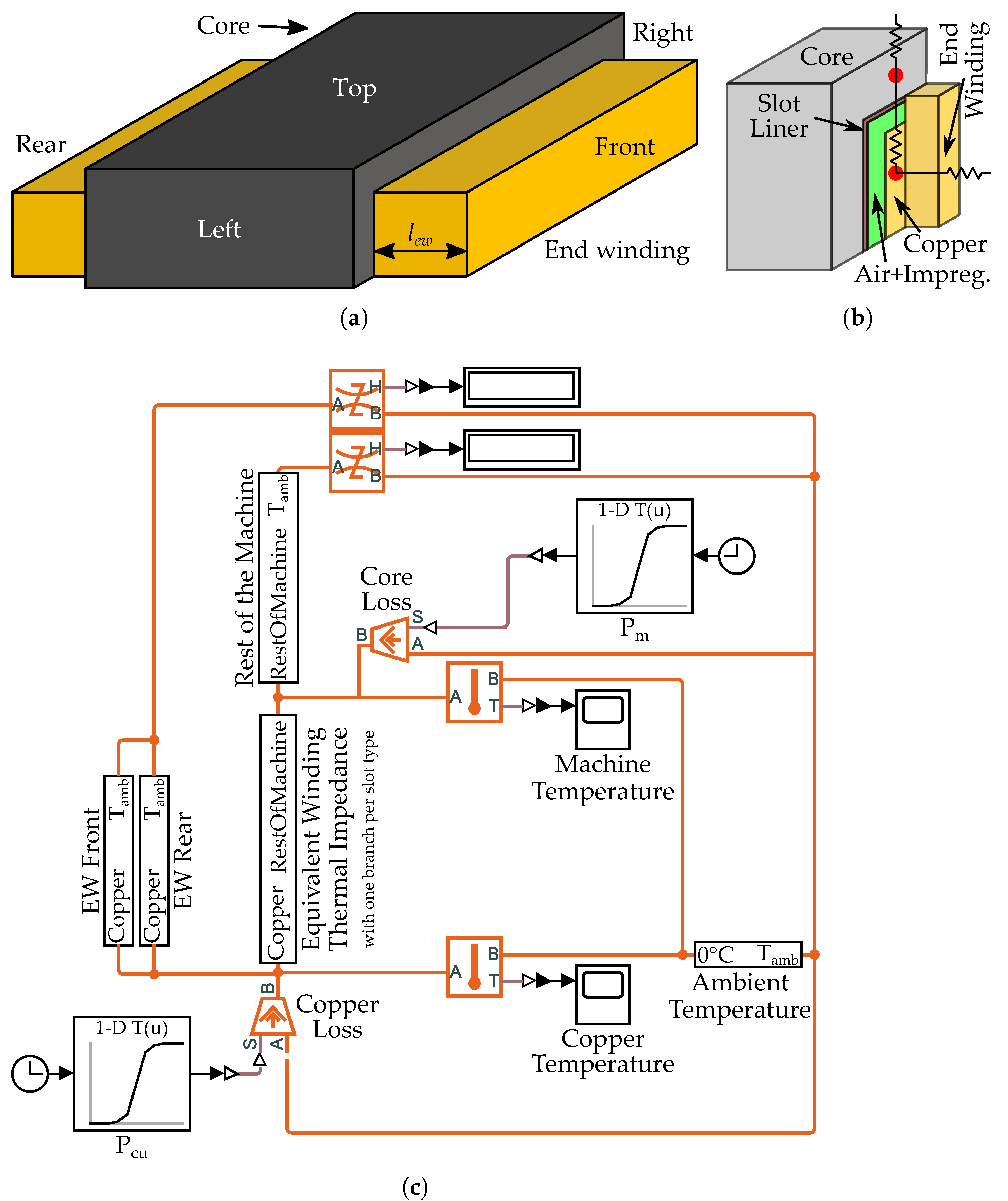
Simulink contains a toolbox that is prepared for LP thermal network modeling. Thus, it is a very appropriate software package for a fast implementation of this kind of model. Figure 1 shows the general view of the implemented network.

The toolbox has predefined elements for the three main heat transfer mechanisms: conduction, convection and radiation, and also thermal capacitances. The conductive thermal resistance $R_{cond}$ is calculated with

$$\begin{array}{cc}\hfill & R_{cond}=\frac{l}{k·A},\hfill \end{array}$$

(1)

where l, k, and A are, respectively, the thickness of the material in the direction of the heat-flow, the thermal conductivity of the material and the area of the plane of the material that is perpendicular to the heat-flow. In Simulink, the thermal resistance is calculated by the thermal resistor block itself, and the user must specify the values of the thickness, the area and the thermal conductivity.

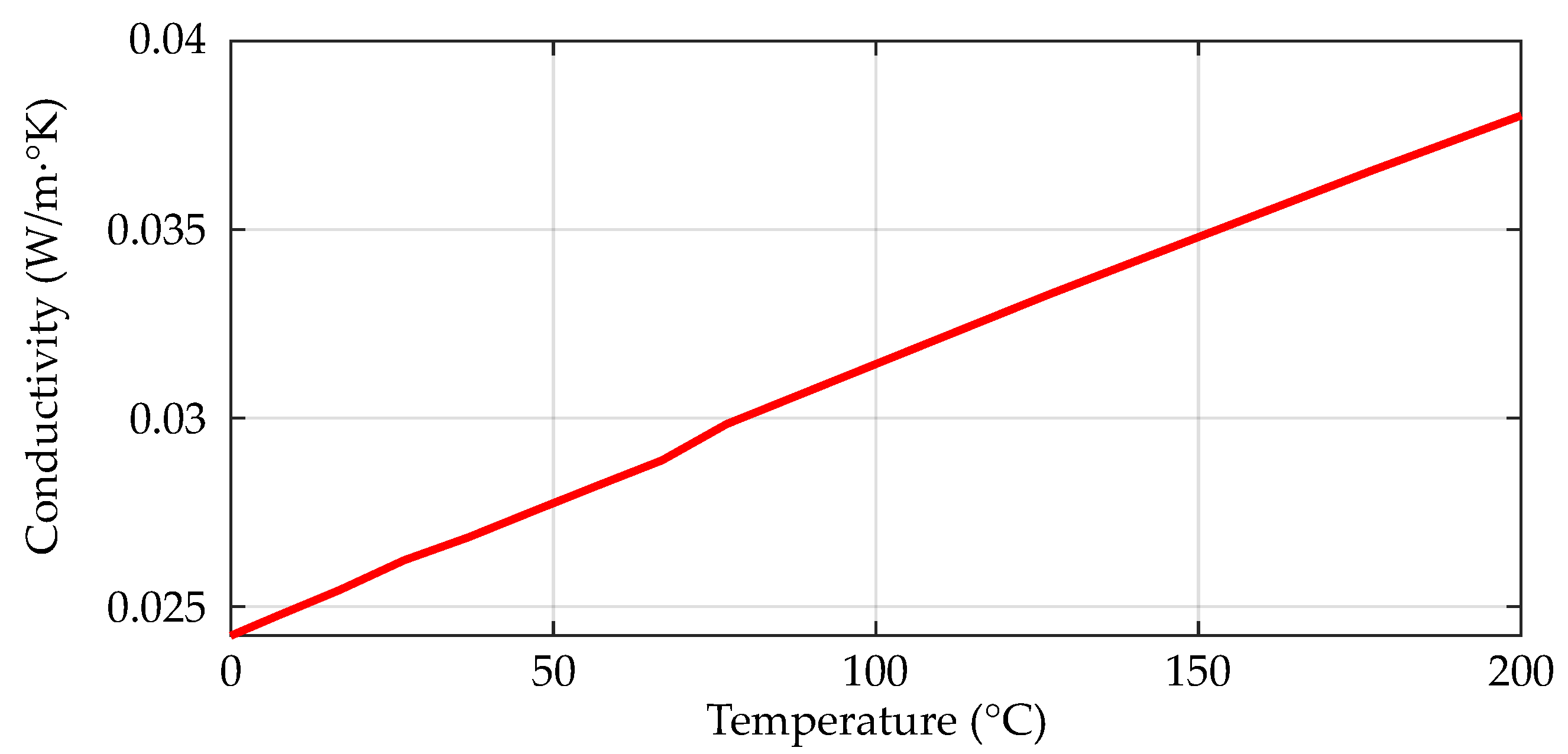
However, the block does not allow to change the thermal conductivity of an element in function of the temperature of the material. Thus, certain elements have been modeled with variable thermal resistors instead of bare conductive thermal resistances. As an example of the variation of the thermal conductivity of materials, Figure 2 displays the evolution of the thermal conductivity of air in function of its temperature.

All the thermal resistances that model some kind of air volume have been consequently modeled with the aforementioned variable resistors.

The same issue has been detected with the convective heat transfer blocks of the library. They only allow a single value for the heat transfer coefficient. Thus, variable resistors have also been used for modeling all the convective heat-flow paths. The convective resistance $R_{conv}$ is calculated with

$$\begin{array}{cc}\hfill & R_{conv}=\frac{1}{h·A},\hfill \end{array}$$

(2)

where h is the convective heat transfer coefficient, and A is the total surface area of the body in contact with the surrounding fluid. The value of h is dependant of the shape, size, and temperature of the analyzed object and also the thermal properties of the surrounding fluid, air in this case. Thus, it is not possible to use a single value to model the thermal behavior of the machine precisely enough.

Regarding radiative heat transfer, the variation of the heat-flow is only driven by the temperature difference of the elements in the heat-exchange. Thus, the pre-defined block from the library of Simulink is valid. The block establishes a heat flow Q based on

$$\begin{array}{cc}\hfill & Q=k_{rad}·A·\left(T_s^4-T_{\infty }^4\right).\hfill \end{array}$$

(3)

Here, A, $T_s$, and $T_{\infty }$ are the emitting area, the temperature of the emitting body and the temperature of the surrounding surfaces. $k_{rad}$ is the radiation coefficient. This last parameter is also changed by the shape of the objects. However, the formula for parallel plates,

$$\begin{array}{cc}\hfill & k_{rad}=\frac{\sigma }{{\displaystyle \frac{1}{{\epsilon }_1}}+{\displaystyle \frac{1}{{\epsilon }_2}}-1},\hfill \end{array}$$

(4)

has been used for all the radiating elements to simplify the calculation process.

In this way, the only configuration parameters are the area of the body and the emissivities of the emitting ${\epsilon }_1$ and receiving materials ${\epsilon }_2$. $\sigma$ is the Stefan-Boltzmann constant, 5.6704 × 10⁻⁸$\raisebox{1ex}{$\mathrm{W}$}\!\left/ \!\raisebox{-1ex}{${\mathrm{m}}^2{\mathrm{K}}^4$}\right.$.

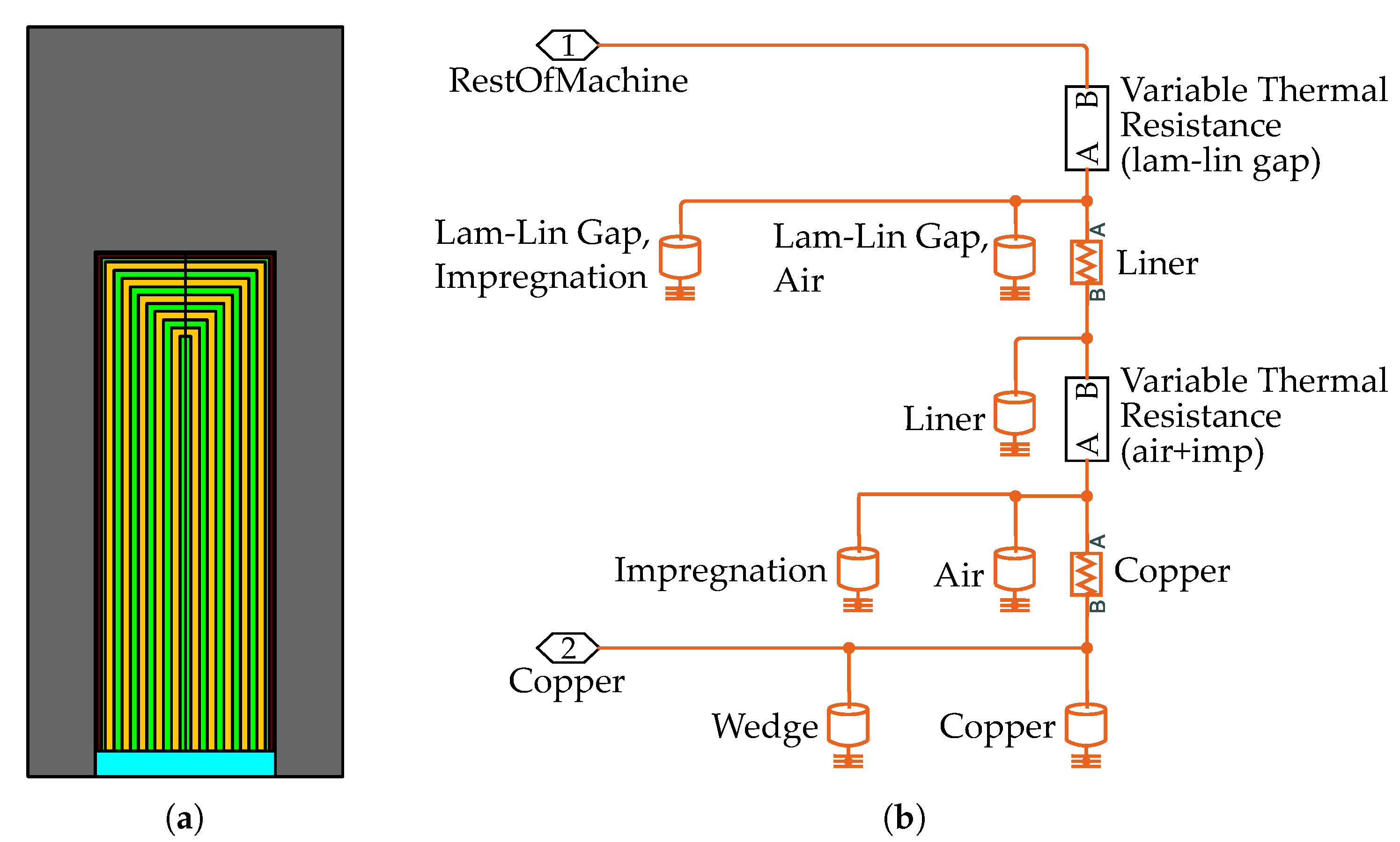
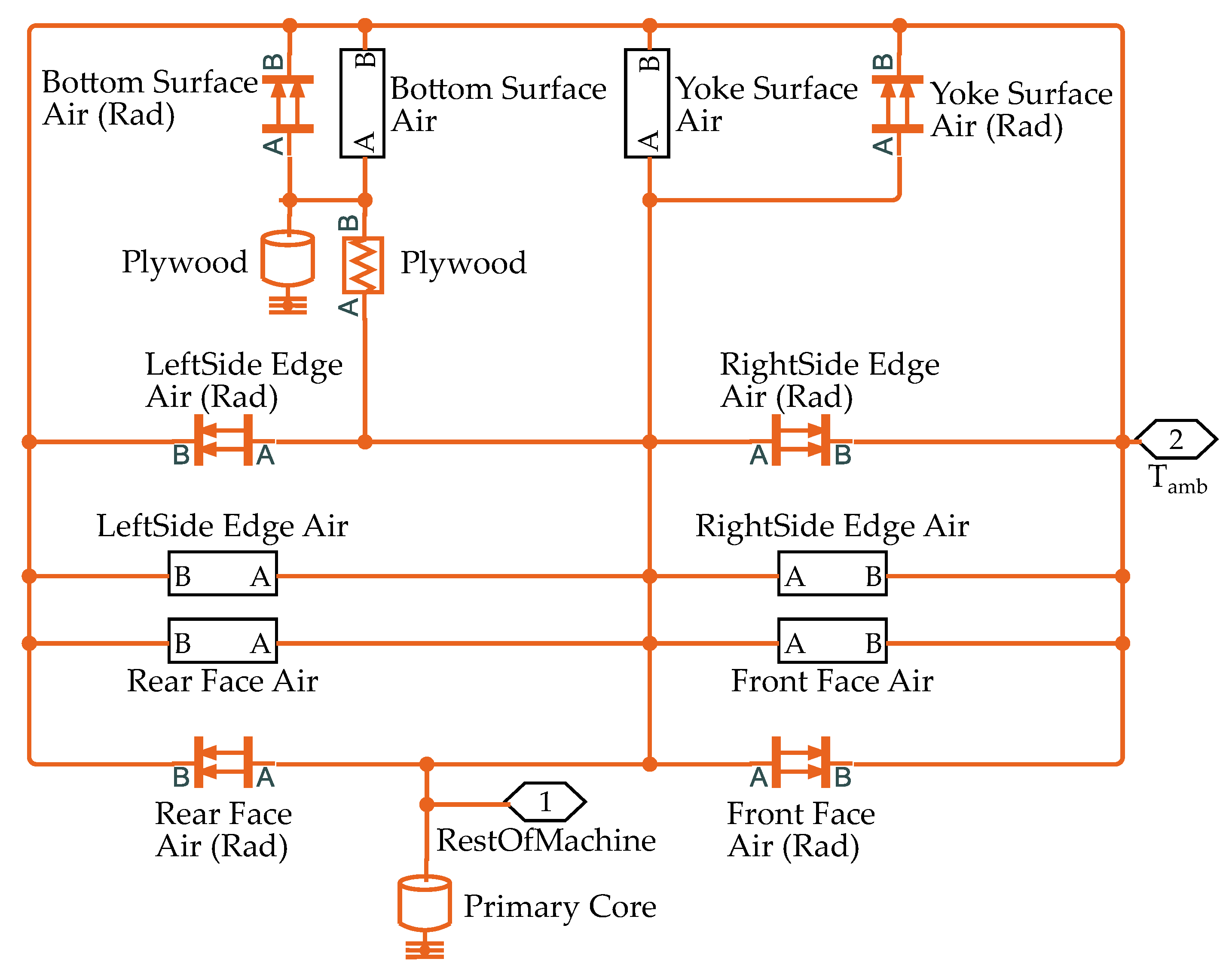
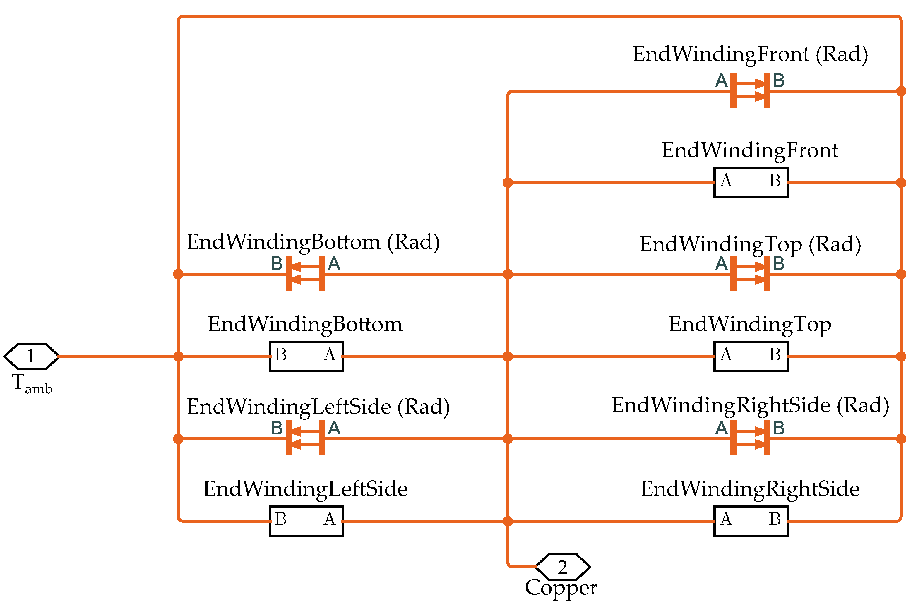
To ensure universality between different devices, the model only consists of three parts: end windings, primary core, and slot. The secondary is not contemplated by the model because, as demonstrated in Reference [22], the temperature of the secondary side of the machine is not affected by the losses if the stroke length is large enough.

3. Description of the Thermal Networks

3.1. Thermal Network of the Slot

The equivalent thermal network of the slot from Figure 3 is based on the layered winding thermal model of Motor-CAD [27]. The advantage of this model is that it is precise enough to detect hot spot problems in the windings, but the calibration of the resistance is only dependant on the thermal conductivity and the quality of the impregnation, and the fill factor of the slot.

The thickness of the copper+air+impregnation layers is the same as the diameter of the conductors of the slots. In the initialization process, the the thermal analysis tool starts from setting a low thickness for the air+impregnation layers, and this value is iteratively increased until the desired fill factor is obtained.

Each element of the slot has its own thermal resistor and capacitor as it can be seen in Figure 3b. In order to limit the height of Figure 3b, the thermal network of a machine which has a single copper and air+impregnation layer is shown in the figure.

Thanks to the winding model, it is also easy to define the values of the conductive thermal resistances. The thickness of the layers is taken as l, and A is calculated by

$$\begin{array}{cc}\hfill & A=l_{stk}·\left(2·h_{layer}+w_{layer}\right),\hfill \end{array}$$

(5)

where $h_{layer}$ and $w_{layer}$ are the average height and average width of the layers.

In the case of the air+impregnation layers, the conductive thermal resistance depends on the quality of the impregnation $q_{imp}$. This parameter contemplates the small air gaps that can appear in the impregnation due to imperfections in the manufacturing process of the machine. The value of the conductive resistance of this layer $R_{AirImp}$ is calculated following

$$\begin{array}{cc}\hfill & R_{AirImp}=q_{imp}·\frac{l}{k_{imp}·A}+\left(1-q_{imp}\right)·\frac{l}{k_{air}·A},\hfill \end{array}$$

(6)

where $k_{imp}$ and $k_{air}$ are the thermal conductivities of the impregnation and the air.

The thermal capacitances C are calculated from the mass and the specific heat capacity $c_p$ of the materials,

$$\begin{array}{cc}\hfill & C=\rho ·V·c_p.\hfill \end{array}$$

(7)

Here, $\rho$ is the density of the material of the layer, and V the total volume of the layer. The specific heat capacities, thermal conductivities, and densities of some typical materials are given in

Table 1. Thermal conductivity and specific heat capacity of typical materials.

Material	Thermal Conductivity	Specific Heat Capacity	Density	Source
Steel	30	460	7650	[28]
Wedge	0.2	1200	1000	[28]
Impregnation	0.21	1700	1400	[28]
Liner	0.21	1000	700	[28]
Copper	401	385	8933	[28]
Plywood	0.12	1200	550	[29]
Aluminium	180	963	2950	[28]

. The thermal properties of air at 1 atm are given in Appendix A.

3.2. Thermal Network of the Primary Core

As it can be seen in Table 1 and

Table A1. Thermal properties of air at 1 atm [26].

T (°K)	$\mathit{\rho }$ (kg/m3)	${\mathit{c}}_{\mathit{p}}$ (J/kg·°K)	$\mathit{\mu }$ (kg/m·s)	v (m2/s)	k (W/m·°K)	$\mathit{\alpha }$ (m2/s)	Pr
100	3.605	1039	0.00000711	$1.97\times {10}^{-6}$	0.00941	$2.51\times {10}^{-6}$	0.784
150	2.368	1012	0.00001035	$4.37\times {10}^{-6}$	0.01406	$5.87\times {10}^{-6}$	0.745
200	1.769	1007	0.00001333	$7.54\times {10}^{-6}$	0.01836	$1.03\times {10}^{-5}$	0.731
250	1.412	1006	0.00001606	$1.14\times {10}^{-5}$	0.02241	$1.58\times {10}^{-5}$	0.721
260	1.358	1006	0.00001649	$1.21\times {10}^{-5}$	0.02329	$1.71\times {10}^{-5}$	0.712
270	1.308	1006	0.00001699	$1.3\times {10}^{-5}$	0.024	$1.82\times {10}^{-5}$	0.712
280	1.261	1006	0.00001747	$1.39\times {10}^{-5}$	0.02473	$1.88\times {10}^{-5}$	0.711
290	1.217	1006	0.00001795	$1.48\times {10}^{-5}$	0.02544	$2.08\times {10}^{-5}$	0.71
300	1.177	1007	0.00001857	$1.58\times {10}^{-5}$	0.02623	$2.21\times {10}^{-5}$	0.713
310	1.139	1007	0.00001889	$1.66\times {10}^{-5}$	0.02684	$2.34\times {10}^{-5}$	0.709
320	1.103	1008	0.00001935	$1.75\times {10}^{-5}$	0.02753	$2.48\times {10}^{-5}$	0.708
330	1.07	1008	0.00001981	$1.85\times {10}^{-5}$	0.02821	$2.62\times {10}^{-5}$	0.708
340	1.038	1009	0.00002025	$1.95\times {10}^{-5}$	0.02888	$2.82\times {10}^{-5}$	0.707
350	1.008	1009	0.0000209	$2.07\times {10}^{-5}$	0.02984	$2.93\times {10}^{-5}$	0.707
400	0.8821	1014	0.0000231	$2.62\times {10}^{-5}$	0.03328	$3.72\times {10}^{-5}$	0.704
450	0.784	1021	0.00002517	$3.21\times {10}^{-5}$	0.03656	$4.57\times {10}^{-5}$	0.703
500	0.7056	1030	0.00002713	$3.85\times {10}^{-5}$	0.03971	$5.46\times {10}^{-5}$	0.704
550	0.6414	1040	0.00002902	$4.52\times {10}^{-5}$	0.04277	$6.41\times {10}^{-5}$	0.706
600	0.588	1051	0.00003082	$5.24\times {10}^{-5}$	0.04573	0.000074	0.708
650	0.5427	1063	0.00003257	$6\times {10}^{-5}$	0.04863	$8.43\times {10}^{-5}$	0.712
700	0.504	1075	0.00003425	$6.8\times {10}^{-5}$	0.05146	$9.5\times {10}^{-5}$	0.715
750	0.4704	1087	0.00003588	$7.62\times {10}^{-5}$	0.05425	0.000106	0.719
800	0.441	1099	0.00003747	$8.5\times {10}^{-5}$	0.05699	0.000118	0.723
850	0.415	1110	0.00003901	0.000094	0.05969	0.00013	0.725
900	0.392	1121	0.00004052	0.000103	0.06237	0.000142	0.728
950	0.3716	1131	0.00004199	0.000113	0.06501	0.000155	0.731
1000	0.3528	1142	0.00004343	0.000123	0.06763	0.000168	0.733
1100	0.3207	1159	0.00004622	0.000144	0.07281	0.000196	0.736
1200	0.294	1175	0.00004891	0.000166	0.07792	0.000226	0.738
1300	0.2714	1189	0.00005151	0.00019	0.08297	0.000257	0.738
1400	0.252	1201	0.00005403	0.000214	0.08798	0.000291	0.738
1500	0.2352	1211	0.00005648	0.00024	0.09296	0.000326	0.735

, the thermal conductivity of the primary core (steel) is much higher than that of the impregnation and the air. Thus, the conductive thermal resistance of the primary core has been neglected. This means that the model assumes that the temperature of the core of the machine is the same along the whole primary. Due to this simplification, the temperature of the copper is also assumed to be the same in all the slots of the same type because they are exposed to the same losses and the same thermal resistances.

The same happens with the influence of the end effect. In the reality, the amplitude of the airgap flux density is different in the edges of linear machines when compared to that in their central part. This generally creates a non-uniform distribution in the core losses. However, the influence of these non-uniform distribution of losses over the temperature is generally small. Hence, assuming a uniform temperature in the whole core of the machine, is a good approximation that helps to the simplification of the LP model.

The thermal network of the primary, which is shown in Figure 4, consists of the thermal capacity of the primary core, and convective and radiative thermal resistances to model the heat-exchange with the surrounding elements. The primary core has been separated in different elements to allow an easier calculation of the convective heat transfer coefficient and the heat exchange areas. These elements are the top and bottom surfaces, the left and right sides, and the front and rear faces. Figure 1a shows the simplified geometry that has been assumed in the construction of the model.

The first step when calculating the convective heat transfer coefficient is to determine if it is a natural convection environment or a forced convection situation. In the examples of this article, the thermal tests for the validation of the model were made statically. Hence, natural convection correlations have been applied.

Then, the thermal properties of the fluid are calculated at operating temperature,

$$\begin{array}{cc}\hfill & T_f=\frac{T_s+T_{\infty }}{2}.\hfill \end{array}$$

(8)

The temperature for the calculation of the properties of the fluid is $T_f$, and $T_s$ and $T_{\infty }$ are the temperatures of the surface and the ambient in Kelvin degrees. As both the ambient temperature and the surface temperature can change while the machine is operating, in the developed tool, the user has to specify the range of ambient and surface temperatures for the simulation. The tool then generates a matrix of $T_f$ for every possible combination. Then, the respective matrices are calculated for the properties of the fluid, based on Table A1.

Once that the properties of the surrounding fluid are obtained, the next step is to calculate the thermal volumetric expansion coefficient of the fluid $\beta$. For ideal gases, this follows

$$\begin{array}{cc}\hfill & \beta =\frac{1}{T_f}.\hfill \end{array}$$

(9)

Then, the Grashof number $G{r}_L$ and the Rayleigh $R{a}_L$ number are obtained from

$$\begin{array}{cc}\hfill & G{r}_L=\frac{g·\beta ·\left(T_s-T_{\infty }\right)·L_c^3}{v^2},\hfill \end{array}$$

(10)

and

$$\begin{array}{cc}\hfill & R{a}_L=G{r}_L·Pr,\hfill \end{array}$$

(11)

where g is the gravity in m/s², $L_c$ is the characteristic length of the surface, v is the kinematic viscosity of the fluid at the operating temperature, and $Pr$ is the Prandtl number.

Later, the Nusselt number is calculated from empirical correlations. In this case, the correlations that have been used are those presented in Reference [26] for vertical and horizontal plates. The correlations are given in

Table 2. Correlations for horizontal and vertical plates.

Configuration	Characteristic Length	$\mathit{Ra}$ Interval	Nu
Vertical Plate	Height of the plate	Whole interval	$Nu={\left\{0.825+{\displaystyle \frac{0.387·R{a}_L^{1/6}}{{\left[1+{\left(0.492/Pr\right)}^{9/16}\right]}^{8/27}}}\right\}}^2$
Hot Horizontal Plate, Top	$A/p$	104–107	$Nu=0.54·R{a}_L^{1/4}$
	p: perimeter of the plate	107–1011	$Nu=0.15·R{a}_L^{1/3}$
Hot Horizontal Plate, Bottom	$A/p$	105–1011	$Nu=0.27·R{a}_L^{1/4}$
Cold Horizontal Plate, Top	Same as bottom of hot plate
Cold Horizontal Plate, Bottom	Same as top of hot plate

.

Finally, the convective heat transfer coefficient is calculated with the obtained Nusselt number, the characteristic length of the surface, and the thermal conductivity of the fluid, obtained from the table in Appendix A, with

$$\begin{array}{cc}\hfill & h=\frac{Nu·k}{L_c}.\hfill \end{array}$$

(12)

In the final result, h is a matrix with one value for each $T_s$ and $T_{\infty }$ combination. This h is introduced to the model in lookup tables, and the model interpolates the value of the convective heat transfer coefficient depending on the ambient temperature and the temperature of each surface.

The emissivity of the materials has been extracted from Table A-18 in the appendix of Reference [26]. The given emissivity values are dependant on the finishing of the material; thus, approximated values have been selected. These values are collected in

Table 3. Emissivity of materials in the model.

Material	Emissivity
Copper	0.1
Aluminium	0.09
Steel	0.2
Surrounding surfaces (whitish)	0.3

.

3.3. Thermal Network of the End Windings

Similar to the thermal network of the primary core, the thermal conductivity of the end windings has been taken as infinite. Thus, the temperature of the copper of the end windings is the same as the average temperature of the copper in the slot. The only thermal resistances in the thermal network of the end windings (Figure 5) are those corresponding to the radiation and the convection. This is a simplification that has been made to reduce the complexity of the model. Obviously, there is an error in the calculation of the temperature of the copper in the end windings. But this can be assumed to be generally small. However, when the heat flow through the primary core is very high, the end windings can contain the actual hot-spot of the copper. Due to the simplification, this kind of hot-spot issue cannot be detected with this model.

As it can be seen in Figure 1a, the end windings have been modeled as rectangular prisms. The dimensions of the prism depend on the type of winding that is being modeled. Figure 6 shows the length of the prism (see $l_{ew}$ in Figure 1a) for a double-layer concentrated winding and a single layer distributed winding. The height of the prism is the height of the slot minus the thickness of the wedge, and the length is obtained by subtracting the width of a primary tooth to the active length of the machine. The convective heat transfer coefficients for the faces of the prisms are calculated with the process from Section 3.2.

3.4. Examples of Layouts

This tool can be used to analyze the thermal behavior of linear machines in different layouts. In this section, some examples of layouts are given, and the correlations that should be adopted in each of them are listed. An aluminium sheet has been introduced to the model in order to contemplate the mechanical system which the machines are attached to. The layouts are depicted in Figure 7.

When the layout is changed, the convective heat transfer coefficient matrix must be recalculated with the correct correlations for the defined configuration.

Table 4. Correlations for the horizontal layout.

Element	Correlation
Top of the Yoke Surface	Hot horizontal plate, top
Bottom of the Machine	Conduction to plywood
Front Side of the Yoke Surface	Vertical plate
Rear Side of the Yoke Surface	Vertical plate
Left End of the Machine	Vertical plate
Right End of the Machine	Vertical plate
Top of the End Winding Block	Hot horizontal plate, top
Bottom of the End Winding Block	Hot horizontal plate, bottom
Front side of the End Winding Block	Vertical plate
Rear side of the End Winding Block	Vertical plate
Left End of the End Winding Block	Vertical plate
Right End of the End Winding Block	Vertical plate
Plywood	Hot horizontal plate, bottom

,

Table 5. Correlations for the vertical layout.

Element	Correlation
Top of the Yoke Surface	Vertical plate
Bottom of the Machine	Vertical plate
Front Side of the Yoke Surface	Vertical plate
Rear Side of the Yoke Surface	Vertical plate
Left End of the Machine	Conduction to plywood
Right End of the Machine	Hot horizontal plate, top
Top of the End Winding Block	Vertical plate
Bottom of the End Winding Block	Vertical plate
Front side of the End Winding Block	Vertical plate
Rear side of the End Winding Block	Vertical plate
Left End of the End Winding Block	Hot horizontal plate, bottom
Right End of the End Winding Block	Hot horizontal plate, top
Plywood	Hot horizontal plate, bottom

and

Table 6. Correlations for the vertical layout with the vehicle structure.

Element	Correlation
Top of the Yoke Surface	Vertical plate
Bottom of the Machine	Vertical plate
Front Side of the Yoke Surface	Vertical plate
Rear Side of the Yoke Surface	Vertical plate
Left End of the Machine	Hot horizontal plate, bottom
Right End of the Machine	Hot horizontal plate, top
Top of the End Winding Block	Vertical plate
Bottom of the End Winding Block	Vertical plate
Front side of the End Winding Block	Vertical plate
Rear side of the End Winding Block	Vertical plate
Left End of the End Winding Block	Hot horizontal plate, bottom
Right End of the End Winding Block	Hot horizontal plate, top
Aluminium Plate	Vertical plate

show the correlations for the layouts that are displayed in Figure 7.

4. Validation of the Thermal Model

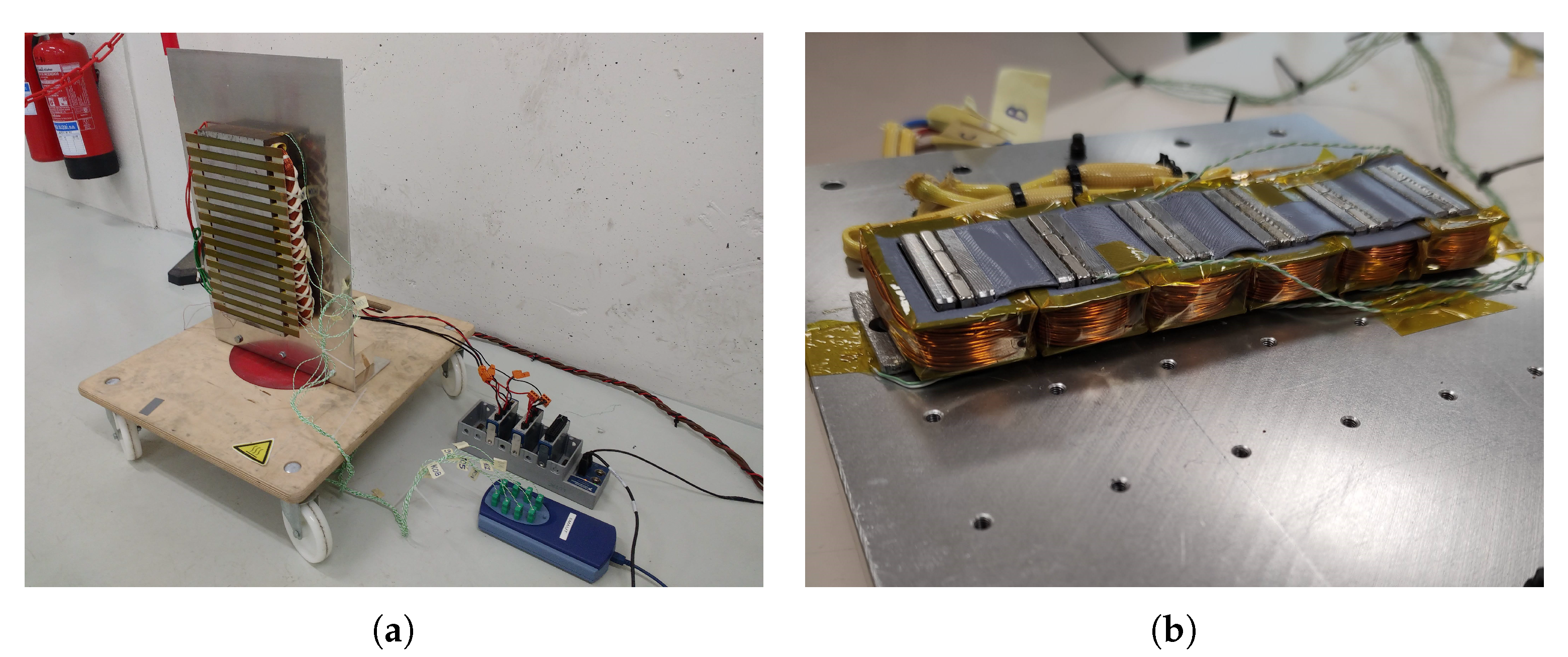
Two different linear machines have been used to validate the thermal analysis tool: a linear induction machine, and a linear switched-flux machine. The idea behind this double validation was to demonstrate the generic nature of the tool. The main parameters of the machines can be found in

Table 7. Main parameters of the prototypes for the thermal tests.

Parameter	Unit	LIM	LSFPM
Number of Slots	mm	15	7
Yoke Thickness	mm	15	2.5
Slot Height	mm	35	11.9
Primary Slot Width	mm	12	12.8
Primary Tooth Width	mm	9	4.1
Stack Length	mm	130	30
Width of the PMs	mm	-	3
Height of the PMs	mm	-	14.4
Slot Liner Thickness	mm	0.3	1
Wedge Thickness	mm	1.7	1.4
Fill Factor	-	0.35	0.3

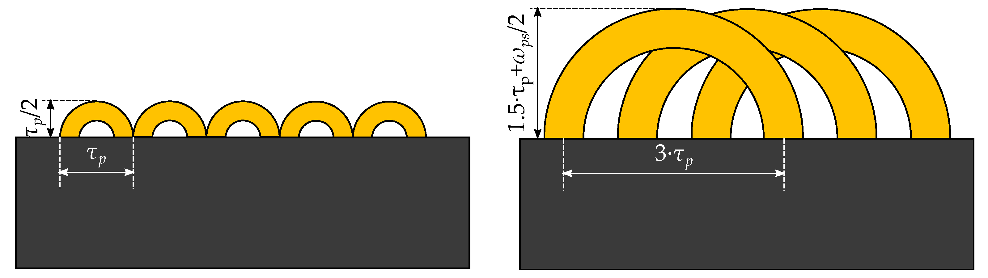
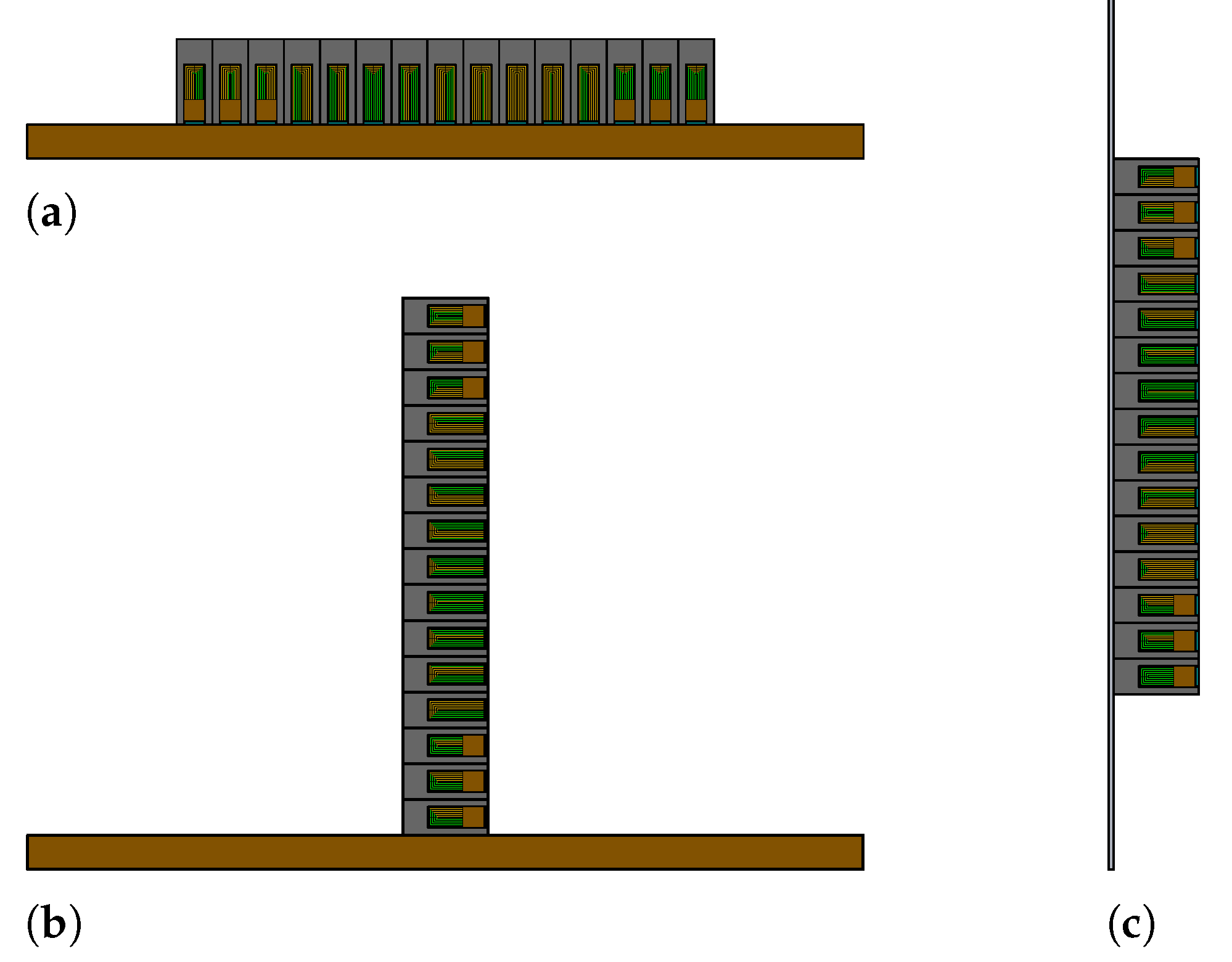
. Figure 8 shows the prototypes that were tested. The LIM has a double-layer distributed winding, and 3 slots at each side of the machine are half-filled. On the other hand, the LSFPM has a double-layer concentrated winding. The width of the edge slots is half of that of the rest of slots. The end slots are opened, so there are no teeth at the ends of the machine.

The validation of the thermal model was done via DC thermal tests. In these tests, the machine was supplied with a constant DC power, with the phase windings connected in series. This way, the magnetic losses and mechanical friction losses were avoided, and the overall heat flow of the machine was controlled directly with a power supply. The main advantage of DC thermal tests is that the only voltage in the phase coils is generated because of the resistance of the armature winding. Thus, if the current and the voltage are measured, the value of the resistance can be calculated with Ohms law,

$$\begin{array}{cc}\hfill & R=\frac{V}{I}.\hfill \end{array}$$

(13)

Then, the resistance can be used to obtain the average temperature of the copper of the machine.

The resistance of the phase windings varies according to

$$\begin{array}{cc}\hfill & R=R_0·\left[1+{\alpha }_{cu}\left(T-T_0\right)\right],\hfill \end{array}$$

(14)

where $R_0$ is the resistance of the series connected phase windings, ${\alpha }_{cu}$ is the temperature coefficient of the copper, 0.00393, and $T_0$ is the temperature at which $R_0$ was measured. Assuming that the machine is at ambient temperature at the beginning of the tests, $T_0$ can be considered to be the same as the ambient temperature. It can be deduced from (14) that the first step when testing the machines is to measure the initial resistance of the phase windings and the ambient temperature when the machine is cold.

Then, the data from the tests can be used to calculate the temperature of the copper with

$$\begin{array}{cc}\hfill & T=\frac{{\displaystyle \frac{V/I-1}{R_0}}-1}{{\alpha }_{cu}}+T_0.\hfill \end{array}$$

(15)

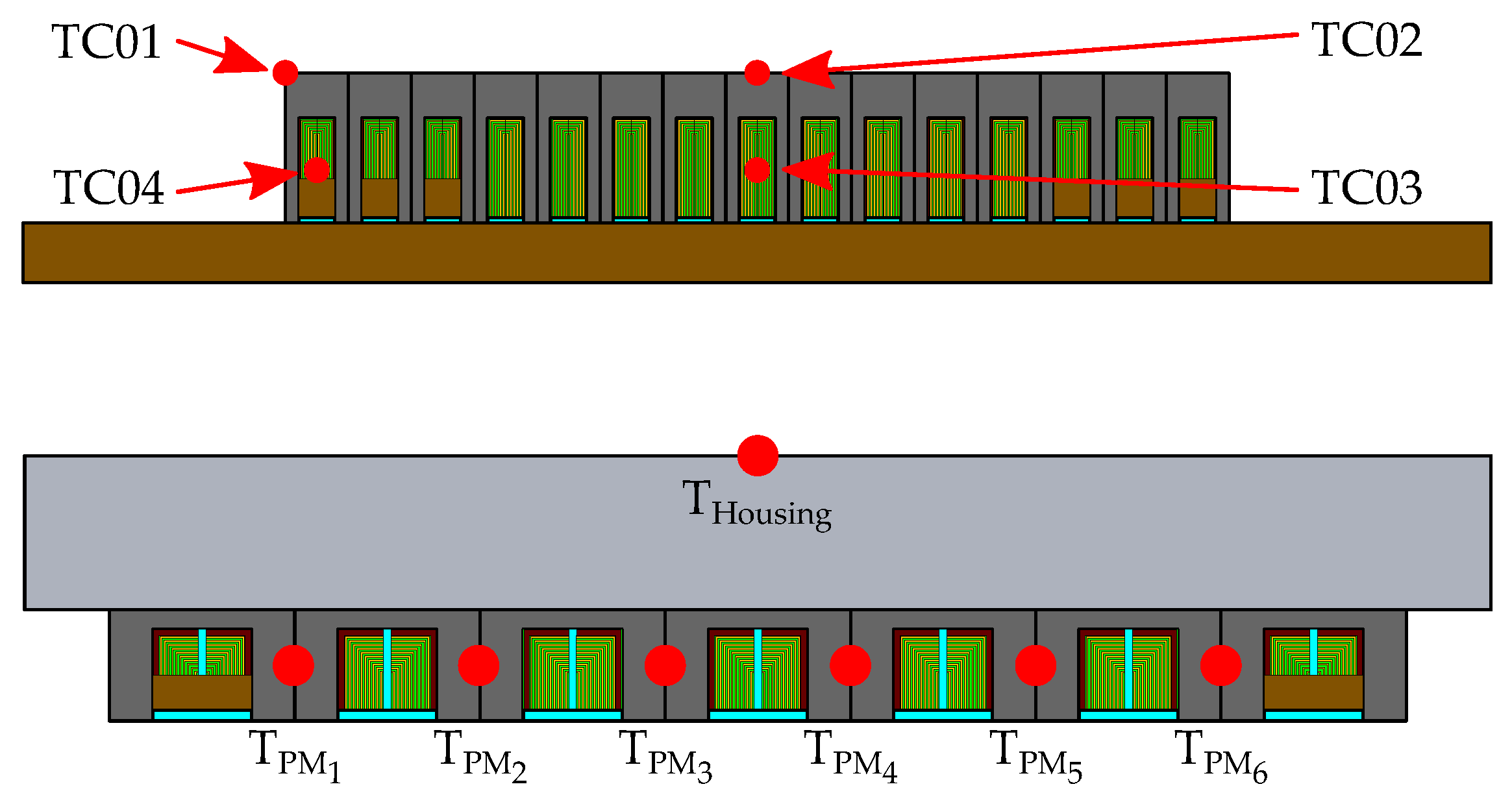
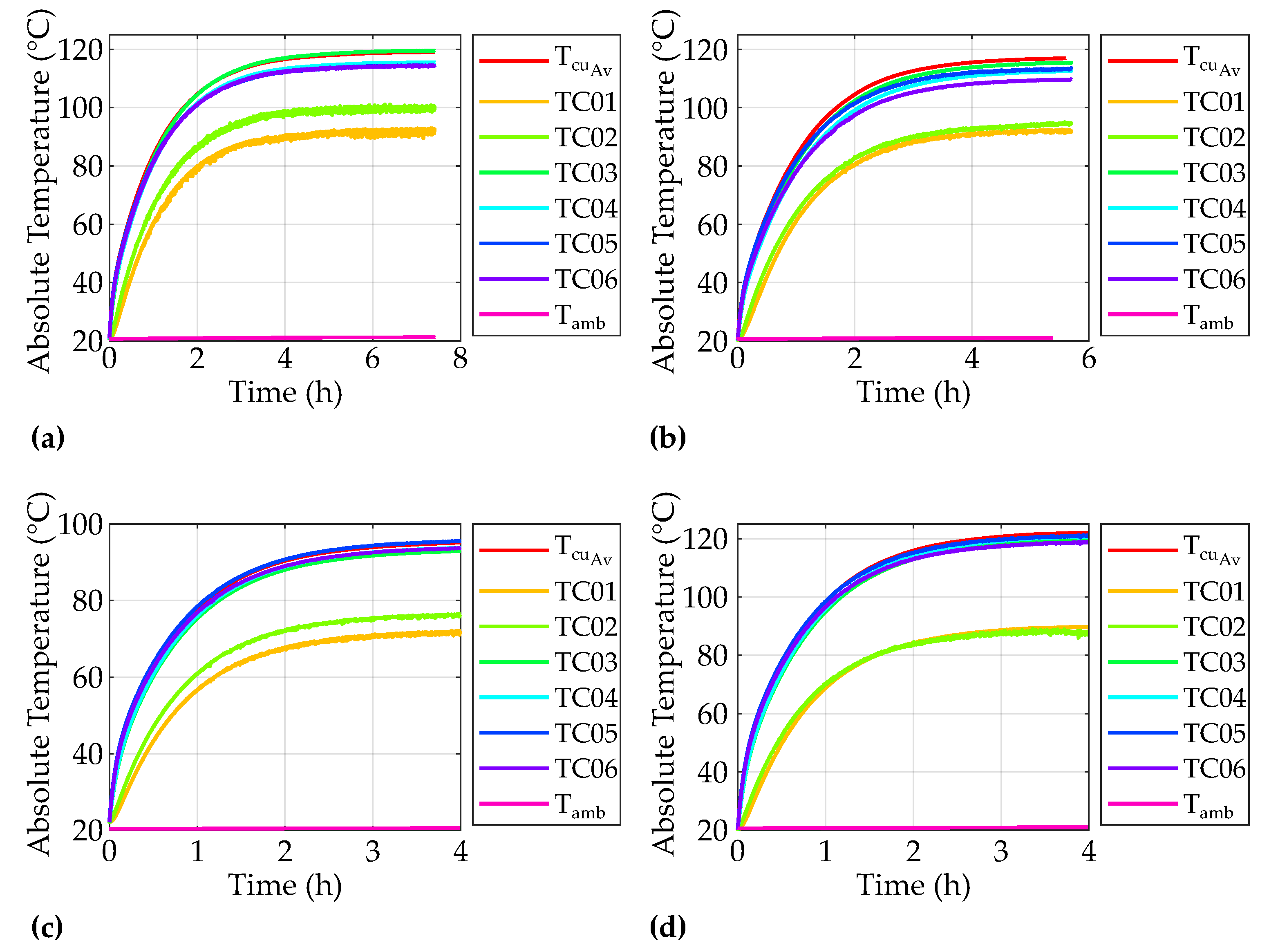
Thermocouples were used in the rest of the points where the temperature was wanted to be known. The placement of the thermocouples in the thermal tests to the LIM and the LSFPM is shown in Figure 9. And the temperatures of the machines under different conditions are given in Figure 10 and Figure 11.

In the case of the LIM, the heat dissipation capability was different depending on the layout. At 135 W, the copper of the machine reached 120 °C in the horizontal test. However, the same heat was dissipated at a lower temperature when the machine was mounted on an aluminium plate. In fact, the heat dissipation capability in the tests was 44.4% higher with the machine mounted in the aluminium frame. In this configuration, 195 W were dissipated with the copper at 120 °C. This is consistent with what was said by Staton et al. in Reference [15,16].

The aluminium sheet also helped to reduce the temperature of the core of the machine. According to

$$\begin{array}{c}\hfill \Delta T=Q·R_{th},\end{array}$$

(16)

assuming that the total slot-to-core thermal resistance $R_{th}$ remains equal, the temperature difference $\Delta T$ between the coper and the core is higher when there is a higher heat flow Q through the slot.

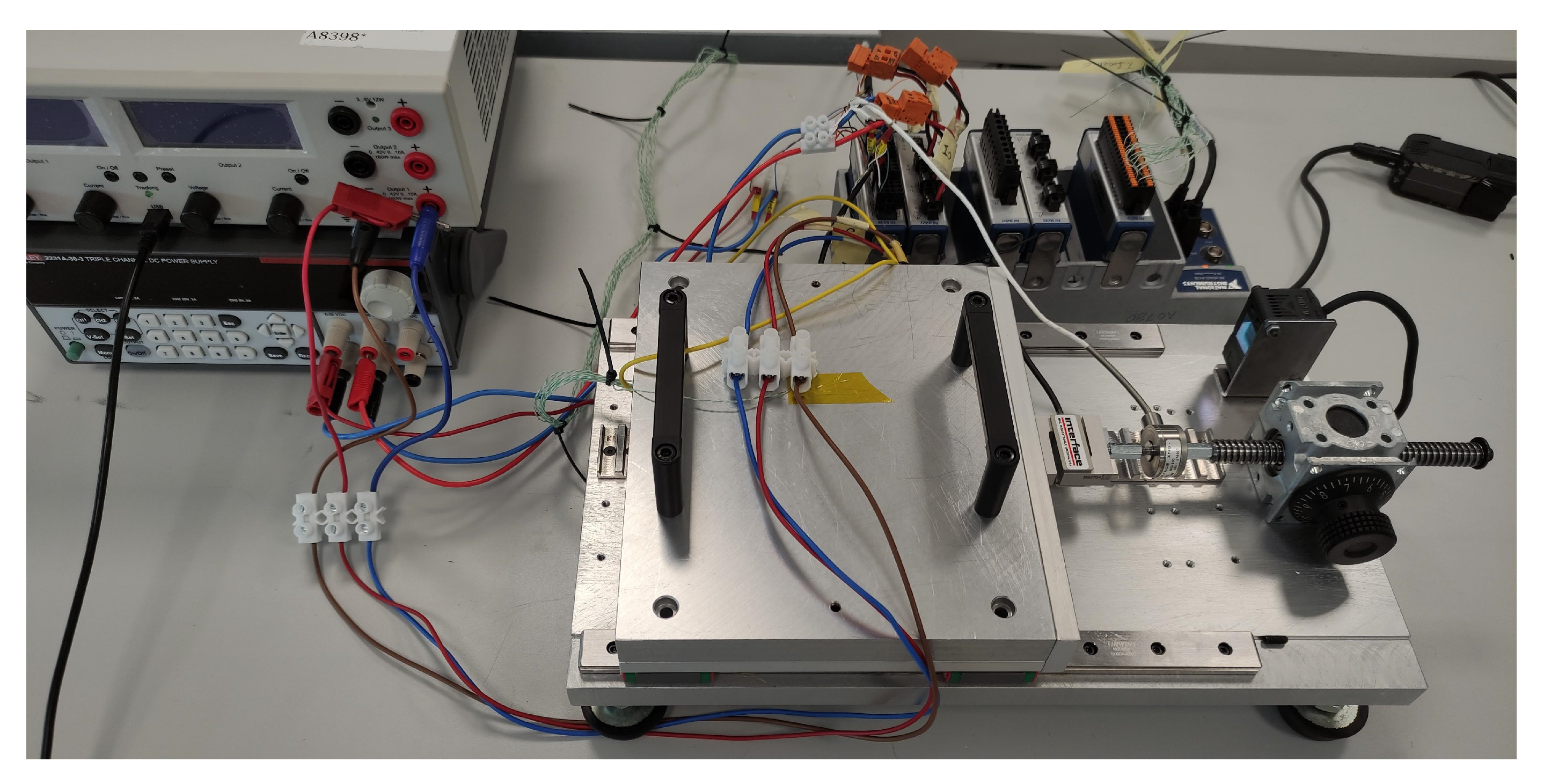
The test platform of the LSFPM can be observed in Figure 12. The coil holders of this machine were 3D printed with RS PRO’s PLA filament. This material has a vicat softening temperature of 60 °C [30]. Therefore, the maximal temperature of the copper was kept under 85 °C to ensure the integrity of the machine, and avoid an excessive deformation of the holders.

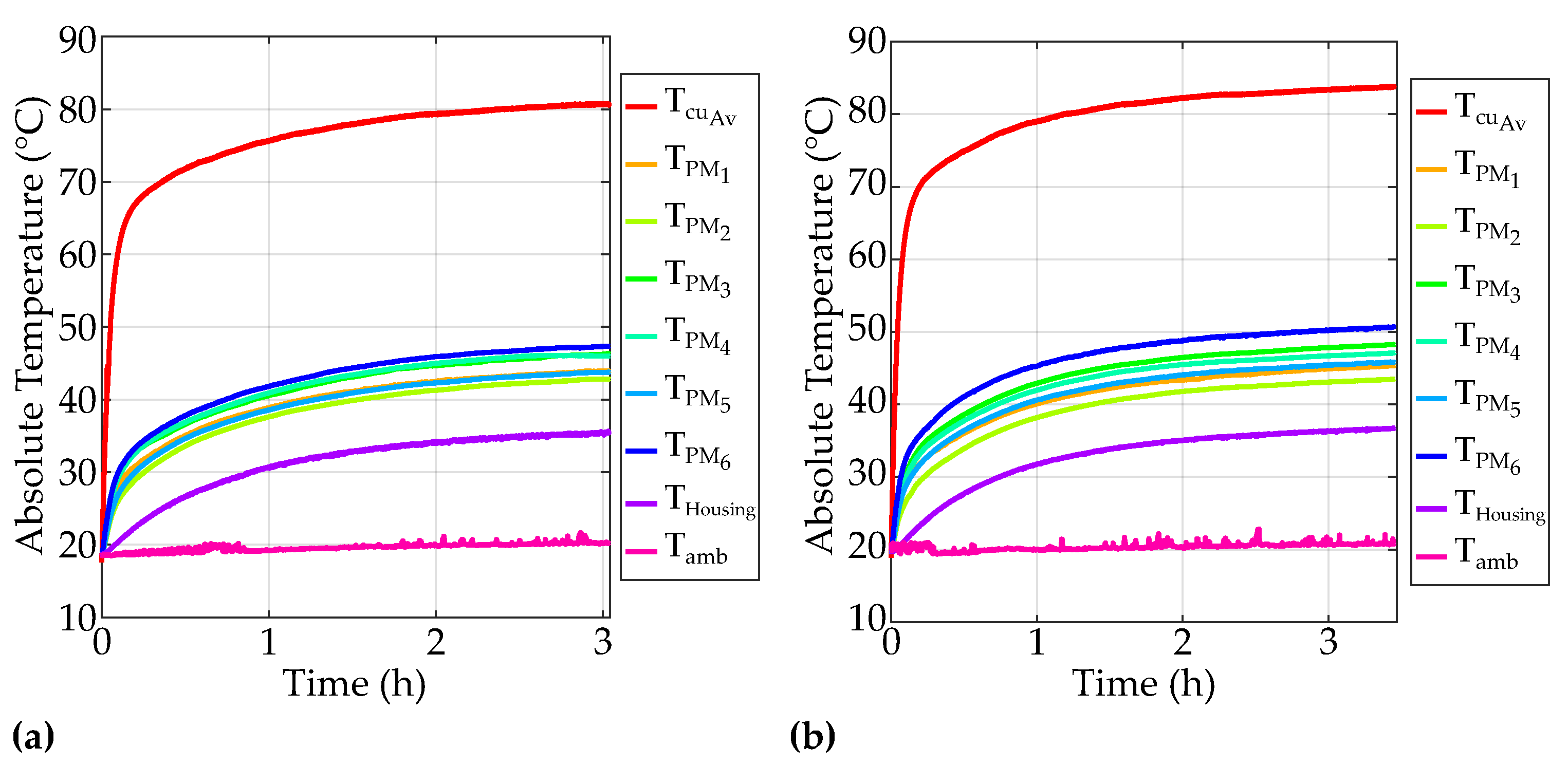
Two main temperature groups can be observed in Figure 10 and Figure 11. In order to compare the test results to the model, the temperatures of those groups, copper and core/magnets, have been averaged.

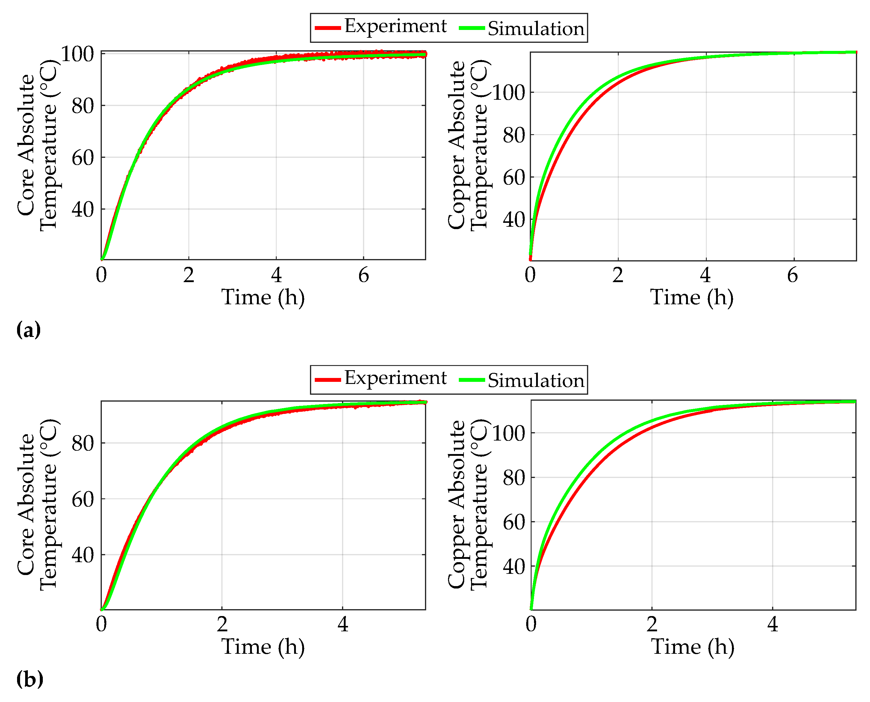
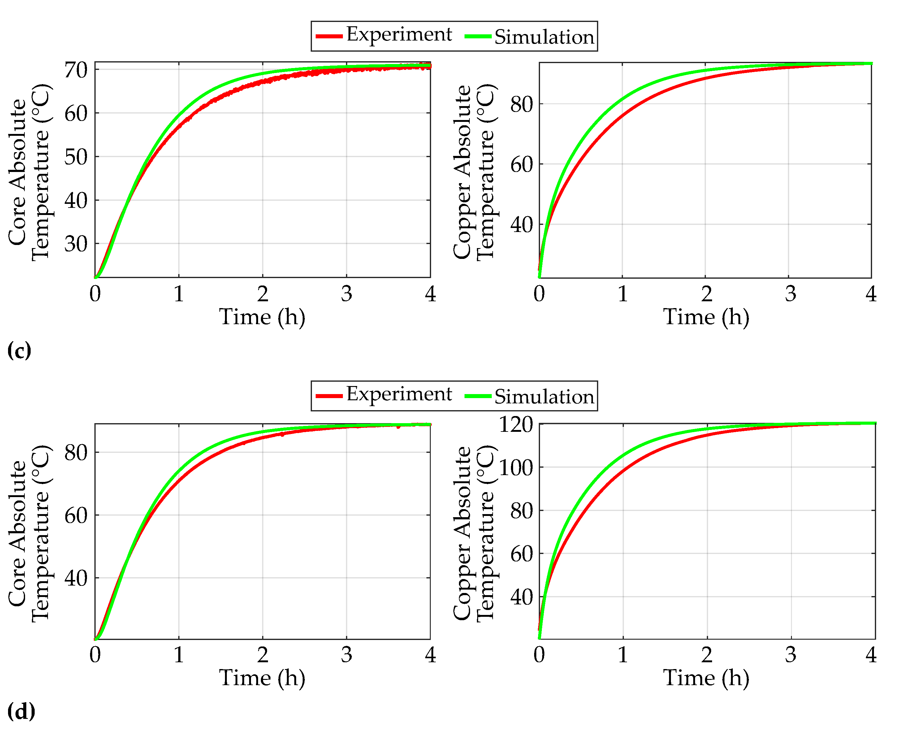
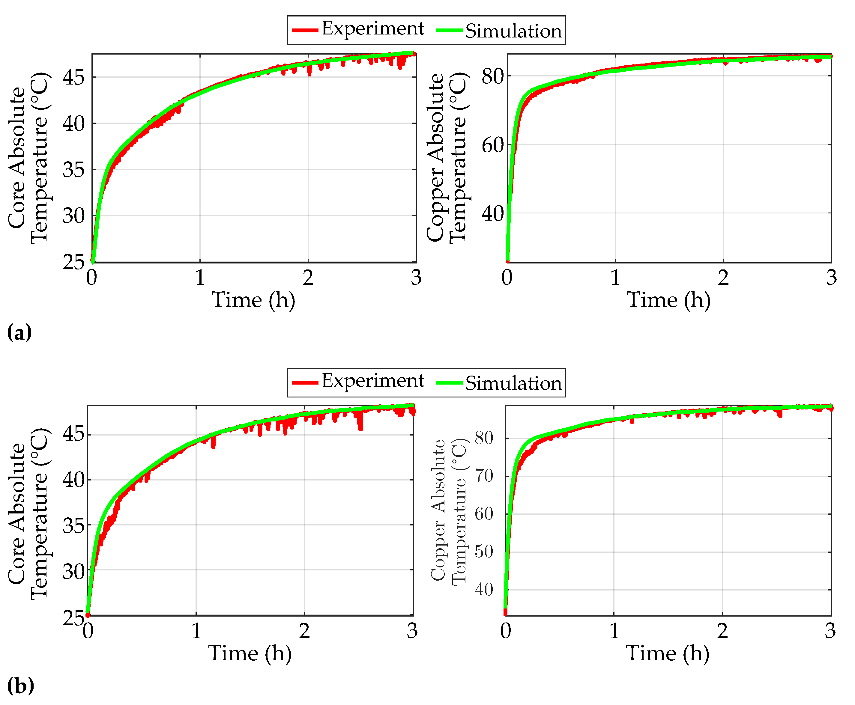
The model of each machine was calibrated by adjusting the impregnation quality and the convective heat transfer coefficients. The results of the calibrated models are compared to the results of the tests in Figure 13 and Figure 14.

5. Discussion

It is clear from Figure 13 and Figure 14 that the thermal model that is described in this article is able to predict the thermal performance of different types of linear machines precisely. The model can also predict the thermal performance of the machines in different layouts.

Although the model calculates the values of the thermal resistors based on the geometric parameters of the machine, some parameters must be calibrated.

The main calibration parameters are the quality of the impregnation, and the convective resistances of the core and the end winding. The value of the impregnation quality has to be coherent with the fabrication process of the machine. Boglietti et al. analyze the parameter sensitivity of the thermal response of some totally-enclosed fan-cooled induction machines in Reference [4]. For the impregnation goodness factor, the authors report values between 0.4 and 0.5 in machines where the impregnation process is not optimized. Thus, this value is a good starting point when there is no previous reference about the impregnation quality of the employed process. If more advanced techniques, such as vacuum impregnation, are adopted, the impregnation quality can be enhanced up to a value of 1 [15].

When calibrating the model, the impregnation quality is used to define the difference between the average temperatures of the copper and the primary core. However, a higher goodness factor will also increase the temperature of the primary core. Thus, if the temperature of the primary core gets too high, the convective heat transfer of the end windings has to be increased to reduce the heat flow through the core.

The modification of the convective heat transfer coefficients of the core is another calibration alternative. If the temperature of the core is too high, there are two ways to lower its value. The first one is to enhance the convective heat transfer coefficient of the primary core. This will increase the thermal jump from the copper to the core. If the thermal jump gets too high, then the end winding convection must be corrected.

If the resultant correction factors for the convective heat transfer are too high or too low, the impregnation quality should be reviewed. As a reference, Boglietti et al. [4] apply correction factors in a range of 0.87 to 1.35 to the convective heat transfer of the models of five different induction motors.

There is no such thing as a generic mechanical system. The mechanisms are specific to each machine and its application. Therefore, the model cannot predict the influence of the external structure of the machine. In this case, the increased heat-flow due to the aluminium plate of the LIM and the mechanical system of the LSFPM are modeled as a reduced convective thermal resistance in the surface of the yoke.

6. Conclusions

In this article, a generic thermal analysis tool was developed for linear machines in MATLAB Simulink. The model is based on simple shapes and a layered winding model to allow an easy calculation of the thermal resistance and capacitance values.

The article delivered the necessary guidelines for an easy implementation of the model in Simulink. Moreover, the calibration procedure and typical values of the calibration parameters were given. Thus, this article should serve as a reference manual for linear machine designers when implementing this kind of tool.

The model was experimentally validated with a linear induction machine and a linear switched flux machine, and the calibration procedure of the model was also explained. The results show that the model is precise for both machines, and in a handful of different scenarios. Therefore, the generic model of this tool was validated.

Simulink has been demonstrated to be a very useful tool when developing this kind of tool. The predefined blocks and the automatic solving make it very easy to implement this model. However, the convective heat transfer and the conductive thermal resistance blocks do not allow adaptive parameters. Therefore, these elements must be modeled as variable thermal resistances.

The influence of the mechanical system is not contemplated by the model. Thus, when designing a new machine, the authors would recommend to build a dummy prototype with an approximated size, and characterize the mechanical system. In this way, an accurate prediction of the thermal performance is ensured from the design stage.

References

1. Boglietti, A.; Cavagnino, A.; Staton, D.; Shanel, M.; Mueller, M.; Mejuto, C. Evolution and Modern Approaches for Thermal Analysis of Electrical Machines. IEEE Trans. Ind. Electron. 2009, 56, 871–882. [Google Scholar] [CrossRef] [Green Version]
2. Roy, P.; Towhidi, M.; Ahmed, F.; Bourgault, A.J.; Mukandan, S.; Balamurali, A.; Kar, N.C. A Comprehensive Review of Thermal Design and Analysis of Traction Motors. In Proceedings of the 2019 IEEE 28th International Symposium on Industrial Electronics (ISIE), Vancouver, BC, Canada, 12–14 June 2019; pp. 203–208. [Google Scholar] [CrossRef]
3. Boglietti, A.; Cavagnino, A.; Staton, D. Determination of critical parameters in electrical machine thermal models. IEEE Trans. Ind. Appl. 2008, 44, 1150–1159. [Google Scholar] [CrossRef]
4. Boglietti, A.; Cavagnino, A.; Staton, D.A. TEFC Induction Motors Thermal Models: A Parameter Sensitivity Analysis. IEEE Trans. Ind. Appl. 2005, 41, 756–763. [Google Scholar] [CrossRef] [Green Version]
5. San Andres, U. Thermal Optimisation of Permanent Magnet Synchronous Machines. Ph.D. Thesis, Mondragon Unibertsitatea, Arrasate, Spain, 2015. [Google Scholar]
6. Attaianese, C.; Carbone, S.; Marignetti, F. Thermal design of linear generators for wave energy converters. In Proceedings of the 19th International Conference on Electrical Machines (ICEM 2010), Rome, Italy, 6–8 September 2010; pp. 1–8. [Google Scholar] [CrossRef]
7. Chong, Y.C.; Echenique Subiabre, E.J.P.; Mueller, M.A.; Chick, J.; Staton, D.A.; McDonald, A.S. The ventilation effect on stator convective heat transfer of an axial-flux permanent-magnet machine. IEEE Trans. Ind. Electron. 2014, 61, 4392–4403. [Google Scholar] [CrossRef]
8. Rasekh, A.; Sergeant, P.; Vierendeels, J. Convective heat transfer prediction in disk-type electrical machines. Appl. Therm. Eng. 2015, 91, 778–790. [Google Scholar] [CrossRef]
9. Nategh, S.; Zhang, H.; Wallmark, O.; Boglietti, A.; Nassen, T.; Bazant, M. Transient Thermal Modeling and Analysis of Railway Traction Motors. IEEE Trans. Ind. Electron. 2019, 66, 79–89. [Google Scholar] [CrossRef]
10. Rocca, S.L.; Pickering, S.J.; Eastwick, C.N.; Gerada, C.; Ronnberg, K. Numerical Study on the Impact of End Windings Porosity on the Fluid Flow and Heat Transfer in a Totally Enclosed Fan-Cooled Electrical Machine. In Proceedings of the 2019 IEEE International Electric Machines & Drives Conference (IEMDC), San Diego, CA, USA, 12–15 May 2019; pp. 2138–2143. [Google Scholar] [CrossRef]
11. Melka, B.; Smolka, J.; Hetmanczyk, J.; Lasek, P. Numerical and experimental analysis of heat dissipation intensification from electric motor. Energy 2019, 182, 269–279. [Google Scholar] [CrossRef]
12. Sanandres, U.; Almandoz, G.; Poza, J.; Ugalde, G. Design of cooling systems using computational fluid dynamics and analytical thermal models. IEEE Trans. Ind. Electron. 2014, 61, 4383–4391. [Google Scholar] [CrossRef]
13. Nituca, C.; Chiriac, G.; Cuciureanu, D.; Dumitrescu, C.; Zhang, G.; Han, D.; Plesca, A. Thermal modeling of a linear induction motor used to drive a power supply system for an electric locomotive. Therm. Sci. 2019, 23, 589–597. [Google Scholar] [CrossRef]
14. Nituca, C. Thermal Analisys for a Double Sided Linear Induction Motor. Eur. Sci. J. 2013, 9, 38–50. [Google Scholar]
15. Staton, D. Thermal computer aided design-advancing the revolution in compact motors. In Proceedings of the IEEE International Electric Machines and Drives Conference (Cat. No.01EX485), IEMDC 2001, Cambridge, MA, USA, 17–20 June 2001; pp. 858–863. [Google Scholar] [CrossRef]
16. Staton, D.A. Servo Motor Size Reduction—Need for Thermal CAD. In Proceedings of the Drives & Controls 2001 Conference, London, UK, 13–15 March 2001. [Google Scholar]
17. Amoros, J.G.; Andrada, P.; Blanque, B. An analytical approach to the thermal design of a double-sided linear switched reluctance motor. In Proceedings of the 19th International Conference on Electrical Machines (ICEM 2010), Rome, Italy, 6–8 September 2010; pp. 4–7. [Google Scholar] [CrossRef]
18. Song, S.; Zhang, M.; Ge, L.; Wang, L. Multiobjective optimal design of switched reluctance linear launcher. IEEE Trans. Plasma Sci. 2015, 43, 1339–1345. [Google Scholar] [CrossRef]
19. Zhang, S.; Zheng, P.; Yu, B.; Cheng, L.; Wang, M. Thermal analysis and experimental verification of a staggered-teeth transverseflux permanent-magnet linear machine. IET Electr. Power Appl. 2018, 12, 1048–1057. [Google Scholar] [CrossRef]
20. Bertola, L.; Cox, T.; Wheeler, P.; Garvey, S.; Morvan, H. Thermal Design of Linear Induction and Synchronous Motors for Electromagnetic Launch of Civil Aircraft. IEEE Trans. Plasma Sci. 2017, 45, 1146–1153. [Google Scholar] [CrossRef]
21. Sarapulov, F.N.; Goman, V.V. Development of mathematical models of thermal processes in linear asynchronous motors. Russ. Electr. Eng. 2009, 80, 431–435. [Google Scholar] [CrossRef]
22. Jimenez, J. Diseño De Motores Lineales Síncronos Miniaturizados Para El Accionamiento De Puertas Automáticas. Ph.D. Thesis, Universidad de Navarra, Donostia/San Sebastián, Spain, 2013. [Google Scholar]
23. Tessarolo, A.; Bruzzese, C. Computationally efficient thermal analysis of a low-speed high-thrust linear electric actuator with a three-dimensional thermal network approach. IEEE Trans. Ind. Electron. 2015, 62, 1410–1420. [Google Scholar] [CrossRef]
24. Wang, D.; Zhang, D.; Du, X.; Wang, X. Thermal Identification, Model, and Experimental Validation of a Toroidally Wound Mover Linear-Switched Reluctance Machine. IEEE Trans. Magn. 2018, 54, 1–5. [Google Scholar] [CrossRef]
25. Kylander, G. Thermal Modelling of Small Cage Induction Motors. Ph.D. Thesis, School of Electrical and Computer Engineering, Chalmers University of Technology, Göteborg, Sweden, 1995. [Google Scholar]
26. Çengel, Y.A. Transferencia de Calor y Masa—Un Enfoque Práctico; McGraw Hill: Ciudad de México, México, 2007. [Google Scholar]
27. Staton, D.; Boglietti, A.; Cavagnino, A. Solving the more difficult aspects of electric motor thermal analysis in small and medium size industrial induction motors. IEEE Trans. Energy Convers. 2005, 20, 620–628. [Google Scholar] [CrossRef] [Green Version]
28. Motor Design Ltd. Motor-CAD. Available online: https://www.motor-design.com/motor-cad (accessed on 22 March 2021).
29. Lienhard, J.H., IV; Lienhard, J.H., V. A Heat Transfer Textbook, 3rd ed.; Phlogiston Press: Cambridge, MA, USA, 2002. [Google Scholar]
30. RS PRO, PLA Filament for FDM 3D Printer, Product Datasheet. Available online: https://docs.rs-online.com/2453/0900766b8157ce89.pdf (accessed on 23 April 2021).
Figure 1. General view of the thermal model. (a) Simplified geometry. (b) Modeled elements. (c) General view of the thermal LP network.
Applsci 11 05818 g001
Figure 2. Thermal conductivity of air at 1 atm in function of the temperature, adapted from Reference [26].
Applsci 11 05818 g002
Figure 3. (a) Implemented layered winding model. Primary core (gray), copper layers (yellow), air+impregnation layers (green), slot liner (maroon), and wedge (blue). (b) Thermal network of the slot.
Applsci 11 05818 g003
Figure 4. Thermal network for the primary core.
Applsci 11 05818 g004
Figure 5. Thermal network for the end windings.
Applsci 11 05818 g005
Figure 6. Modeled size for the end windings. Double-layer concentrated winding (left) single-layer distributed winding (right).
Applsci 11 05818 g006
Figure 7. Example layouts: (a) horizontal, (b) vertical, and (c) vertical with vehicle structure.
Applsci 11 05818 g007
Figure 8. Photos of the thermal test prototypes. (a) Linear induction machine. (b) Linear switched-flux machine.
Applsci 11 05818 g008
Figure 9. Placement of the thermocouples. LIM (top); LSFPM (bottom).
Applsci 11 05818 g009
Figure 10. Results of the thermal tests of the LIM. (a) Horizontal at 135 W. (b) Vertical at 135 W. (c) Vertical with aluminium plate at 135 W. (d) Vertical with aluminium plate at 195 W.
Applsci 11 05818 g010
Figure 11. Results of the thermal tests of the LSFPM. (a) Horizontal at 20 W. (b) Vertical at 21 W.
Applsci 11 05818 g011
Figure 12. Thermal test setup of the LSFPM.
Applsci 11 05818 g012
Figure 13. LIM thermal test result vs model response. (a) Horizontal test. (b) Vertical test. (c) Vertical test with aluminium plate at 135 W. (d) Vertical test with aluminium plate at 195 W.
Applsci 11 05818 g013aApplsci 11 05818 g013b
Figure 14. LSFPM thermal test result vs model response. (a) Horizontal test. (b) Vertical test.
Applsci 11 05818 g014