A Comprehensive Application of Machine Learning Techniques for Short-Term Solar Radiation Prediction

Abstract

Forecasting the output power of solar PV systems is required for the good operation of the power grid and the optimal management of energy fluxes occurring in the solar system. Before forecasting the solar system’s output, it is essential to focus on the prediction of solar irradiance. In this paper, the solar radiation data collected for two years in a certain place in Jiangsu in China are investigated. The objective of this paper is to improve the ability of short-term solar radiation prediction. Firstly, missing data are recovered through the means of matrix completion. Then the completed data are denoised via robust principal component analysis. To reduce the influence of weather types on solar radiation, spectral clustering is adopted by fusing sparse subspace representation and k-nearest-neighbor to partition the data into three clusters. Next, for each cluster, four neural networks are established to predict the short-term solar radiation. The experimental results show that the proposed method can enhance the solar radiation accuracy.

1. Introduction

In recent years, the scale of renewable energy power generation has expanded rapidly. Many countries are considering incorporating renewable energy into the grid [1]. Solar energy has become one of the main sources of renewable energy [2]. The narrow definition of solar energy is solar radiation [3]. Broadly speaking, solar energy also includes other forms of energy converted from the solar radiation, such as coal, oil, natural gas, hydropower, wind energy, biological energy, etc. Solar radiation is affected by the seasons and geography, and has obvious discontinuities and uncertainties [4,5]. These characteristics are the reason that the focus of prediction must be on solar radiation prior to predicting the output of a solar system.

Photovoltaic (PV) power generation is typically divided into two forms: off-grid and grid-connected. With the maturity and development of grid-connected PV technology, grid-connected PV power generation has become a mainstream trend [6]. The capacity of large-sale centralized grid-connected PV power generation systems is rapidly increasing. However, the output power of grid-connected PV power generation systems is inherently intermittent and uncontrollable. These intrinsic characteristics cause an adverse impact on the grid and seriously restrict grid-connected PV power generation [7].

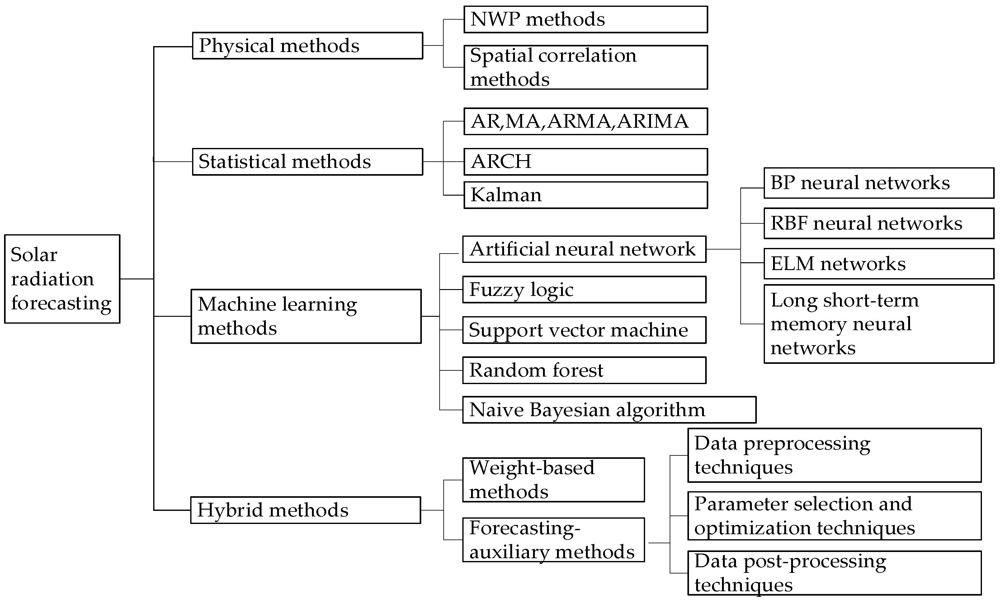
At present, research on solar radiation prediction has become more and more extensive and in depth. Among various prediction methods, the simplest is the persistence method which assumes that the future solar radiation is equal to the current solar radiation. Other solar radiation prediction methods can be classified into four categories: physical methods, statistical methods, machine learning methods and hybrid methods [8,9,10,11]. Figure 1 briefly summarizes four types of prediction methods on solar radiation.

Among the four categories in Figure 1, the physical methods establish the solar power generation forecast model according to the geographical environment and weather data (such as temperature, humidity, pressure, etc.) [8]. These methods can be further grouped into two subcategories: numerical weather prediction (NWP) methods [12] and spatial correlation methods [13]. NWP methods use numerical simulation to predict, that is, mathematical and physical models are applied on analyzing atmospheric conditions, and high-speed computers are utilized to forecast solar radiation [14]. Under normal conditions, NWP methods probably take a long time to predict [15]. Moreover, the meteorological and environmental factors in NWP methods are the most complicated and difficult to make accurate decisions [8,16]. In current research, it has always been difficult to improve forecast accuracy. The spatial correlation methods harness the spatial correlation of solar radiation to predict solar energy of several places. It should be noted that spatial correlation methods require rich historical data to simulate complex temporal and spatial changes. In summary, NWP methods and other physical models are not suitable for use in short-term cases and in small areas, owing to long runtimes. Meanwhile, they have high demands on computing resources.

The forecasting of solar radiation intensity and solar energy based on historical experimental data is more suitable for short-term prediction [17]. Statistical methods can be mainly classified into moving average (MA), autoregressive (AR) and autoregressive moving average (ARMA), autoregressive integrated moving average (ARIMA), autoregressive conditional heteroscedasticity (ARCH) and Kalman filtering [18,19]. The above models have fast calculation speeds, a strong interpretation ability and simple structures. However, statistical methods establish rigorous mathematical relationships between the inputs and outputs, which means that they cannot learn and change prediction strategies. In addition, a large amount of historical recording is required. As a result, it is almost impossible to capture nonlinear behavior in a time series, so the prediction accuracy may be decreased as time goes by.

With the booming development of artificial intelligence, the application of machine learning technology on predicting PV generation is becoming more popular. These advanced techniques include artificial neural networks (ANN), fuzzy logic (FL), support vector machines (SVM), random forest (RF) and the naive Bayesian algorithm [20,21,22,23,24,25]. The main principle of machine learning methods is as follows. Among them, artificial neural networks are a frequently used method, mainly containing black-propagation (BP) neural networks [26], radial basis function (RBF) neural networks [27], extreme learning machine (ELM)networks [28], and long short-term memory (LSTM) neural networks [29]. Several types of elements affecting solar radiation are determined firstly as the input features, then a nonlinear and highly complex mapping relationship is constructed. Finally, the model parameters are learned according to historical data. Traditional statistical methods cannot attain the above complex representation in most situations. In contrast, machine learning methods can overcome this deficiency.

Hybrid methods of solar radiation prediction mainly consist of weight-based methods and prediction-assisted methods. The former type is a combined model composed of multiple single models with the same structure. Each model gives a unique prediction, and the weighted average of the prediction results of all models is regarded as the final prediction result [30,31]. Unlike weight-based methods, prediction assistance methods usually include two models, one for power prediction and the other for auxiliary processes, such as data filtering, data decomposition, optimal parameter selection, and residual evaluation. According to the auxiliary technology, the forecast methods can be further divided into three groups: data preprocessing techniques, parameter optimization techniques, and residual calibration techniques. Among them, data preprocessing techniques are the commonly used methods, and they mainly include principal component analysis (PCA) and cluster analysis [31,32], the wavelet transform (WT) [33], empirical mode decomposition (EMD) [34] and variational mode decomposition (VMD) [35], etc. Reasonable selections of preprocessing methods can reduce the negative impact of the systematic error on prediction accuracy to a certain extent. In summary, each single model has its advantages and disadvantages, and the hybrid model combines advantages of different methods to obtain a better prediction performance.

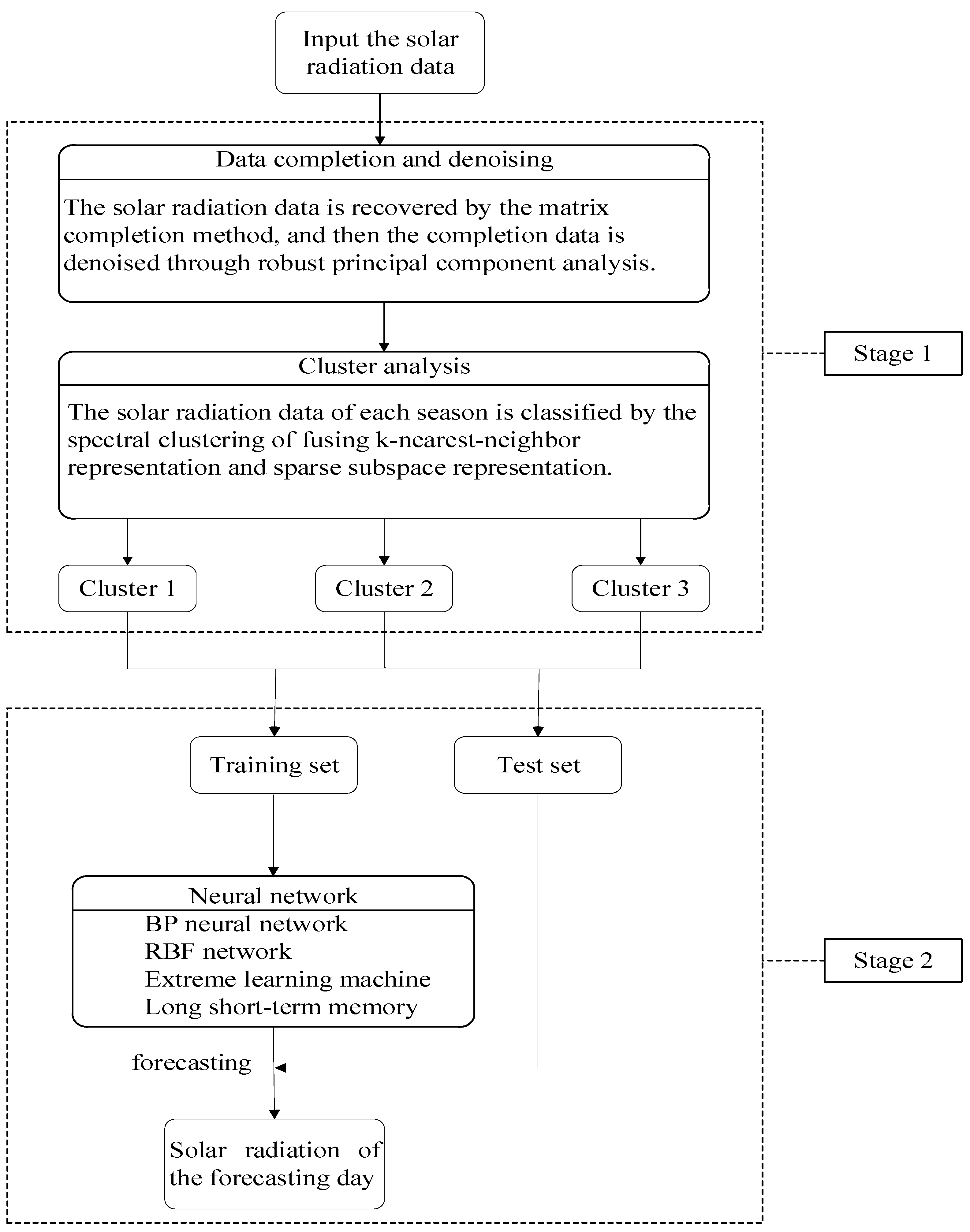
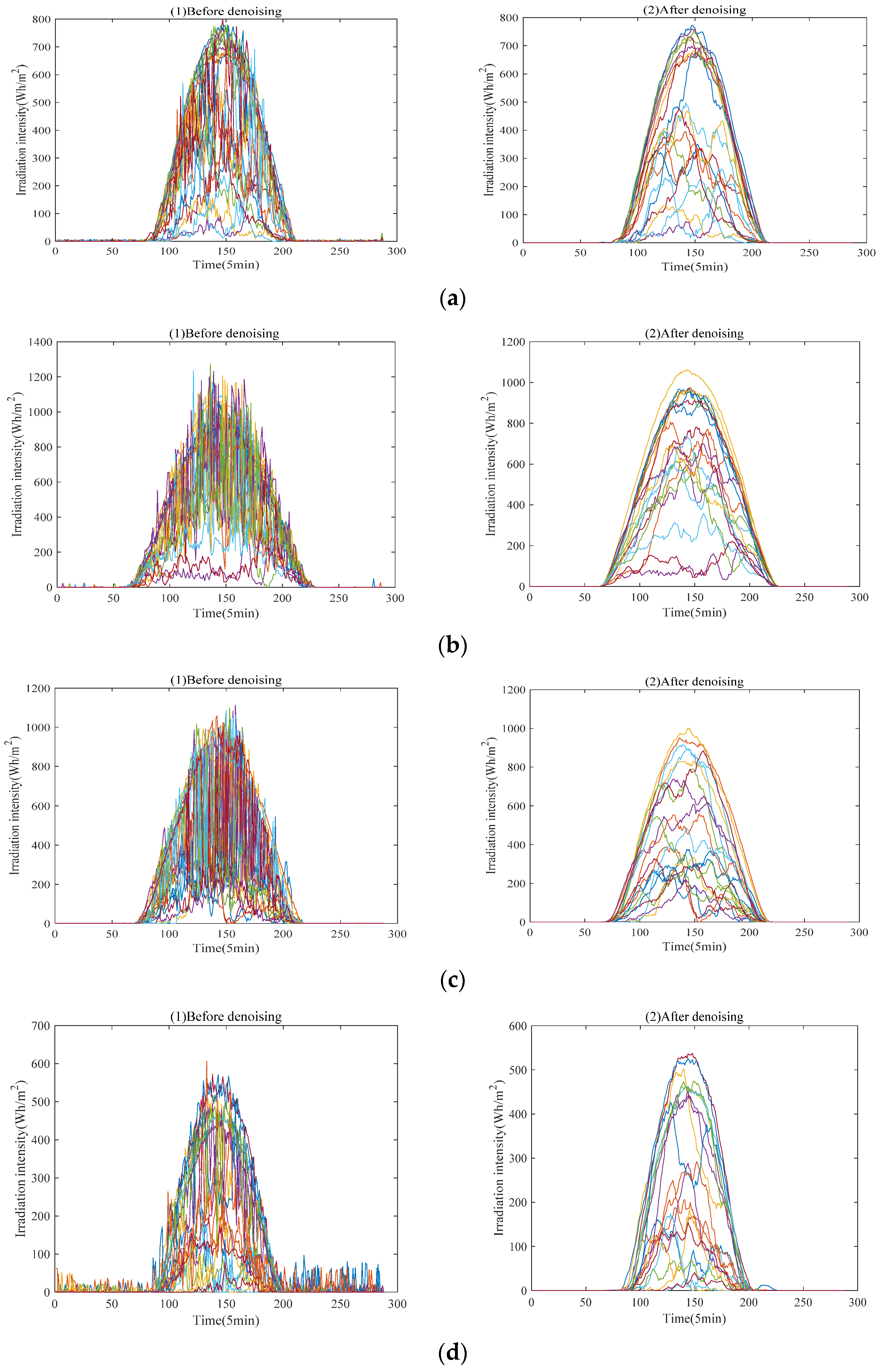
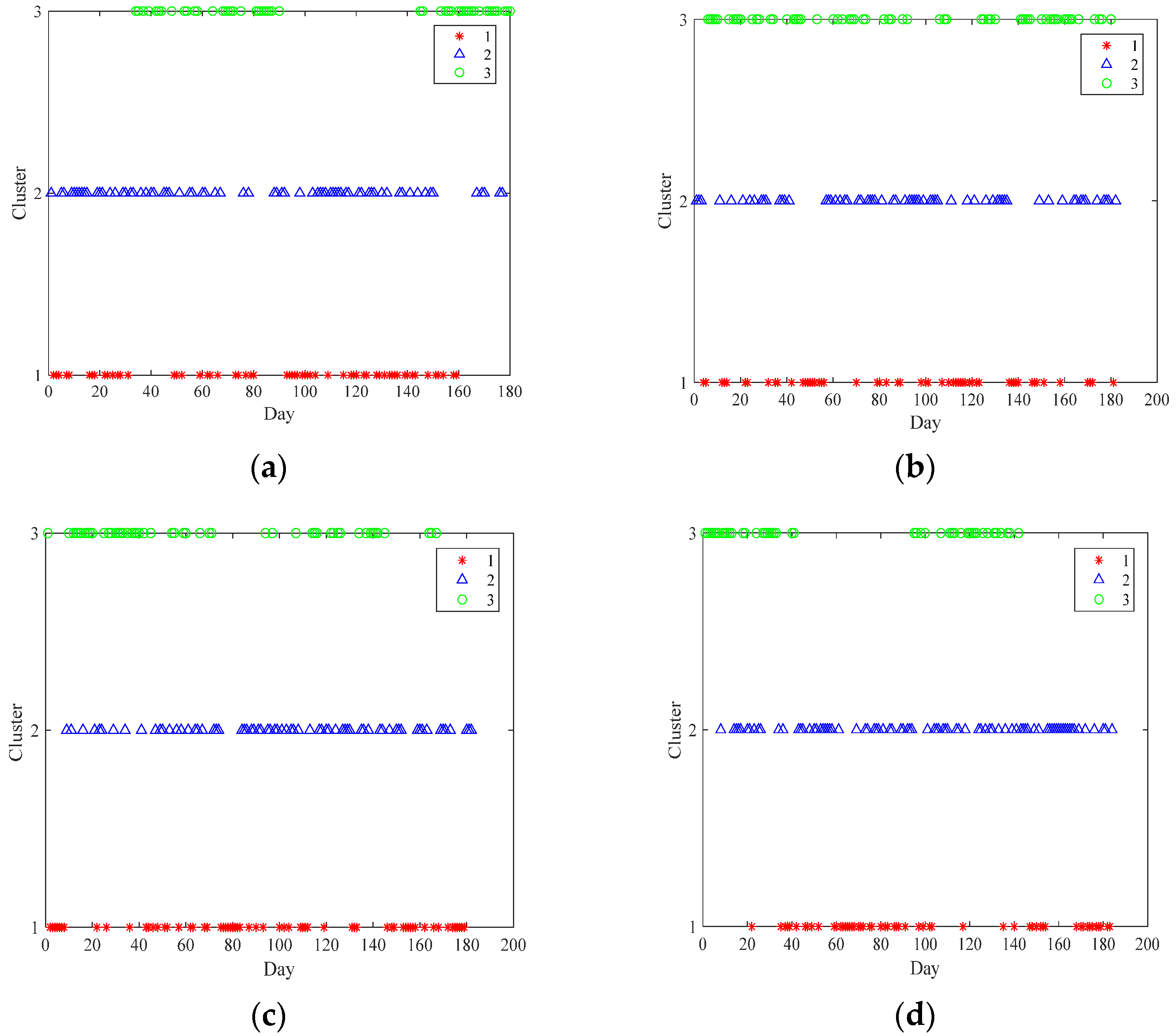
This paper aims to predict short-term solar radiation through a comprehensive application of machine learning techniques. Firstly, the missing values are recovered via the means of matrix completion with low-rank structure. Robust principal component analysis, a method of strong robustness to large spare noise, is employed to denoise the recovered data. Next, solar radiation data after denoising is clustered by fusing sparse subspace representation and k-nearest-neighbor. Subsequently, four artificial neural network models are used to forecast, and thus a kind of hybrid model for short-term solar radiation prediction is proposed.

The main structure of the paper is organized as follows. Section 2 describes the experimental dataset and methods. Machine learning techniques for data preprocessing are introduced in Section 3. Section 4 presents several machine learning techniques for forecasting solar radiation. In Section 5, the experiments are carried out, and a comparison of experimental results is provided. Section 6 draws conclusions.

2. Materials and Methods

2.1. Dataset

The global horizontal irradiation data was collected at a PV power plant in Jiangsu in China. The installed capacity of the power plant was nearly 1.1 megawatts-peak (MWP). The acquired data were recorded every 5 min and the period was from 2018 to 2019, but the dates of 25 and 26 September in 2019 were not considered, due to an error in collection. There were in totally 288 recordings each day. A small amount of abnormal data was generated due to equipment or operation failures, and these unreasonable recordings were regarded as missing entries in this paper. Figure 2 illustrates the solar radiation in 2018 and 2019, respectively, where the blue trend represents lower solar radiation intensity and the yellow trend represents higher solar radiation intensity. It can be seen from two the subfigures that solar radiation is mainly concentrated from 7 a.m. to 6 p.m. each day, and the solar radiation intensity is generally stronger from 12 a.m. to 3 p.m.

We separated all solar radiation data according to the four seasons: spring, summer, autumn and winter. In total, spring owns 180 days including January, February and March. In summer, there are 182 days in April, May and June. There are 182 days in July, August and September in autumn. Winter has 184 days in October, November and December. Figure 3 further illustrates the solar radiation intensity of the four seasons in 2018. In that year, the average daily maximum value of solar radiation intensity of spring is 592.64 Wh/m². In summer and autumn, the average daily maximum solar radiation intensity is 879.88 Wh/m² and 949.67 Wh/m², respectively. Compared with the other seasons, the average daily maximum solar radiation intensity in winter is only 549.33 Wh/m².

By observing Figure 2 and Figure 3, we can see that these data show no obvious trend or seasonality. What is more, the data are relatively complicated and there are many missing elements. If the original data were directly utilized to perform forecasting, the prediction results would probably have a large error, which would affect the normal operation of the PV power grid. According to the above data characteristics, it is essential to choose the appropriate data processing method. For obtaining higher data quality, we need to recover the missing entries and denoise the completed data. Subsequently, cluster analysis is adopted to reduce the complexity of data. The data of each cluster are chosen to make predictions separately, which can improve the prediction efficiency and accuracy to some extent.

2.2. Construction of the Hybrid Model

The hybrid model presented in this paper can be divided into the following two parts. The first part adopts machine learning methods including matrix completion, RPCA (robust principal component analysis) and cluster analysis to preprocess the original data. In the second part, the prediction is carried out by making use of the neural network in a machine learning method such as the BP neural network, radial basis function, extreme learning machine and long short-term memory.

Figure 4 shows the flow chart of the proposed hybrid model. The main process of data preprocessing includes the recovery of missing data through matrix completion, denoising of the completed dataset, and spectral clustering based on the combination of sparse subspace representation and k-nearest-neighbor. By integrating the neural network models, a short-term solar radiation prediction model is accomplished.

3. Machine Learning Techniques for Data Preprocessing

This section will introduce three unsupervised machine learning methods to preprocess solar radiation data. Firstly, a matrix completion method is utilized to recover the missing data. Then, robust principal component analysis (RPCA) is employed to denoise the completed data. Ultimately, a spectral clustering method based on the fusion of k-nearest-neighbor and sparse subspace representation is proposed to perform cluster analysis on the denoised data.

3.1. Data Completion and Denoising

3.1.1. Matrix Completion

Let ${\mathit{z}}_i\in {\Re }^{m\times 1}$ be an irradiation measure vector in the i-th day, $i=1,2,\dots ,n$. These n samples can be expressed as the matrix $\mathit{Z}=\left({\mathit{z}}_1,{\mathit{z}}_2,\dots ,{\mathit{z}}_n\right)$. For any real matrix $\mathit{Z}=(z_{ij}{)}_{m\times n}$, its nuclear norm is defined as ${\Vert \mathit{Z}\Vert }_{\ast }={\displaystyle {\sum }_{j=1}^{\min (m,n)}{\mathsf{\sigma }}_j}$, where ${\mathsf{\sigma }}_j$ is the j-th largest singular value of Z. To indicate all missing entries of Z, an index set $\mathsf{\Omega }\subset \{1,2,\dots ,m\}\times \{1,2,\dots ,n\}$ is firstly introduced. Subsequently, a projection operator of $P_{\mathsf{\Omega }}(·)$: ${\Re }^{m\times n}\to {\Re }^{m\times n}$ is defined as follows. If $(i,j)\in \Omega$, then $P_{\mathsf{\Omega }}(z_{ij})=z_{ij}$; otherwise, $P_{\mathsf{\Omega }}(z_{ij})=0$.

With regard to solar radiation, n samples can be roughly divided into several groups. Therefore, Z is approximately low-rank when n is relatively large. In the presence of missing elements, the recovery technique by the aid of the low-rank structure is called matrix completion [36,37]. Matrix completion is initially described as an affine rank minimization problem. However, due to the non-convexity and discontinuity of the rank function, it is intractable to address this problem. To this end, the aforementioned optimization model can be convexly relaxed into the matrix nuclear norm minimization [38,39]. Thus, the mathematical model of matrix completion is formulated as follows:

$$\underset{\tilde{\mathit{Z}}}{\min }{\Vert \tilde{\mathit{Z}}\Vert }_{\ast }\mathrm{s}.\mathrm{t}.{\mathrm{P}}_{\mathsf{\Omega }}(\tilde{\mathit{Z}})={\mathrm{P}}_{\mathsf{\Omega }}(\mathit{Z})$$

(1)

where $\tilde{\mathit{Z}}$ is the completed matrix. The optimal solution of the above minimization is also denoted as $\tilde{\mathit{Z}}$ to avoid abuse of symbols.

3.1.2. Robust Principal Component Analysis

Observing Figure 1 and Figure 2, we find that the solar radiation data is contaminated by some large sparse noise, which is detrimental for forecasting the future trend. For a low-rank data matrix corrupted by small dense noise, principal component analysis (PCA) can effectively perform dimension reduction, noise elimination, and feature extraction [39]. However, generally speaking, PCA does not work well when the studied dataset is superposed by large sparse noise or outliers. Hence, research on the robustness of PCA has always been the main focus of attention.

The emerging robust principal component analysis (RPCA) decomposes a matrix into the sum of a low-rank matrix and a sparse noise matrix, and the principal component pursuit is proposed to obtain the optimal decomposition [40]. This robust version of PCA can accurately recover the low rank component and the sparse noise under some conditions [41,42]. Formally, RPCA is modeled as follow:

$$\underset{\mathit{A},\mathit{E}}{\min }{\Vert \mathit{A}\Vert }_{*}+\lambda {\Vert \mathit{E}\Vert }_1,\mathrm{s}.\mathrm{t}.\tilde{\mathit{Z}}=\mathit{A}+\mathit{E}$$

(2)

where $\mathit{A}$ is the low-rank component, E is the sparse noise matrix, $\lambda >0$ balances the low rankness and the sparsity, ${\Vert ·\Vert }_1$ is the $l_1$-norm of a matrix (i.e., the sum of absolute values of all elements). The alternating direction method of multipliers is frequently used to solve the nuclear norm minimization (1) and (2). The optimal solution of the above minimization is denoted as $\tilde{\mathit{A}}$.

3.2. Data Cluster Analysis

3.2.1. k-Nearest-Neighbor

Cluster analysis refers to the process of dividing a given data set into several groups based on the similarity or the distance between two samples without prior information, and it is beneficial to further explore and mine the essence of the data [43]. Spectral clustering is a popular clustering method based on graph theory. The cluster task is achieved by clustering the eigenvectors of the Laplacian matrix for the sample set [44]. It can be explained that the core of spectral clustering is to map the points from high-dimensional space to low-dimensional space, and some clustering algorithms are used in low-dimensional space. A similarity matrix is an important index in spectral clustering, and it is constructed according to the distance metric among all points [45]. In the spectral clustering algorithm, the similarity between two points with a short distance is relatively high, otherwise the similarity is relatively low. The similarity matrix can be built up through three ways: ε-neighborhood graph, k-nearest-neighbor graph and fully connected graph [46]. Among these three manners, ε-neighborhood graph and fully connected graph probably lose more information, which leads to less accurate results. In contrast, the k-nearest-neighbor graph generally has a precise calculation result. Meanwhile, it is simple and easy to realize [47].

The first step of spectral clustering is to establish a weighted graph $G=(\nu ,\epsilon )$, where $\nu$ is the set of n nodes and $\epsilon$ is a collection of edges among nodes. Let $\tilde{\mathit{A}}=\left({\tilde{\mathit{a}}}_1,{\tilde{\mathit{a}}}_2,\dots {\tilde{\mathit{a}}}_n\right)$. The i-th node corresponds to the processed observation vector ${\tilde{\mathit{a}}}_i$. Constructing the similarity graph is the most crucial task for spectral clustering. Among the existing approaches, the k-nearest-neighbor graph is generally recommended as the first choice. Next, we introduce the construction process of the similarity matrix based on the k-nearest-neighbor graph.

In a manifold space, there exists an approximate liner relationship among the adjacent points. Under this circumstance, the distance between ${\tilde{\mathit{a}}}_i$ and ${\tilde{\mathit{a}}}_j$ is calculated by $d_{ij}={\Vert {\tilde{\mathit{a}}}_i-{\tilde{\mathit{a}}}_j\Vert }_2$, where ${\Vert ·\Vert }_2$ is the $l_2$-norm of a vector. Given ${\tilde{\mathit{a}}}_i$, we first compute $n-1$ distances $\left\{d_{i1},d_{i2},\dots ,d_{i,i-1},d_{i,i+1},\dots ,d_{in}\right\}$ and then sort them by the increasing order. Therefore, k nearest neighbors of ${\tilde{\mathit{a}}}_i$ can be found according to k smallest distances. On this basis, we build up a similarity graph G: if ${\tilde{\mathit{a}}}_i$ is one of k nearest neighbors for ${\tilde{\mathit{a}}}_i$ or ${\tilde{\mathit{a}}}_j$ is one of k-nearest-neighbors for ${\tilde{\mathit{a}}}_j$, then an edge is added between the i-th and the j-th nodes and the weight ${\mathit{s}}_{ij}$ is set to 1; otherwise, no edge exists and ${\mathit{s}}_{ij}=0$. Eventually, the similarity matrix $\mathit{S}={(s_{ij})}_{n\times n}$ is obtained and it is symmetrized by $s_{ij}\leftarrow \max \left\{s_{ij},s_{ji}\right\}$.

3.2.2. Sparse Subspace Representation

As a sparse learning method, sparse subspace representation is another manner to construct the similarity matrix in spectral clustering. Generally speaking, a high-dimensional dataset is distributed in the union of several low-dimensional subspaces. Hence, the representation of high-dimensional data is characterized by the sparseness [48,49,50].

It is supposed that the dataset locates in the union of several disjoint linear subspaces. The purpose of cluster analysis is to recognize and separate these subspaces. If $\tilde{\mathit{A}}$ is noise-free and there exist sufficient samples or points in each subspace, then the i-th sample can be expressed by the linear combination of the remainder, $i=1,2,3,\dots ,n$. Thus, it holds that

$${\tilde{\mathit{a}}}_i=v_{1i}{\tilde{\mathit{a}}}_1+v_{2i}{\tilde{\mathit{a}}}_2+\dots +v_{i-1,i}{\tilde{\mathit{a}}}_{i-1}+v_{i+1,i}{\tilde{\mathit{a}}}_{i+1}+\dots +v_{ni}{\tilde{\mathit{a}}}_n$$

(3)

where $v_{ji}\left(j\ne i\right)$ is the linear representation coefficient of the j-th sample. Let ${\mathit{v}}_i={\left(v_{1i},v_{2i},\dots ,v_{ni}\right)}^{\mathrm{T}}$, where $v_{ii}=0$. If $v_{ji}$ is large in the sense of absolute value, the i-th and the j-th samples probably have strong similarity.

Equation (3) can be written as ${\tilde{\mathit{a}}}_i=\tilde{\mathit{A}}{\mathit{v}}_i$. In detailed implementation, the optimal coefficient vector ${\mathit{v}}_i$ can be obtained by solving the following $l_p$-norm optimization problem:

$$\underset{{\mathit{v}}_i}{\min }{\Vert {\mathit{v}}_i\Vert }_p,\mathrm{s}.\mathrm{t}.{\tilde{\mathit{a}}}_i=\tilde{\mathit{A}}{\mathit{v}}_i$$

(4)

The value of p is commonly set to 1 or 2. The samples matrix $\tilde{\mathit{A}}$ is frequently corrupted by the superposition of small dense noise and large sparse noise. Under this circumstance, the vector ${\tilde{\mathit{a}}}_i$ is rewritten as:

$${\tilde{\mathit{a}}}_i=\tilde{\mathit{A}}{\mathit{v}}_i+{\mathit{e}}_i+{\mathit{o}}_i$$

(5)

where ${\mathit{e}}_i$ is a large sparse noise vector and the noise vector ${\mathit{o}}_i$ is dense. We assume that ${\mathit{e}}_i$ follows a Gaussian distribution, both ${\mathit{e}}_i$ and ${\mathit{v}}_i$ obey two multivariate Laplacian distributions. By applying the maximum likelihood estimation, we formulate an optimization problem:

$$\underset{{\mathit{v}}_i,{\mathit{e}}_i,{\mathit{o}}_i}{\min }{\Vert v_i\Vert }_1+{\lambda }_1{\Vert {\mathit{e}}_i\Vert }_1+{\lambda }_2{\Vert \tilde{\mathit{a}}\Vert }_2^2/2,\mathrm{s}.\mathrm{t}.{\tilde{\mathit{a}}}_i=\tilde{\mathit{A}}{\mathit{v}}_i+{\mathit{e}}_i+{\mathit{o}}_i$$

(6)

where ${\lambda }_1\ge 0$ and ${\lambda }_2\ge 0$ are two regularization parameters. Hence, the minimization problem (6), also named as sparse subspace representation, is more robust than problem (4) in dealing with dense and large sparse noise.

3.2.3. Spectral Clustering via Fusing k-Nearest-Neighbor and Sparse Subspace Representation

The main disadvantage of k-nearest-neighbor is that it does not use global information, which possibly leads to the less robustness to data noise. As an exceedingly robust method, the sparse subspace representation not only transmits valuable information in the classification task, but also makes use of the overall context information to provide a data adaptive neighborhood [46]. However, a drawback of the sparse subspace representation is that two samples with a large Euclidean distance may be classified into the same cluster. For this propose, this paper provides a spectral clustering fusing the advantages of k-nearest-neighbor and sparse subspace representation, and applies it to the cluster analysis on solar radiation.

Let ${\mathit{W}}_{\mathrm{k}}$ be the similarity matrix constructed by the k-nearest-neighbor and ${\mathit{W}}_{\mathrm{s}}$ be the similarity matrix obtained by sparse subspace representation. In consideration of their construction principles, both ${\mathit{W}}_{\mathrm{k}}$ and ${\mathit{W}}_{\mathrm{s}}$ are sparse and symmetric. We propose a weighted similarity matrix defined by the convex combination between ${\mathit{W}}_{\mathrm{k}}$ and ${\mathit{W}}_{\mathrm{s}}$:

$$\mathit{W}=\gamma {\mathit{W}}_{\mathrm{k}}+\left(1-\gamma \right){\mathit{W}}_{\mathrm{s}}$$

(7)

where $\gamma \in$ [0,1] is the trade-off parameter. When $\gamma =0$, the similarity matrix is constructed by sparse subspace representation. In addition, $\gamma$ = 1 means that the similarity matrix is formed by the k-nearest-neighbor.

Based on the resulting similarity matrix W, we divide the dataset matrix $\tilde{\mathit{A}}$ into s clusters via the spectral clustering method. The following lists the implementation procedure of spectral clustering. Firstly, a diagonal matrix D is calculated, whose diagonal elements are constructed by the sum of each row in W. Then the Laplacian matrix is computed as $\mathit{L}={\mathit{D}}^{-1/2}\mathit{W}{\mathit{D}}^{-1/2}$. Next, the eigen decomposition is performed on L and s mutually orthogonal unit eigenvectors ${\{{\mathit{a}}_i^v\in {\Re }^{m\times 1}\}}_{i=1}^s$ corresponding to s largest eigenvalues are acquired. Denote ${\mathit{A}}^v=\left({\mathit{a}}_1^v,\dots ,{\mathit{a}}_s^v\right)\in {\Re }^{m\times s}$. Each row of ${\mathit{A}}^v$ is further transformed into unit vectors in the sense of $l_2$-norm and the normalized matrix is indicated by ${\tilde{\mathit{A}}}^v$. Finally, each row of $\tilde{\mathit{A}}$ is regarded as a sample and m samples are partitioned into s clusters by k-means clustering. Compared with only using k-nearest-neighbor or sparse subspace representation, the proposed spectral clustering can maintain a stronger stability and robustness.

4. Machine Learning Techniques for Forecasting

Given input–output paired training samples ${\left\{({\mathit{x}}_i,{\mathit{y}}_i)\right\}}_{i=1}^N$, we consider the supervised learning task of seeking for an approximate function $\mathit{y}=f(\mathit{x})$, where ${\mathit{x}}_i\in {\Re }^{D_1\times 1}$ is the input vector and ${\mathit{y}}_i\in {\Re }^{D_2\times 1}$ is the output vector. To learn the function relationship between the input and the output, this section will introduce four supervised machine learning methods, namely, BP neural networks, radial basis function networks, extreme learning machines and long-short term memory models.

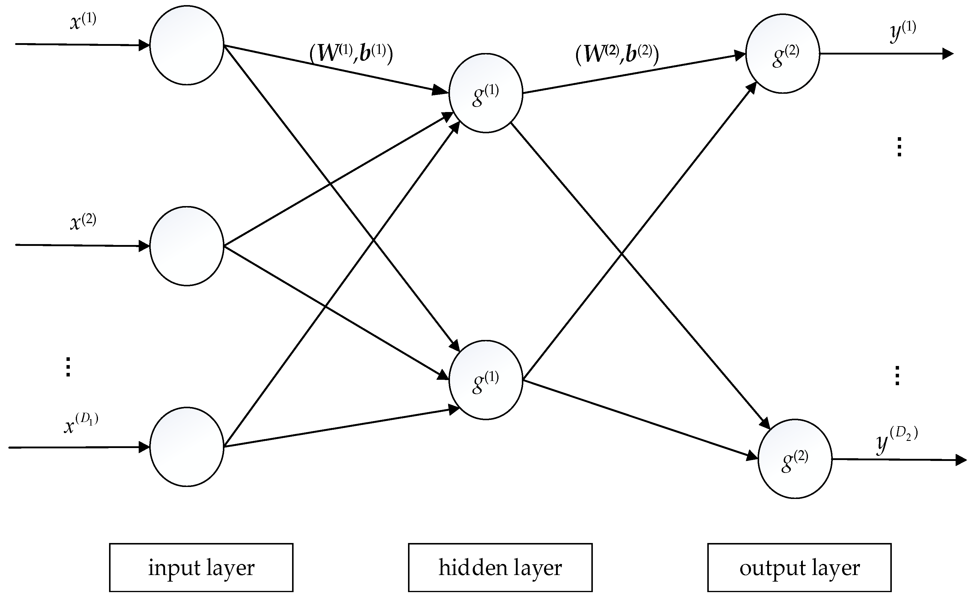
4.1. BP Neural Networks

Neural networks construct the functional form of $\mathit{y}=f(\mathit{x})$ from the viewpoint of a network model [26,51]. For an input vector $\mathit{x}={\left(x^{(1)},x^{(2)},\dots ,x^{(D_1)}\right)}^{\mathrm{T}}$, a feedforward network with K-1 hidden layers can be expressed by:

$$\mathit{y}\approx f_{\mathrm{BP}}(\mathit{x})=g^{(K)}\left({\mathit{W}}^{(K)}{g}^{(K-1)}\left({\mathit{W}}^{(K-1)}{g}^{(K-2)}\left(\dots g^{(1)}({\mathit{W}}^{(1)}\mathit{x}+{\mathit{b}}^{(1)})\dots \right)+{\mathit{b}}^{(K-1)}\right)+{\mathit{b}}^{(K)}\right)$$

(8)

where ${\mathit{W}}^{(k)}\in {\Re }^{d_k\times d_{k-1}}$ is the weights matrix in the k-th hidden layer, ${\mathit{b}}^{(k)}\in {\Re }^{d_k\times 1}$ is the corresponding bias vector, $g^{(k)}(\cdot )$ is the nonlinear activation function adopted in the k-th hidden layer, $d_0=D_1$ and $d_K=D_2$.

Denote the model parameters set by $\mathit{\theta }={\left\{{\mathit{W}}^{(k)},{\mathit{b}}^{(k)}\right\}}_{k=1}^K$. By training the network according to all training samples, the optimal network parameters $\mathit{\theta }$ can be obtained. For this purpose, we minimize the following error function:

$$E(\mathit{\theta })=\frac{1}{2}{\displaystyle \sum _{i=1}^N{\Vert f_{\mathrm{BP}}({\mathit{x}}_i)-{\mathit{y}}_i\Vert }_2^2}$$

(9)

The simplest and the most effective approach is the gradient descent, and the update formulation is

$$\mathit{\theta }\leftarrow \mathit{\theta }-\eta \nabla E(\mathit{\theta })$$

(10)

where $\nabla E(\mathit{\theta })$ is the gradient of $E(\mathit{\theta })$ with respect to $\mathit{\theta }$, and the step size $\eta$ is called the learning rate.

Each parameter updating step consists of two stages. The first stage evaluates the derivatives of the error function with respect to the weight matrices and the bias vectors. The backpropagation technique propagates errors backwards through the network and it has become a computationally efficient method for evaluating the derivatives. The derivatives are employed to adjust all parameters in the second stage. Hence, the multilayer perceptron is also called a back-propagation (BP) neural network. Figure 5 depicts the topological structure of a BP neural network with one hidden layer. In detailed implementation, mini-batch gradient descent is usually utilized to update parameters to reduce the computation burden.

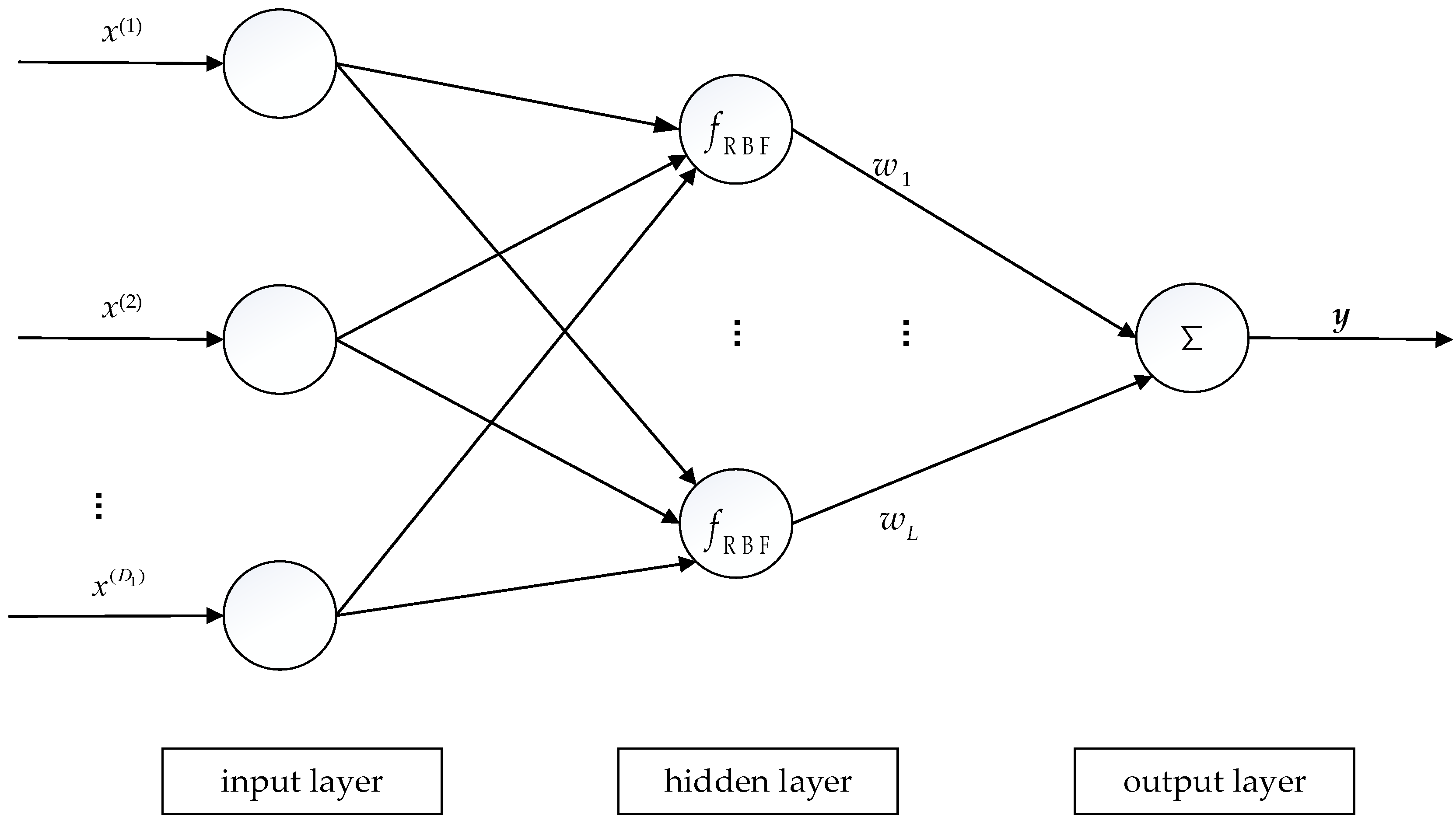
4.2. RBF Neural Networks

As a two-layer feedforward network, a radial basis function (RBF) neural network is composed of an input layer, a hidden layer and an output layer [27]. An RBF network is a special case of BP network, and the major difference lies in that the former uses a radial basis function as activation function instead of other functions, such as a sigmoid activation function. The sigmoid activation function forces the neurons to have a large input visible area [52]. In contrast, the activation function in an RBF network has a small input space region. Consequently, an RBF network needs more radial basis neurons. Moreover, an RBF network is mainly applied to the one-dimensional output case. Figure 6 plots the RBF neural network with the case $D_2=1$.

The commonly used radial basis function in an RBF neural network is the Gaussian function. Under this circumstance, the activation function for a given input feature $\mathit{x}$ can be expressed as

$$\mathsf{\phi }(\mathit{x};\mathit{u},\mathsf{\sigma })=\exp \left(-\frac{1}{2{\mathsf{\sigma }}^2}{\Vert \mathit{x}-\mathit{u}\Vert }^2\right)$$

(11)

where $\mathit{u}\in {\Re }^{D_1\times 1}$ and $\mathsf{\sigma }$ are the center and the standard deviation of the Gaussian function, respectively. The mathematical model of the RBF network with L hidden units can be written as

$$\mathit{y}\approx f_{\mathrm{RBF}}(\mathit{x};\mathit{\theta },\mathit{w})={\displaystyle \sum _{j=1}^L{w}_j}\mathsf{\phi }(\mathit{x};{\mathit{u}}_j,{\mathsf{\sigma }}_j)$$

(12)

where $\mathit{w}={(w_1,w_2,\dots ,w_L)}^{\mathrm{T}}$ is the weights vector connecting the hidden layer to the output layer, $\mathit{\theta }=\left\{\right({\mathit{u}}_j,{\mathsf{\sigma }}_j{\left)\right\}}_{j=1}^L$ is a set composed by L center vectors and L standard deviations.

Formally, the parameters of the RBF neural network can be obtained by minimizing the following errors:

$$\underset{\mathit{\theta },\mathit{w}}{\min }\frac{1}{2}{\displaystyle \sum _{i=1}^L{\left({\mathit{y}}_i-f_{\mathrm{RBF}}({\mathit{x}}_i;\mathit{\theta },\mathit{w})\right)}^2}$$

(13)

If $\mathit{\theta }$ is fixed, the optimal weights vector $\mathit{w}$ is calculated as

$$\mathit{w}\leftarrow {\mathit{\Phi }}^{†}\mathit{Y}$$

(14)

where $\mathit{Y}=({\mathit{y}}_1,{\mathit{y}}_2,\dots ,{\mathit{y}}_N{)}^{\mathrm{T}}$, the notation $†$ is the generalized inverse of a matrix, $\mathit{\Phi }={\left({\mathsf{\phi }}_{ij}\right)}_{N\times L}$ is the design matrix with ${\mathsf{\phi }}_{ij}=\mathsf{\phi }({\mathit{x}}_i;{\mathit{u}}_j,{\mathsf{\sigma }}_j)$. The parameters set can be determined by the gradient descent or cross-validation method. In practice, $\mathit{\theta }$ and $\mathit{w}$ can be updated alternately.

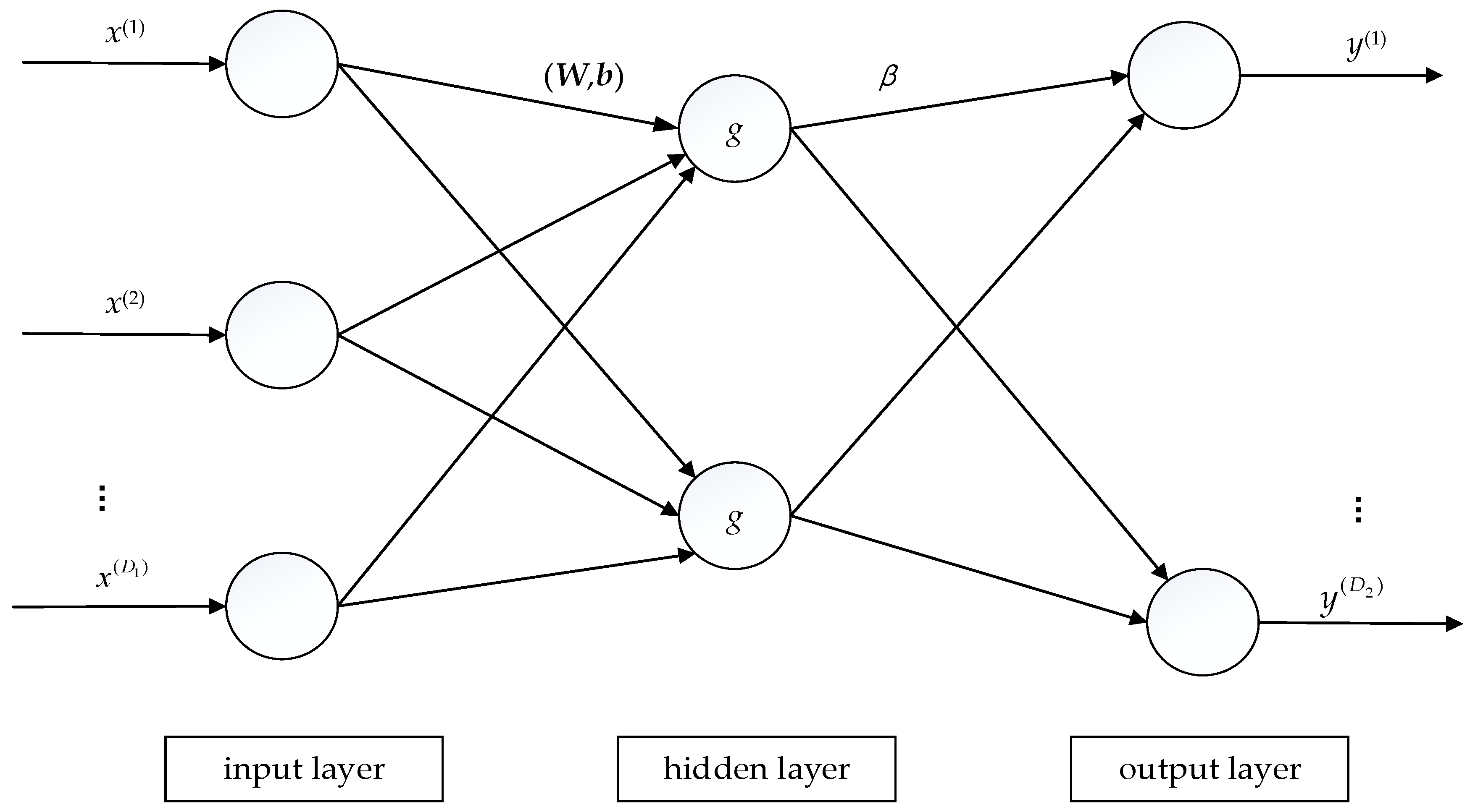
4.3. ELM Neural Networks

ELM generalizes single hidden layer feedforward networks [53,54,55]. For an input sample $\mathit{x}\in R^{D_1\times 1}$, ELM constructs a hidden layer with L nodes and the output of the i-th node is denoted by $h_i(\mathit{x})$, where $h_i(\mathit{x})$ is a nonlinear feature mapping. We can choose the output of all hidden layer nodes as follows:

$$\mathit{h}(\mathit{x};\mathit{W},\mathit{b})={\left(h_1(\mathit{x}),\dots ,h_L(\mathit{x})\right)}^{\mathrm{T}}=g(\mathit{W}x+\mathit{b})$$

(15)

where $\mathit{W}\in {\Re }^{L\times D_1}$ and $\mathit{b}\in {\Re }^{L\times 1}$ are the weight matrix and the bias vector in the hidden layer, respectively, and $g(\cdot )$ is the mapping function. Subsequently, the linear combination of ${\left\{h_i(\mathit{x})\right\}}_{i=1}^L$ is used as the resulting output of the prediction

$$\mathit{y}\approx f_{\mathrm{ELM}}(\mathit{x})={\left(\mathit{h}{(\mathit{x};\mathit{W},\mathit{b})}^{\mathrm{T}}\mathit{\beta }\right)}^{\mathrm{T}}$$

(16)

where $\mathit{\beta }\in {\Re }^{L\times D_2}$ is the output weight matrix. Figure 7 illustrates the diagram of an ELM neural network with one single hidden layer.

When all parameters $\left\{\mathit{W},\mathit{b},\mathit{\beta }\right\}$ are unknown, the above prediction function can be regarded as the combination of RBF networks and BP neural networks with only one hidden layer. To simplify the network model, extreme learning machines generate randomly the hidden node parameters $\left\{\mathit{W},\mathit{b}\right\}$ according to some probability distributions. In other words, W and b do not need to be trained explicitly, resulting in a remarkable efficiency.

Let $\mathit{H}={\left(\mathit{h}({\mathit{x}}_1;\mathit{W},\mathit{b}),\dots ,\mathit{h}({\mathit{x}}_N;\mathit{W},\mathit{b})\right)}^{\mathrm{T}}$, $\mathit{Y}={\left({\mathit{y}}_1,\dots ,{\mathit{y}}_N\right)}^{\mathrm{T}}$. The weights matrix $\mathit{\beta }$ connecting the hidden layer and the output layer can be solved by minimizing the squared error loss:

$$E(\mathit{\beta })=\frac{1}{2}{\displaystyle \sum _{i=1}^N{\Vert f_{\mathrm{ELM}}({\mathit{x}}_i)-{\mathit{y}}_i\Vert }^2}=\frac{1}{2}{\Vert \mathit{H}\beta -\mathit{Y}\Vert }_{\mathrm{F}}^2$$

(17)

where ${\Vert \cdot \Vert }_{\mathrm{F}}$ is the Frobenius norm of one matrix.

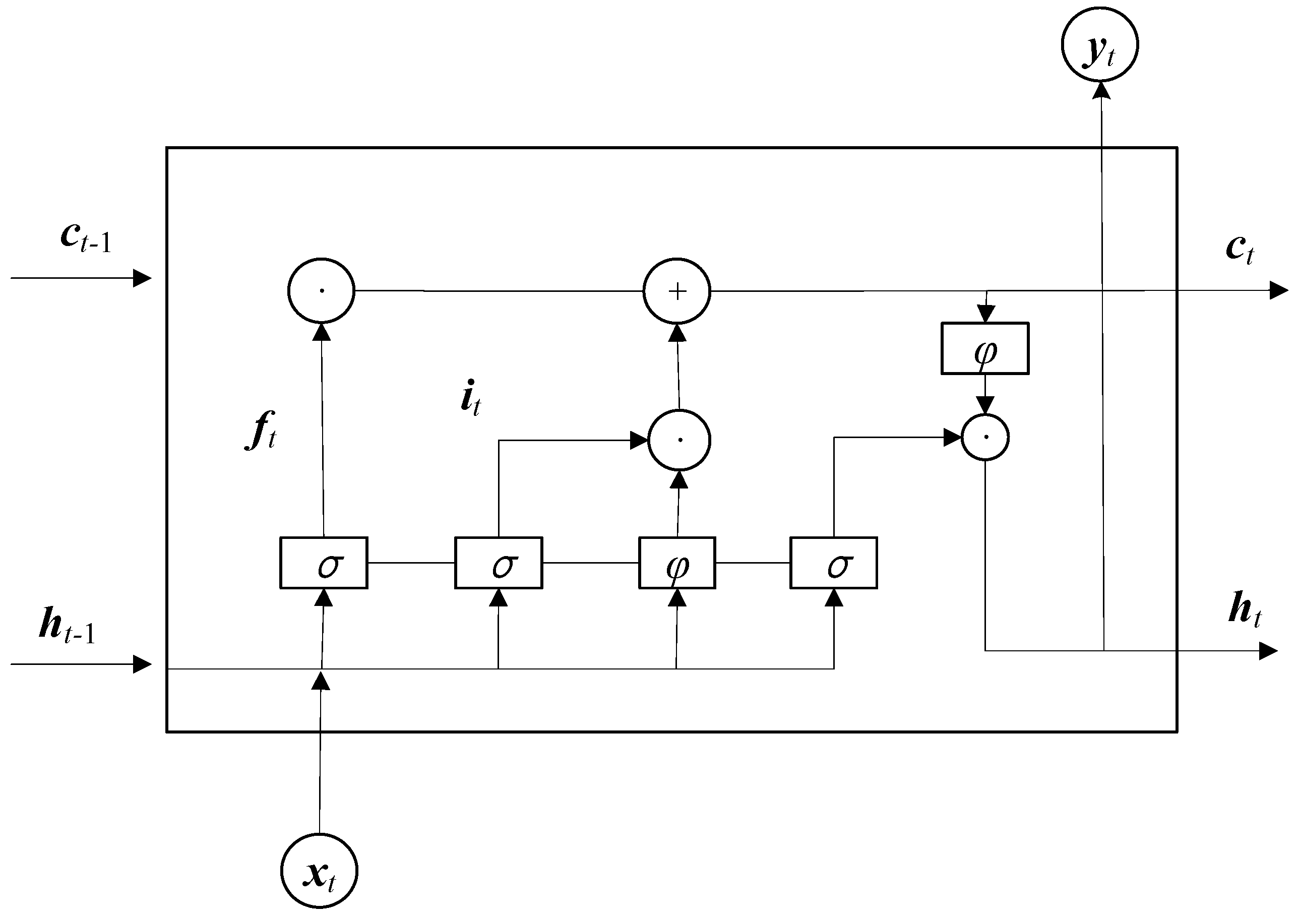
4.4. LSTM Neural Networks

As a special recurrent neural network (RNN), long short-term memory (LSTM) is suitable for processing and predicting important events with relatively long intervals and delays in the time series [56,57]. LSTM can alleviate the phenomenon of gradient disappearance in the structure of RNN [58]. As the result of a powerful representation ability, LSTM utilizes a complex nonlinear unit to construct larger deep neural networks.

LSTM controls long and short-term memory through gates and cell states [10]. As shown in Figure 8, the neurons in LSTM include input gate i, forget gate f, cell state c, output gate y. Among them, three gates are calculated as follows:

$${\mathit{i}}_t=\mathsf{\sigma }({\mathit{W}}_i·[{\mathit{h}}_{t-1},{\mathit{x}}_t]+{\mathit{b}}_i)$$

(18)

$${\mathit{f}}_t=\mathsf{\sigma }({\mathit{W}}_f·[{\mathit{h}}_{t-1},{\mathit{x}}_t]+{\mathit{b}}_f)$$

(19)

$${\mathit{y}}_t=\mathsf{\sigma }({\mathit{W}}_y·[{\mathit{h}}_{t-1},{\mathit{x}}_t]+{\mathit{b}}_y)$$

(20)

where ${\mathit{b}}_i$, ${\mathit{b}}_f$, ${\mathit{b}}_y$ are bias terms, ${\mathit{W}}_i$, ${\mathit{W}}_f$, ${\mathit{W}}_y$ are respectively the weight matrices of three gates, and $\mathsf{\sigma }$ is the sigmoid activation function. In Equation (18), ${\mathit{W}}_i·[{\mathit{h}}_{t-1},{\mathit{x}}_t]$ indicates ${\mathit{W}}_{i1}{\mathit{h}}_{t-1}+{\mathit{W}}_{i2}{\mathit{x}}_t$ where ${\mathit{W}}_i=\left({\mathit{W}}_{i1},{\mathit{W}}_{i2}\right)$. At time t, the update formula of cell state is:

$${\mathit{c}}_t={\mathit{f}}_t\odot {\mathit{c}}_{t-1}+{\mathit{i}}_t\odot {\tilde{\mathit{c}}}_t$$

(21)

where $\odot$ is the Hadamard product and ${\tilde{\mathit{c}}}_t$ is the candidate cell state. Let ${\mathit{b}}_c$ and $\mathit{W}$ be respectively the bias vector and the weight matrix of the candidate cell gate. Then ${\tilde{\mathit{c}}}_t$ is computed as:

$${\tilde{\mathit{c}}}_t=\phi ({\mathit{W}}_c·[{\mathit{h}}_{t-1},{\mathit{x}}_t]+{\mathit{b}}_c)$$

(22)

where the activation function $\phi$ is usually chosen as the hyperbolic tangent. At last, the hidden vector is updated:

$${\mathit{h}}_t={\mathit{y}}_t\odot \phi ({\mathit{c}}_t)$$

(23)

For the input information ${\mathit{x}}_t$, Equation (22) calculates the candidate cell state ${\tilde{\mathit{c}}}_t$ at time t by ${\mathit{h}}_{t-1}$ and ${\mathit{x}}_t$. Equation (21) combines the input gate and the forgetting gate to update the cell state ${\mathit{c}}_t$ at time t. Equation (23) calculates the hidden layer information at time t. Through the combination with gate control units, the LSTM network achieves the purpose of memorizing long- and short-term information of time series data by continuously updating the cell state at each moment.

5. Experimental Results

5.1. Model Implementation

The solar radiation observation dataset was collected from a certain part of Jiangsu Province in 2018 and 2019. It can be formed into the matrix $\mathit{Z}={(z_{ij})}_{m\times n}$, where m = 288 is the total number of recordings per day, and n = 728 is the number of days for that selected two years.

First of all, in view of the incompleteness of these solar radiation data, the matrix completion method is utilized to infer the missing elements. This procedure can further refine and calibrate these data. In 2018, 363 days are considered and there are 92 pieces of missing data in total. There are 365 days in 2019, and 28 pieces of data are missing. Taking 11 January 2018 as an example, there are 279 recordings and 9 missing values, and Figure 9 illustrates the completed data in that day. In this figure, the blue stars represent the observed values and the red filled circles are the recovered values by matrix completion. As we can see, the matrix completion has a good recovery performance in that day. In summary, 104,544 and 105,120 recording values, respectively, are obtained after completion.

The recovered solar radiation data are further divided into four parts according to the four seasons, and RPCA is employed to denoise the completed data of each season. Figure 10 shows the solar radiation waveforms of 20 non-repeated days before and after denoising for each season, and different colors indicate different days. It can be seen that the solar radiation is zero before 6 a.m. and after 7 p.m. in most cases. It is especially important that the denoised data are convenient for us to grasp the real trend of the variation in solar radiation data, which is conducive to a better prediction of solar radiation.

As can be seen from Figure 2 and Figure 3, the differences of solar radiation intensity in the four seasons are particularly striking, and the sub-dataset of each season is disorganized without any seasonal characteristics and periodicity. For the solar radiation of each season, we utilize spectral clustering based on the fusion of k-nearest-neighbor and sparse subspace representation to divide all the days in each season into three clusters from the solar radiation intensity. In Figure 11, we cluster the radiation data of all days in each season into Cluster 1, Cluster 2 and Cluster 3 according to the solar radiation intensity from low to high. At the upper right of each subplot in Figure 11, the red asterisks, the blue hollow triangles and the green circles stand for Cluster 1, Cluster 2 and Cluster 3, respectively. Springs in Clusters 1, 2 and 3 have 60, 71 and 49 days, respectively, and summers have 55, 65 and 62 days. In autumn, there are 63, 68 and 51 days in the three clusters respectively, winters last 60, 71 and 49 days, respectively.

When neural networks are used for predictions, we choose the solar radiation between 7 a.m. and 6 p.m. every day as the effective input data in order to improve the calculation speed and ensure the validity of the data. To enhance the short-term prediction ability of the proposed model, the solar radiation every two consecutive hours is selected as the training sample to predict that of the next moment. For each season, the last five days of each cluster are employed to construct the test set for final evaluation, and the remaining days are harnessed to train the neural networks. Attention should be paid as over-fitting may occur in the training process of the neural network, that is, the training error is small, but the generalization error is large. Therefore, in the experiment, we use the regularization technique for BP, RBF and ELM, and the dropout strategy for LSTM to prevent overfitting.

5.2. Performance Analysis

In order to verify the effectiveness of the proposed models, this subsection compares four commonly used neural networks, i.e., BP neural networks, RBF neural networks, ELM neural networks, and LSTM neural networks. Two commonly used statistical indices, the root mean square error (RMSE) and the mean absolute error (MAE), are adopted for model validation to quantitatively evaluate the prediction performance. Their formulations are as follows:

$$RMSE=\sqrt{\frac{1}{N}{\displaystyle \sum _{i=1}^N{\Vert {\widehat{\mathit{y}}}_i-{\mathit{y}}_i\Vert }_2^2}}$$

(24)

$$MAE=\frac{1}{N}{\displaystyle \sum _{i=1}^N{\Vert {\widehat{\mathit{y}}}_i-{\mathit{y}}_i\Vert }_1}$$

(25)

where ${\mathit{y}}_i$ is the actual value of the output data, and ${\widehat{\mathit{y}}}_i$ is the corresponding predicted result.

Table 1. RMSE of solar radiation forecast errors in spring.

without Clustering			with Clustering
		Cluster 1	Cluster 2	Cluster 3	Average
BP	53.84	58.21	58.96	34.21	50.46
RBF	98.42	65.09	58.53	49.71	57.78
ELM	58.91	56.15	63.30	45.61	55.02
LSTM	226.26	76.78	56.08	145.23	92.70

,

Table 2. MAE of solar radiation forecast errors in spring.

without Clustering			with Clustering
		Cluster 1	Cluster 2	Cluster 3	Average
BP	35.93	41.81	45.87	22.28	36.65
RBF	65.44	50.90	45.58	36.64	44.37
ELM	42.01	39.80	46.53	35.77	40.70
LSTM	215.07	62.18	39.38	108.53	70.03

,

Table 3. RMSE of solar radiation forecast errors in summer.

without Clustering			with Clustering
		Cluster 1	Cluster 2	Cluster 3	Average
BP	51.96	62.82	11.14	68.39	47.45
RBF	119.66	76.71	12.47	83.58	57.59
ELM	62.84	64.65	11.65	74.68	50.33
LSTM	182.40	105.48	198.70	118.88	141.02

,

Table 4. MAE of solar radiation forecast errors in summer.

without Clustering			with Clustering
		Cluster 1	Cluster 2	Cluster 3	Average
BP	34.54	50.83	9.20	49.46	36.50
RBF	88.71	61.76	9.81	65.85	45.81
ELM	43.84	50.91	9.11	56.38	38.80
LSTM	182.42	60.71	57.80	93.82	70.78

,

Table 5. RMSE of solar radiation forecast errors in autumn.

without Clustering			with Clustering
		Cluster 1	Cluster 2	Cluster 3	Average
BP	47.11	39.61	64.62	27.65	43.96
RBF	105.10	45.05	62.96	9.81	39.27
ELM	64.77	66.09	13.92	73.06	51.02
LSTM	195.22	73.35	76.66	122.46	90.82

,

Table 6. MAE of solar radiation forecast errors in autumn.

without Clustering			with Clustering
		Cluster 1	Cluster 2	Cluster 3	Average
BP	28.33	27.95	43.09	16.02	29.02
RBF	64.20	50.90	45.58	36.63	44.37
ELM	42.01	39.80	46.53	35.77	40.70
LSTM	158.67	39.38	77.85	116.81	78.01

,

Table 7. RMSE of solar radiation forecast errors in winter.

without Clustering			with Clustering
		Cluster 1	Cluster 2	Cluster 3	Average
BP	34.66	23.95	54.90	10.51	29.79
RBF	62.16	28.14	54.28	17.18	33.20
ELM	46.89	31.66	62.30	14.68	36.21
LSTM	155.57	40.44	43.50	35.50	39.81

and

Table 8. MAE of solar radiation forecast errors in winter.

without Clustering			with Clustering
		Cluster 1	Cluster 2	Cluster 3	Average
BP	18.22	14.73	34.41	8.24	19.13
RBF	46.93	12.78	34.68	16.28	21.25
ELM	30.53	21.16	43.30	11.85	25.44
LSTM	147.43	26.23	32.21	26.00	27.14

list the prediction results of BP, RBF, ELM and LSTM in the situations of with or without clustering. For the case of without clustering, the RMSE/MAE values of 15 days in the test set of each season are reported. In the case of clustering, the prediction errors are recorded for the three clusters, respectively. The last columns in these tables give the average of the forecast results of the three clusters. Compared with the case of without clustering, the RMSE value of the BP network with clustering in the four seasons goes down respectively by 3.38, 4.51, 3.15 and 4.87, while MAE rises by 0.72, 1.96, 0.69 and 0.91, respectively. As for RBF, RMSE is respectively decreased by 40.64, 62.07, 65.83 and 28.96 and MAE is decreased by 21.07, 42.90, 19.83 and 25.18, respectively. When using ELM, RMSE is respectively reduced by 3.89, 12.51, 13.75 and 10.68 and MAE is reduced by 1.31, 5.04, 1.31 and 5.09. At last, RMSE of LSTM is improved respectively by 133.56, 41.38, 104.40 and 115.75, and MAE is improved by 145.04, 111.64, 80.6 and 120.29. The experimental results demonstrate that the performance of the four neural network models are enhanced via spectral clustering, which indicates that machine learning models are significative to improving the prediction results of short-time solar radiation.

Table 9. R² of solar radiation in spring.

without Clustering			with Clustering
		Cluster 1	Cluster 2	Cluster 3	Average
BP	0.8491	0.8732	0.9879	0.9699	0.9437
RBF	0.8318	0.8326	0.8763	0.9791	0.8960
ELM	0.8640	0.9294	0.8169	0.9779	0.9081
LSTM	0.8247	0.8129	0.8970	0.8060	0.8386

,

Table 10. R² of solar radiation in summer.

without Clustering			with Clustering
		Cluster 1	Cluster 2	Cluster 3	Average
BP	0.9500	0.9590	0.9981	0.9548	0.9706
RBF	0.9357	0.9294	0.9977	0.8169	0.9147
ELM	0.9538	0.9436	0.9405	0.9968	0.9603
LSTM	0.8576	0.8742	0.8176	0.8514	0.8477

,

Table 11. R² of solar radiation in autumn.

without Clustering			with Clustering
		Cluster 1	Cluster 2	Cluster 3	Average
BP	0.9733	0.9916	0.9055	0.9313	0.9428
RBF	0.9366	0.8777	0.8713	0.9888	0.9126
ELM	0.9437	0.9249	0.9916	0.8651	0.9272
LSTM	0.8554	0.8454	0.9196	0.7981	0.8543

and

Table 12. R² of solar radiation in winter.

without Clustering			with Clustering
		Cluster 1	Cluster 2	Cluster 3	Average
BP	0.9692	0.9364	0.8636	0.9982	0.9327
RBF	0.8769	0.9230	0.8687	0.9973	0.9299
ELM	0.9155	0.9558	0.8030	0.9970	0.9186
LSTM	0.8193	0.8309	0.8289	0.8877	0.8291

show the determination coefficient R² of solar radiation prediction by neural networks with and without clustering for four seasons. R² is a measure of how well the regression line represents the data, and the prediction models are more effective as R² approaches one. In contrast, in the case of without clustering, the R² of BP in the four seasons is respectively increased by 0.0946, 0.0206, −0.0305 and −0.0365 in the sense of average values. When applying RBF, R² is raised by 0.0642, −0.0210, −0.0240 and 0.0053. As for ELM, R² is improved by 0.0441, 0.0065, −0.0165 and 0.0031. With regard to LSTM, R² respectively went up by 0.0139, −0.0094, −0.0011 and 0.0098. The experimental results in these tables indicate that the proposed forecasting methods can significantly improve the prediction performance of short-term solar radiation in most cases.

Due to the added cluster analysis, the four data sets of spring, summer, autumn and winter are divided into three clusters with different irradiation intensities. At the same time, the similarity of samples in each cluster is relatively high in general. It can be seen from the aforementioned experimental results that the clustering strategy does improve the prediction accuracy. This observation can be explained by the reasoning that data preprocessing and sample partitions have a favorable impact on short-term solar radiation prediction. Ultimately, through analyzing the prediction results of various artificial neural networks, the proposed methods have indeed improved the prediction accuracy on the whole. These experimental results mean that the hybrid models of machine learning have advantages to some extent.

6. Conclusions and Outlook

This paper proposes a comprehensive application of machine learning techniques for short-term solar radiation prediction. Firstly, aiming at the missing entries in solar radiation data, a matrix completion method is used to recover them. Then we denoise the completed data by robust principal component analysis. The denoised data is clustered into low, medium and high intensity types via fusing sparse subspace representation and k-nearest-neighbor. Subsequently, four commonly used neural networks (BP, RBF, ELM and LSTM) are adopted to predict the solar radiation. In order to quantitatively verify the performance of the prediction model, the RMSE and MAE indicators are applied for model evaluation. The experimental results show that the hybrid model can improve the solar radiation predication accuracy.

In future research work, we will try to improve the model in the following respects to enhance its prediction ability. A multi-step forward prediction is necessary in practice, and it is urgent to develop the corresponding forecasting models by an ensemble of machine learning techniques and signal decomposition methods. In the procedure of establishing the prediction model, the input meteorological element used in this paper is only global horizontal irradiance. In fact, there are many other elements that affect solar radiation, such as the variation of daily temperature and precipitation. The influence of multiple elements on solar radiation will be considered and analyzed so as to improve the prediction ability of solar radiation. Furthermore, this paper only merges a few machine learning techniques into the forecast of solar radiation. In particular, deep learning models have a powerful representative ability and their further application in forecasting solar radiation will be very prospective.

References

1. Duffie, J.A.; Beckman, W.A.; Blair, N. Solar Engineering of Thermal Processes; John Wiley & Sons: Hoboken, NJ, USA, 2013; pp. 569–582. [Google Scholar]
2. Qazi, A.; Fayaz, H.; Wadi, A.; Raj, R.G.; Rahim, N.A.; Khan, W.A. The artificial neural network for solar radiation prediction and designing solar systems: A systematic literature review. J. Clean. Prod. 2015, 104, 1–12. [Google Scholar] [CrossRef]
3. Yagli, G.M.; Yang, D.; Srinivasan, D. Automatic hourly solar forecasting using machine learning models. Renew. Sustain. Energy Rev. 2019, 105, 487–498. [Google Scholar] [CrossRef]
4. Kleniewska, M.; Mitrowska, D.; Wasilewicz, M. Estimating daily global solar radiation with no meteorological data in Poland. Appl. Sci. 2020, 10, 778. [Google Scholar] [CrossRef] [Green Version]
5. Blal, M.; Seyfallah Khelifi, S.; Rachid Dabou, R. A prediction models for estimating global solar radiation and evaluation meteorological effect on solar radiation potential under several weather conditions at the surface of Adrar environment. Measurement 2020, 152, 107348. [Google Scholar] [CrossRef]
6. Ogliari, E.; Dolara, A.; Manzolini, G.; Leva, S. Physical and hybrid methods comparison for the day ahead PV output power forecast. Renew. Energy 2017, 113, 11–21. [Google Scholar] [CrossRef]
7. Başaran, K.; Bozyiğit, F.; Siano, P.; Taer, P.Y.; Kılınç, D. Systematic literature review of photovoltaic output power forecasting. IET Renew. Power Gener. 2021, 14, 3961–3973. [Google Scholar] [CrossRef]
8. Arif, B.M.; Hanafi, L.M. Physical reviews of solar radiation models for estimating global solar radiation in Indonesia. Energy Rep. 2020, 6, 1206–1211. [Google Scholar]
9. Paulescu, M.; Paulescu, E. Short-term forecasting of solar irradiance. Renew. Energy 2019, 143, 985–994. [Google Scholar] [CrossRef]
10. Huang, X.Q.; Li, Q.; Tai, Y.H.; Chen, Z.Q.; Zhang, J.; Shi, J.S.; Gao, B.X.; Liu, W.M. Hybrid deep neural model for hourly solar irradiance forecasting. Renew. Energy 2021, 171, 1041–1060. [Google Scholar] [CrossRef]
11. Nam, S.B.; Hur, J. A hybrid spatio-temporal forecasting of solar generating resources for grid integration. Energy 2019, 177, 503–510. [Google Scholar] [CrossRef]
12. Zhang, Y.; Li, Y.T.; Zhang, G.Y. Short-term wind power forecasting approach based on Seq2Seq model using NWP data. Energy 2020, 213, 118371. [Google Scholar] [CrossRef]
13. Zang, H.X.; Liu, L.; Sun, L.; Cheng, L.L.; Wei, Z.N.; Sun, G.Q. Short-term global horizontal irradiance forecasting based on a hybrid CNN-LSTM model with spatiotemporal correlations. Renew. Energy 2020, 160, 26–41. [Google Scholar] [CrossRef]
14. Schulz, B.; Ayari, M.E.; Lerch, S.; Baran, S. Post-processing numerical weather prediction ensembles for probabilistic solar irradiance forecasting. Sol. Energy 2021, 220, 1016–1031. [Google Scholar] [CrossRef]
15. Bakker, K.; Whan, K.; Knap, W.; Schmeits, M. Comparison of statistical post-processing methods for probabilistic NWP forecasts of solar radiation. Sol. Energy 2019, 191, 138–150. [Google Scholar] [CrossRef]
16. Verbois, H.; Huva, R.; Rusydi, A.; Walsh, W. Solar irradiance forecasting in the tropics using numerical weather prediction and statistical learning. Sol. Energy 2018, 162, 265–277. [Google Scholar] [CrossRef]
17. Chen, J.L.; He, L.; Yang, H.; Ma, M.H.; Chen, Q.; Wu, S.J.; Xiao, Z.L. Empirical models for estimating monthly global solar radiation: A most comprehensive review and comparative case study in China. Renew. Sustain. Energy Rev. 2019, 108, 91–111. [Google Scholar] [CrossRef]
18. Zheng, J.Q.; Zhang, H.R.; Dai, Y.H.; Wang, B.H.; Zheng, T.C.; Liao, Q.; Liang, Y.T.; Zhang, F.W.; Song, X. Time series prediction for output of multi-region solar power plants. Appl. Energy 2020, 257, 114001. [Google Scholar] [CrossRef]
19. David, M.; Ramahatana, F.; Trombe, P.J.; Lauret, P. Probabilistic forecasting of the solar irradiance with recursive ARMA and GARCH models. Sol. Energy 2016, 133, 55–72. [Google Scholar] [CrossRef] [Green Version]
20. Lee, J.H.; Wang, W.; Harrou, F.; Sun, Y. Reliable solar irradiance prediction using ensemble learning-based models: A comparative study. Energy Convers. Manag. 2020, 208, 112582. [Google Scholar] [CrossRef] [Green Version]
21. Voyant, C.; Notton, G.; Kalogirou, S. Machine learning methods for solar radiation forecasting: A review. Renew. Energy 2017, 105, 569–582. [Google Scholar] [CrossRef]
22. Gabriel, N.; Felipe, L.G.; Bressan Michael, B.; Andres, P. Machine learning for site-adaptation and solar radiation forecasting. Renew. Energy 2020, 167, 333–342. [Google Scholar]
23. Pang, Z.H.; Niu, F.X.; O’Neill, Z. Solar radiation prediction using recurrent neural network and artificial neural network: A case study with comparisons. Renew. Energy 2020, 156, 279–289. [Google Scholar] [CrossRef]
24. Ayodele, T.R.; Ogunjuyigbe, A.S.O.; Amedu, A.; Munda, J.L. Prediction of global solar irradiation using hybridized k-means and support vector regression algorithms. Renew. Energy Focus 2019, 29, 78–93. [Google Scholar] [CrossRef]
25. Panamtash, H.; Zhou, Q.; Hong, T.; Qu, Z.H.; Davis, K.O. A copula-based Bayesian method for probabilistic solar power forecasting. Sol. Energy 2020, 196, 336–345. [Google Scholar] [CrossRef]
26. Xue, X.H. Prediction of daily diffuse solar radiation using artificial neural networks. Int. J. Hydrog. Energy 2017, 42, 28214–28221. [Google Scholar] [CrossRef]
27. Alamin, Y.I.; Anaty, M.K.; Álvarez-Hervás, J.D.; Bouziane, K.; Pérez-García, M. Very short-term power forecasting of high concentrator photovoltaic power facility by implementing artificial neural network. Energies 2020, 13, 3493. [Google Scholar] [CrossRef]
28. Al-Dahidi, S.; Ayadi, O.; Adeeb, J.; Alrbai, M.; Qawasmeh, B.R. Extreme learning machines for solar photovoltaic power predictions. Energies 2018, 11, 2725. [Google Scholar] [CrossRef] [Green Version]
29. Huynh, A.N.L.; Deo, R.C.; An-Vo, D.A.; Ali, M. Near real-time global solar radiation forecasting at multiple time-step horizons using the long short-term memory network. Energies 2020, 13, 3517. [Google Scholar] [CrossRef]
30. Sharma, A.; Kakkar, A. Forecasting daily global solar irradiance generation using machine learning. Renew. Sustain. Energy Rev. 2018, 82, 2254–2269. [Google Scholar] [CrossRef]
31. Lan, H.; Zhang, C.; Hong, H.H.; He, Y.; Wen, S.L. Day-ahead spatiotemporal solar irradiation forecasting using frequency-based hybrid principal component analysis and neural network. Appl. Energy 2019, 247, 389–402. [Google Scholar] [CrossRef]
32. Hamid Mehdipour, S.; Tenreiro Machado, J.A. Cluster analysis of the large natural satellites in the solar system. Appl. Math. Model. 2021, 89, 1268–1278. [Google Scholar] [CrossRef]
33. Wang, K.J.; Qi, X.X.; Liu, H.D. A comparison of day-ahead photovoltaic power forecasting models based on deep learning neural network. Appl. Energy 2019, 251, 113315. [Google Scholar] [CrossRef]
34. Sun, S.L.; Wang, S.Y.; Zhang, G.W.; Zheng, J.L. A decomposition-clustering-ensemble learning approach for solar radiation forecasting. Sol. Energy 2018, 163, 189–199. [Google Scholar] [CrossRef]
35. Majumder, I.; Dash, P.K.; Bisoi, R. Variational mode decomposition based low rank robust kernel extreme learning machine for solar irradiation forecasting. Energy Convers. Manag. 2018, 171, 787–806. [Google Scholar] [CrossRef]
36. Mazumder, R.; Saldana, D.; Weng, H.L. Matrix completion with nonconvex regularization: Spectral operators and scalable algorithms. Stat. Comput. 2020, 30, 1113–1138. [Google Scholar] [CrossRef] [Green Version]
37. Shi, J.R.; Zheng, X.Y.; Zhou, S.S. Research progress in matrix completion algorithms. Comput. Sci. 2014, 41, 13–20. [Google Scholar]
38. Hu, Z.X.; Nie, F.P.; Wang, R.; Li, X.L. Low rank regularization: A review. Neural Netw. 2021, 136, 218–232. [Google Scholar] [CrossRef]
39. Shi, J.R.; Li, X.X. Meteorological data estimation based on matrix completion. Meteorol. Sci. Technol. 2019, 47, 420–425. [Google Scholar]
40. Shi, J.R.; Yang, W.; Zheng, X.Y. Robust generalized low rank approximations of matrices. Entopy 2015, 10, e0137028. [Google Scholar] [CrossRef]
41. Zhao, Q.; Meng, D.; Xu, Z. Robust principal component analysis with complex noise. In Proceedings of the 31st International Conference on Machine Learning ICML, Beijing, China, 21–26 June 2014; Volume 32, pp. 55–63. [Google Scholar]
42. Liu, L.; Gao, X.B.; Gao, Q.X.; Shao, L.; Han, J.G. Adaptive robust principal component analysis. Neural Netw. 2019, 119, 85–92. [Google Scholar] [CrossRef]
43. Dong, L.; Wang, L.J.; Khahro, S.F.; Gao, S.; Liao, X.Z. Wind power day-ahead prediction with cluster analysis of NWP. Renew. Sustain. Energy Rev. 2016, 60, 1206–1212. [Google Scholar] [CrossRef]
44. Luxburg, U.V. A tutorial on spectral clustering. Stat. Comput. 2004, 17, 395–416. [Google Scholar] [CrossRef]
45. Chen, W.F.; Feng, G.C. Spectral clustering with discriminant cuts. Knowl. Based Syst. 2012, 28, 27–37. [Google Scholar] [CrossRef]
46. Shi, J.R.; Yang, L. A climate classification of China through k-knearnst-neighbor and sparse subspace representation. J. Clim. 2020, 33, 243–262. [Google Scholar] [CrossRef]
47. Filippone, M.; Camastra, F.; Masulli, F.; Rovetta, S. A survey of kernel and spectral methods for clustering. Pattern Recognit. 2008, 41, 176–190. [Google Scholar] [CrossRef] [Green Version]
48. Wang, W.W.; Xiao-Ping, L.I.; Feng, X.C. A survey on sparse subspace clustering. Acta Autom. Sin. 2015, 41, 1373–1384. [Google Scholar]
49. Elhamifar, E.; Vidal, R. Sparse subspace clustering: Algorithm, theory, and applications. IEEE Trans. Pattern Anal. Mach. Intell. 2013, 35, 2765–2781. [Google Scholar] [CrossRef] [Green Version]
50. Zhou, Z.H.; Tian, B. Research on community detection of online social network members based on the sparse subspace clustering approach. Future Internet 2019, 11, 254. [Google Scholar] [CrossRef] [Green Version]
51. Wang, Z.; Wang, F.; Su, S. Solar Irradiance Short-Term Prediction Model Based on BP Neural Network. Energy Procedia 2011, 12, 488–494. [Google Scholar] [CrossRef] [Green Version]
52. Elsheikh, A.H.; Sharshir, S.W.; Elaziz, M.A.; Kabeel, A.E.; Wang, G.L.; Zhang, H.O. Modeling of solar energy systems using artificial neural network: A comprehensive review. Sol. Energy 2019, 180, 622–639. [Google Scholar] [CrossRef]
53. Huang, G.; Huang, G.B.; Song, S.J.; You, K.Y. Trends in extreme learning machines: A review. Neural Netw. 2015, 61, 32–48. [Google Scholar] [CrossRef]
54. Aybar-Ruiz, A.; Jiménez-Fernández, S.; Cornejo-Bueno, L.; Casanova-Mateo, C.; Sanz-Justo, J.; Salvador-González, P.; Salcedo-Sanz, S. A novel grouping genetic algorithm–extreme learning machine approach for global solar radiation prediction from numerical weather models inputs. Sol. Energy 2016, 132, 129–142. [Google Scholar] [CrossRef]
55. Jiang, X.W.; Yan, T.H.; Zhu, J.J.; He, B.; Li, W.H.; Du, H.P.; Sun, S.S. Densely connected deep extreme learning machine algorithm. Cogn. Comput. 2020, 12, 979–990. [Google Scholar] [CrossRef]
56. Naylani, H.W.; Maria, K.; Charalambides, A.G.; Angèle, R. Training and testing of a single-layer LSTM network for near-future solar forecasting. Appl. Sci. 2020, 10, 5873. [Google Scholar]
57. Qing, X.Y.; Niu, Y.G. Hourly day-ahead solar irradiance prediction using weather forecasts by LSTM. Energy 2018, 148, 461–468. [Google Scholar] [CrossRef]
58. Gao, B.X.; Huang, X.Q.; Shi, J.S.; Tai, Y.H.; Zhang, J. Hourly forecasting of solar irradiance based on CEEMDAN and multi-strategy CNN-LSTM neural networks. Renew. Energy 2020, 162, 1665–1683. [Google Scholar] [CrossRef]
Figure 1. Available popular solar radiation forecasting methods.
Applsci 11 05808 g001
Figure 2. Visualization of the global horizontal irradiation. (a) 2018; (b) 2019.
Applsci 11 05808 g002
Figure 3. Solar radiation in four seasons in 2018 and 2019. (a) Spring; (b) Summer; (c) Autumn; (d) Winter.
Applsci 11 05808 g003
Figure 4. Framework of the hybrid solar radiation forecast model.
Applsci 11 05808 g004
Figure 5. Diagram of a BP neural network with a single hidden layer.
Applsci 11 05808 g005
Figure 6. Diagram of an RBF neural network.
Applsci 11 05808 g006
Figure 7. Diagram of an ELM neural network with a single hidden layer.
Applsci 11 05808 g007
Figure 8. Diagram of LSTM neural networks.
Applsci 11 05808 g008
Figure 9. Recovered solar radiation data by matrix completion for one day.
Applsci 11 05808 g009
Figure 10. Solar radiation waveform before and after denoising in four seasons. (a) Spring; (b) Summer; (c) Autumn; (d) Winter.
Applsci 11 05808 g010
Figure 11. Cluster results of solar radiation in four seasons. (a) Spring; (b) Summer; (c) Autumn; (d) Winter.
Applsci 11 05808 g011