Semi-Supervised Training of Transformer and Causal Dilated Convolution Network with Applications to Speech Topic Classification

Abstract

Aiming at the audio event recognition problem of speech recognition, a decision fusion method based on the Transformer and Causal Dilated Convolutional Network (TCDCN) framework is proposed. This method can adjust the model sound events for a long time and capture the time correlation, and can effectively deal with the sparsity of audio data. At the same time, our dataset comes from audio clips cropped by YouTube. In order to reliably and stably identify audio topics, we extract different features and different loss function calculation methods to find the best model solution. The experimental results from different test models show that the TCDCN model proposed in this paper achieves better recognition results than the classification using neural networks and other fusion methods.

1. Introduction

With the development of Internet communication technology, the channels through which people can share and receive information have also been greatly enriched. From traditional texts and images to the rapid development of short videos, many short video platforms such as KUAISHOU, YouTube and TikTok have appeared globally. Since entering the era of Web 3.0, all Internet products pay attention to speed and efficiency, and content auditing has become a key problem. When users upload videos, the platform often needs to classify videos according to the content sent by users, so as to help the platform better recommend relevant videos to users in the later stage. Based on this, many researchers have carried out research on the domain recognition of speech, topic identification or event recognition detection. According to the information dissemination model SIR and Chramm’s Model, we can understand that the information sender and the information receiver must have a common field of experience in order to facilitate the transmission of information. In this experiment, a large amount of unlabeled data will be used and labeled data will be used for pattern recognition, and semi-supervised learning (SSL) will be used to improve the accuracy and speed of learning.

Sound event detection has become a hot topic in recent years, and is widely used in complex environments, such as smart homes, driverless, urban public security, etc. The duration of complex audio is usually between a few minutes and a few hours, and the average duration is much longer than that of simple audio. Due to data imbalance, background noise can easily overwhelm target audio events, and non-target audio events can confuse detection results, resulting in performance degradation. Usually, automatic speech recognition (ASR) is used as the first stage of speech topic recognition. As short videos have the problems of lax content, high noise and more redundancy, when acquiring speech features Mel Frequency Cepstrum Coefficient (MFCC) after processing such as mute excision and noise processing, we introduce the attention mechanism Transformer to select the most relevant data to the target and transform the speech into a higher quality feature subset to deliver signals to the downstream model. In the past, typical networks such as the Convolutional Neural Network (CNN) convoluted the image or voice and then pooled it. This process easily leads to the loss of information. Therefore, in this task, in order to expand the receptive field and keep the information from being lost, we propose to extract multi-dimensional features by Causal Hole Convolution, which not only ensures that the information in the transmission process is not distorted, but also makes the feature engineering processing easier and more convenient. It can be used for input and output parameters of different time lengths. Next, a support vector machine (SVM) recognizer is used to match the features of the incoming data to be classified, recognize the audio theme and output it.

The contributions to this paper are: (1) the use of challenge on UrbanSound8K and audio from AudioSet database for sound category training, and the combination of the ability of the Causal Dilated Convolutional Network (CDCN) to handle perceptual fields with the ability of Transformer to focus on contextual information. The final result is semi-supervised training for sound event detection. (2) From the perspective of audio randomness, the audio classification method based on the attention mechanism is proposed, and two mechanisms are designed. The first one is a time-frequency attention mechanism on the time domain, and the second is time-frequency attention on the spatial domain, and the theoretical analysis of the two attention mechanisms is carried out. (3) The features are processed using different extracted features, such as the MFCC, log-Mel spectrogram, and different dimensionality reduction methods. The research goal of this paper is to use deep neural networks such as Transformer and Causal Hole Convolution to recognize speech topics with high accuracy on large datasets. The remaining paragraphs of this article are structured as follows. The second section summarizes the development process of speech recognition and the proposed deep learning method. The third section describes our proposed deep learning model for the topic recognition of speech. The fourth section shows the model evaluation and prediction results. Finally, the fifth section reflects on this work and plans for future work.

2. Relate Work

In this section, we introduce the development process of speech recognition and the trend of model improvement, as well as the important research progress of topic recognition in acoustic communication.

2.1. Related Work in the ASR System

ASR, which can convert the voice directly input by human beings into machine-recognizable text, can be output into statements by specific meaning through certain natural language processing. The narrowly understood speech recognition is speech recognition and conversion into text (Speech-To-Text), which corresponds to Text-To-Speech. Speech recognition technology has mainly experienced three eras: the Gaussian Mixed Model–Hidden Markov Model (GMM–HMM) era, the Deep Neural Networks (DNN)-HMM era, and the End-To-End era.

In the early development of speech recognition, people used traditional template matching technology, and the HMM gradually became the mainstream after the start of the research. Levinson et al. [1] linked speech signal modeling with the HMM, and pointed out that the HMM is particularly suitable for the recognition of isolated words, so the results are better in isolated words and non-specific speech recognition applications. Lee et al. [2] first extended the HMM to phone recognition that has nothing to do with the speaker, using linear-predictive-coding (LPC) parameters and discrete HMMs to obtain 73.80% accuracy when training on the DARPA TIMIT Acoustic-Phonetic Continuous Speech Corpus (TIMIT) database, and obtained the best result of the database data evaluation at that time. It provides a good foundation for continuous speech recognition (LVCSR), with a large vocabulary regardless of the speaker. With the introduction of Expectation Maximization (EM), the richness of the GMM can be used to express the relationship between the HMM status and voice input, which provides the possibility for the actual development of a speech recognition system. In the research of Deng et al. [3], GMM–HMM can more effectively capture the changes of sound track caused by speaker-related factors. Therefore, the experimental results from the TIMIT database show that GMM–HMM has better performance than the single HMM model. Since then, the artificial neural network (ANN) has been introduced into the field of speech recognition. However, because the neural network used at that time was only a shallow layer, its performance was not as good as GMM–HMM. The years to come will still be the era of the GMM–HMM framework, because the development of speech recognition systems has been slow in research and application, and has not reached the practical level; therefore, the development of speech recognition has fallen into a bottleneck.

As the development of the DNN promotes the progress of speech recognition, the HMM also performs well in the combined application of the DNN. Mohamed et al. [4] combined the deep trust network (DBN) with the HMM, and studied two DBN-based acoustic models: backpropagation DBN (BP-DBN), and associative storage DBN (AM-DBN), which were superior to other techniques in the training corpus TIMIT and achieved the best results at that time. The DNN was applied to acoustic modeling on speech recognition. After training with the TIMIT, the word error rate was significantly reduced, and when faced with a challenging, large vocabulary and spontaneous speech dataset, the performance was significantly higher than GMM–HMM, and the absolute sentence recognition accuracy was greatly improved and the relative error rate was significantly reduced. This was a major breakthrough in speech recognition based on deep neural network acoustic models. Since then, the wave of deep learning in the field of speech recognition has been pulled, and speech recognition has opened the DNN–HMM era.

In the era of DNN–HMM, scholars combine different DNN models with the HMM. Povey et al. [5] further improved the effect of speech recognition and developed the free open source package Kaldi, which was the first to integrate various speech recognition models, including the classic hidden Markov model (HMM) and various deep neural networks. In addition, the trial of the RNN in speech recognition continues. Since the model structure of RNN–HMM has not significantly improved the recognition rate, scholars have further explored and developed a RNN structure model suitable for speech modeling. The LSTM emerges as the times require, eliminating the long-term dependence on the RNN. Sak et al. [6] pointed out that using the LSTM as an acoustic model for speech recognition is better than the DNN, and proposed an LSTM–RNN acoustic model for large vocabulary speech recognition, which greatly reduces the amount of training calculations, and also proves that the frame overlap and reduction the frame rate can obtain a more accurate model and faster decoding.

At present, deep learning for speech recognition is mainly divided into two main methods: one is the use of the deep neural network model to replace the Gaussian model part of the original GMM–HMM model—that is, the NN-HMM model; the other is based on the End-To-End deep speech recognition model. Although the NN–HMM greatly improves the accuracy and recognition rates of speech recognition, it is necessary to realize the alignment of the HMM structure and speech before deep neural network training. With the progression of End-To-End technology in the fields of machine translation and speech generation, speech recognition based on End-To-End technology has also attracted the attention of the academic community because of its superior performance. Different from traditional speech recognition methods, which split the main task into several sub-tasks and focus on feature extraction, the acoustic model and other aspects, the latest End-To-End speech recognition uses the Mel-Frequency Spectrum (MFC) as input and directly outputs comprehensible natural language text. Some End-To-End speech recognition technologies are divided into Connectionist Temporal Classification (CTC) and the sequence-to-sequence method (Sequence-to-Sequence), and some are divided into the CTC method and attention method (Attention). Speech recognition technology has entered the End-To-End era.

Inspired by the above research, the multi-layer Causal Hole Convolution model based on End-To-End technology described in this article, combined with Transformer’s self-attention mechanism, which directly captures the correlation of different parts of an audio clip, can give the model better time or frequency-domain invariance and powerful characterization capabilities. The deep hole convolution layer increases the receptive field, so that the convolution can output more information; the residual neural network module can better control the error; the gated recurrent unit (GRU) can be used to effectively select the input information; CTC solves the mapping problem between the text sequence and the output of the neural network model; finally, the LSTM is used as the output to obtain the time feature to realize the domain recognition in acoustic communication.

2.2. Related Work in Language Model Applied to an ASR System

Since the uploaded voice may involve one or more domain topics, these domains may be completely isolated, and there will be many irrelevant dialogue fragments interspersed, which may lead to incomplete or inaccurate topic recognition. In order to correctly handle the various scenarios and difficulties mentioned above, it is necessary to construct a complete and applicable language model. Fundamentally, it is necessary to seek the changing conditions involving vocabulary, grammar, content and style to fully represent the subject area of speech [7].

Language models are generally divided into two types: one is a statistical language model based on a large-scale corpus. For a sequence of a given length of $m$, it can generate a probability $\mathrm{P}\left(\mathrm{w}\_1,\mathrm{w}\_2,\dots ,\mathrm{w}\_\mathrm{m}\right)$ for the entire sequence. The most classic statistical language model is derived from N-Gram, and the probability distribution of each word only depends on the last few words with history. The other is a rule-based language model. This method is based on the classification of the Chinese vocabulary system according to grammar and semantics, and attempts to achieve the basic and unique recognition of homophones in a large range by determining the morphology, syntax and semantic relations of natural language. On this basis, in order to improve the understanding of language models, many scholars used various methods to propose improvements to the algorithm. Echeverry-Correa [8] proposed a dynamic language model adaptive algorithm, which determined the interpolation weights between the model and the background model through linear interpolation between the background general language model (LM) and the subject-related LM, and finally realized the task of automatic topic recognition and document clustering. Man-hung [9] proposed the unsupervised training of a self-organizing unit recognizer based on the HMM, which effectively improved the ability of discovering topic-related keywords through self-organizing unit (SOU) technology. Takahashi [10] proposed a map-based method to specific topic language models. We evaluate the most frequent keyword weights and combine pre-trained speech annotations to clarify the topic definition of the speech.

With the development of deep learning, more and more scholars use neural network models in language model training. Bengio et al. [11] first proposed a neural network language model, which mainly optimized the objective function by constructing a neural network to achieve the task of word prediction and the generation of word vectors. Tanaka [12] proposed the use of neural candidate-aware language models (NCALMs) and the Transformer language model to further improve the performance of ASR. Rathor [13] proposed a robust recognition model based on BiLSTM and the DNN in the field of acoustic communication. It was gradually discovered that the recognition rate of neural network models is greatly increased compared with the performance of traditional machine learning algorithms such as an SVM [14], K-Nearest Neighbor (KNN), random forest and gradient enhancement [15]. The goal of our work in this article is to identify the field of communication, combining the advantages of Transformer in language models with the ability of Causal Hole Convolution feature extraction to expand the receptive field to achieve higher accuracy.

2.3. Related Work in Sound Event Detection Systems

In recent years, in the field of acoustic communication, the research on speech recognition such as emotion recognition, emotion analysis, and sound event detection has been greatly expanded and enriched. Among them, audio event classification is a hot problem in current audio research, and its application scenarios are very wide. At the same time, it has important applications in video retrieval [16], security monitoring [17], medical and health care, automatic driving, etc. This has high research value. However, there are some difficult issues that were not well addressed in that study, such as the diversity and randomness of audio events. In the field of the sound event classification, most of the initial researchers used the energy on the Mel band or the MFCC as the input value [18], and then combined with the Gaussian mixture model (GMM) or a support vector machine (SVM). Further, more speech feature filter banks or time-frequency descriptors have been developed to classify speech events in combination with the CNN, RNN, and convolutional recurrent neural networks (CRNNs) and have demonstrated advanced performance in DCASE challenges [19]. However, these models discard the temporal order of frame-level features in their construction, leading to unsatisfactory final results. Different scholars have adopted different solutions to this type of time series information loss problem; for example, Pablo used End-to-End neural networks to solve this type of problem [20], Kong proposed an attention model and explained this model in a novel probabilistic perspective [21]. In addition, he proposed a convolutional neural network converter (CNN-Transformer) for audio tagging and SED and showed that the performance of the CNN-Transformer is similar to that of the CRNN [22].

The starting point of this study is the design of an audio event classification model based on the characteristics of these audios, combined with the current popular deep learning methods, and the experimental validation of the proposed theoretical conjectures.

3. Proposed Work

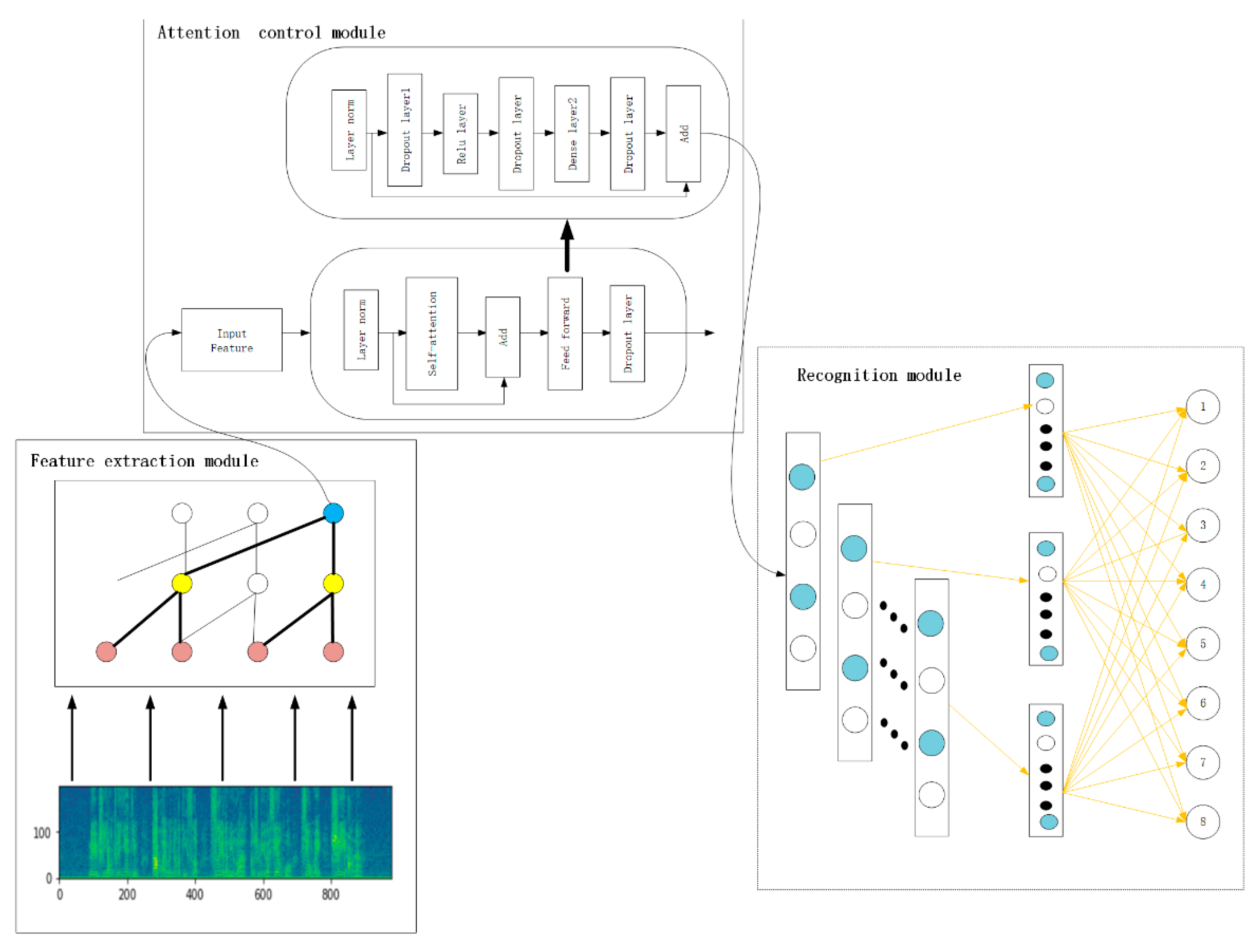
The model can be divided into three parts: the feature extraction module, attention mechanism control module and the recognizer model. The audio is converted into an image after the feature extraction module, and the image is processed by the CDCN so as to avoid information loss; then, it is transferred to the attention module to continuously pay attention to the contextual information, and finally it is transmitted to the classifier module to classify the audio, as shown in Figure 1.

The causal convolutional marker for initialization is a way to provide the initial transcription of training audio in order to start iterative training. Although these recognizers do indicate the use of transcribed audio, they can be considered a legacy resource. If the acoustic field of the legacy system is similar to the audio at hand, it can be very useful. The mismatch of the sound range will reduce the effectiveness of this recognizer. However, this is a fairly simple model, as each class has only one Gaussian value, and these methods can improve performance on the basis of the current Transformer initialization.

The encoder for traditional speech tasks uses the RNN to capture the temporal characteristics of speech and output higher-level features from the original input spectral features. Additionally, the latest architecture of the AED is the self-attentive structure proposed by Transformer of Neural Machine Translation (NMT), which learns the dependence of temporal information through temporal attention to the input features themselves, thus replacing the traditional RNN network layer. The key idea behind it is to generate a weighted average calculated by hidden units, using the information provided by the topic recognition system to dynamically obtain, round by round, the weights between the different components, which will depend on certain values obtained by the system, such as distance metric, similarity to the topic, etc. The interactions between the input signals depend on the signals themselves and are not predetermined by their relative positions as in the case of convolution. This allows the attention mechanism to capture remote interactions without increasing the number of parameters. In this way, we also evaluate the automatic clustering strategies, which are applied to the documents in the training dataset. The purpose is to create automatic topic clusters to verify whether these clusters can improve topic-based LMs compared with manually assigned topic tags of training datasets.

3.1. Feature Extraction

In speech feature extraction, this paper adopts the MFCC, which is the most common and effective algorithm for extracting sound features based on the principle of Cepstrum, which is more suitable for human hearing. In the calculation of the MFCC, the first step is to pre-aggravate the high frequency part of the speech signal to smooth the signal of the whole channel from low to high frequency, and at the same time, to eliminate the influence of the speaker in the process of occurrence. The continuous speech signal is divided into frames; each frame is multiplied by a Hamming window to improve the continuity between the left and right ends of the frame; after that, it needs to be converted into the energy distribution in the frequency domain, so that the transformation of speech signal in the time domain can more clearly express the characteristics of the signal, that is, the Fourier transformation process, so as to obtain the spectrum map distributed in different time windows on different time axes, as well as the analysis of gene frequency and formant.

The pre-processing work is performed on the audio in the dataset, because the audio length in the dataset is distributed around 4 s. In this experiment, the random offset/padding method is used to unify the audio lengths. Additionally, that is, a random window of 4 s is selected for audio longer than 4 s, and the excess is discarded, and a random back-and-forth zero complement is performed for audio shorter than 4 s. In this experiment, the sampling rate of audio is 16 k, so the length of the input is set to 16,000 × 4, which is the length of the audio after unification. To start the feature extraction of audio, this experiment uses Librosa’s audio manipulation toolkit, which provides a very powerful and easy way to manipulate audio. In the extraction of the previously mentioned features, Librosa is used to extract the MFCC, log-Mel and STFT features since the original waveform does not require much transformation and can be obtained directly. In terms of parameter settings, the MFCC is set to a MFCC of 40, frame shift of 320, and sampling rate of 16 k. The Mel filter of the Mel spectrum is set to 128. After extracting several features needed for the experiment, the extracted features are saved as feature files. The subsequent project is the training network part. For model building and training, this thesis uses the TensorFlow framework. There are three main reasons for using TensorFlow: the easy-to-use API, Python support, and dynamic computational graphs. Given the pre-trained Transformer network structure, we only select the most probable sound events to extract embedded features. We think $n=\left(n_1,n_2,n_3,\dots ,n_M\right)$ is a digital vector, where $M$ is the number of sound events defined in the UrbanSound8K dataset, and $n_i$ is the total number of times that the $i$-th sound event is detected in each program and used to mark the clip. The average embedding feature is calculated as $\overline{n_{\mathrm{i}}}=\frac{n_{\mathrm{i}}}{{{\displaystyle \sum }}_{\mathrm{i}=1}^{\mathrm{M}}{n}_{\mathrm{i}}}$. Given the embedding average, the baseline system divides them into 10 types.

In order to make our model more robust on small datasets and remove the noise contained in the original dataset, we reduce the dimensionality of the features. We use supervised and unsupervised forms such as Principal Component Analysis (PCA) and LDA to reduce the dimensionality of the data. It is found that the Stochastic Neighbor Embedding (SNE) algorithm has an obvious division effect on the dimensionality reduction in high-dimensional data. The high-dimensional data are represented by $X$, $Xi$ is the $i$-th sample, and $Y$ is the low-dimensional data. The distribution probability matrix $P$ in the high-dimensional is defined as:

$$P_{j|i}=\frac{exp(-\parallel x_i-x_j\parallel {}^2/2{\sigma }_i^2)}{{{\displaystyle \sum }}_{k\ne i}exp(-\parallel x_i-x_k\parallel {}^2/2{\sigma }_i^2)}$$

(1)

where P_j|i is the probability that the i-th sample is distributed around sample J. Sigma is determined according to the maximum entropy principle, $\mathrm{entropy}=\mathrm{H}\left(P_i\right)=-{{\displaystyle \sum }}_j{P}_{j|i}{log}_2{P}_{j|i}$. The Sigma centered on each sample point needs to make the entropy of the final distribution smaller, usually with $log\left(k\right)$ as the upper limit, where $k$ is the number of neighborhoods points you decide. Finally, the loss function is minimized by the gradient descent algorithm, and the convergence result is finally obtained. On the other hand, the low-dimensional distribution probability matrix is calculated as follows:

$$q_{j|i}=\frac{exp(-\parallel y_i-y_j\parallel {}^2)}{{{\displaystyle \sum }}_{k\ne i}exp(-\parallel y_i-y_k\parallel {}^2)}$$

(2)

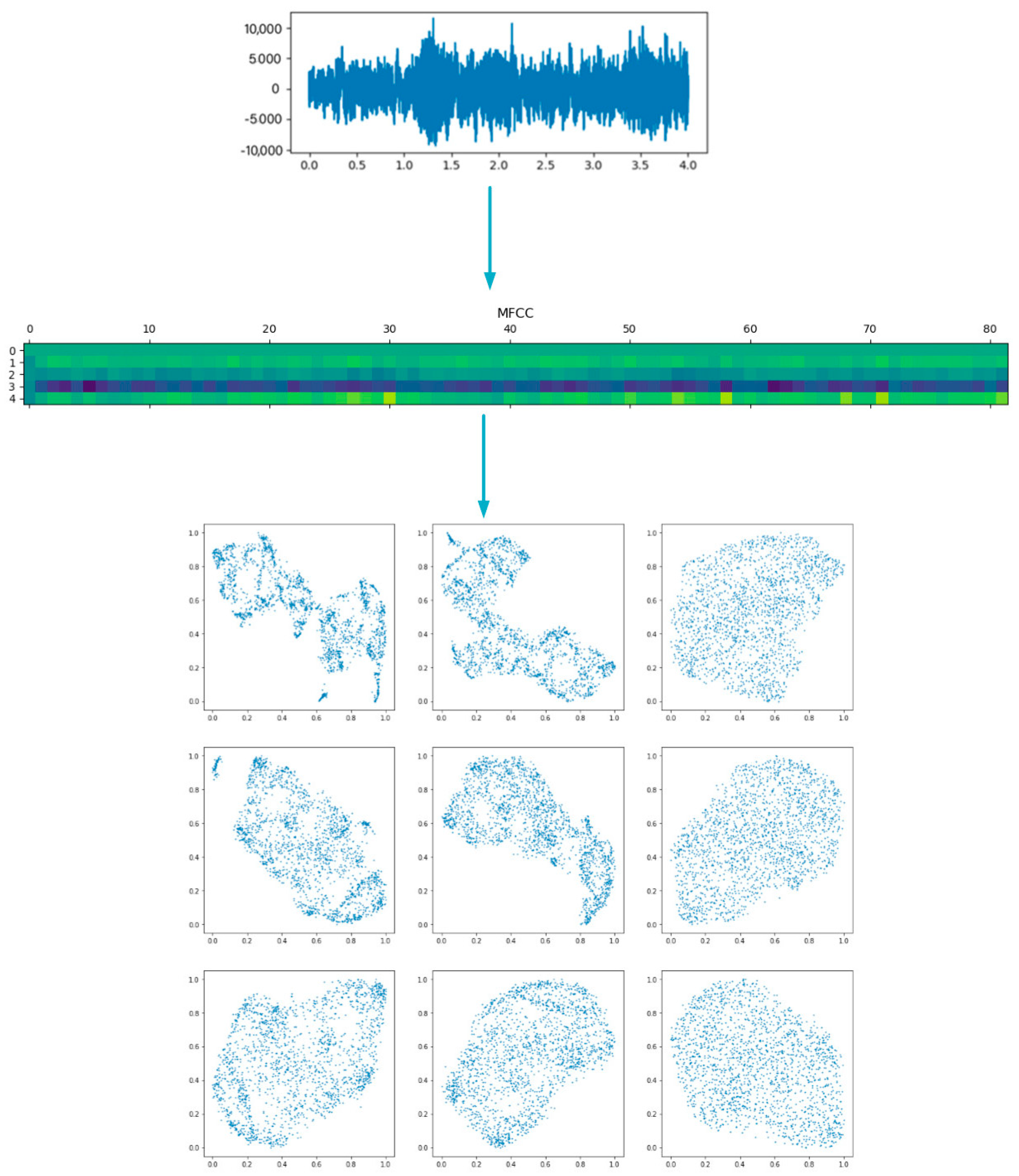
Select the audio feature extraction method such as (MFCCs or WaveNet) to extract hidden variables combined with different dimensionality reduction methods (uniform manifold approximation and projection (UMAP), t-SNE or PCA) to map UrbanSound8K data from multi-dimensional data to low-dimensional space, and the similarity with data points based on multiple features is used to try to distinguish the observation data group, so as to find the patterns of the data, as shown in Figure 2.

We can see from Figure 3 that there are some clusters of sounds. For two feature sets, sometimes, the local structure does not have similar sounds. The global structure can often show the sound trend. That is to say, in the upper part of the picture, most of the sounds are milder sounds of air conditioning and street music, the middle part are children playing and dogs barking, and the rest are sharp sounds such as gunshots and police sirens. We use WaveNet as the result of feature extraction to prove that these features are very robust when combined with dimensionality reduction technology. When compared with the graph obtained by the MFCC feature, there is no obvious degradation in the clustering. In other cases, compared with the MFCC with the same parameter settings, using the WaveNet vector actually improves the final graph.

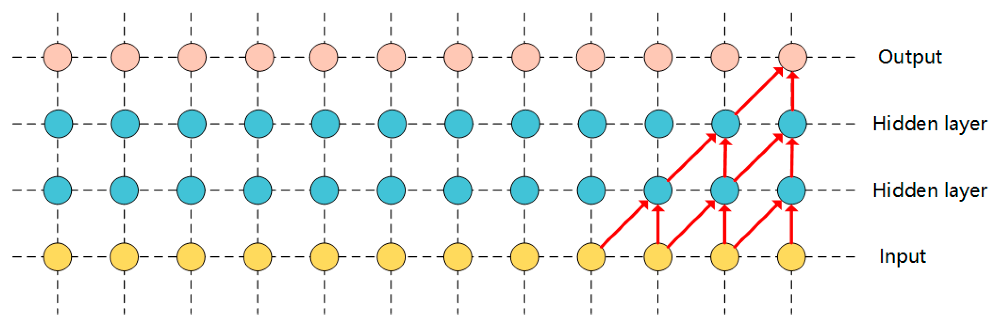
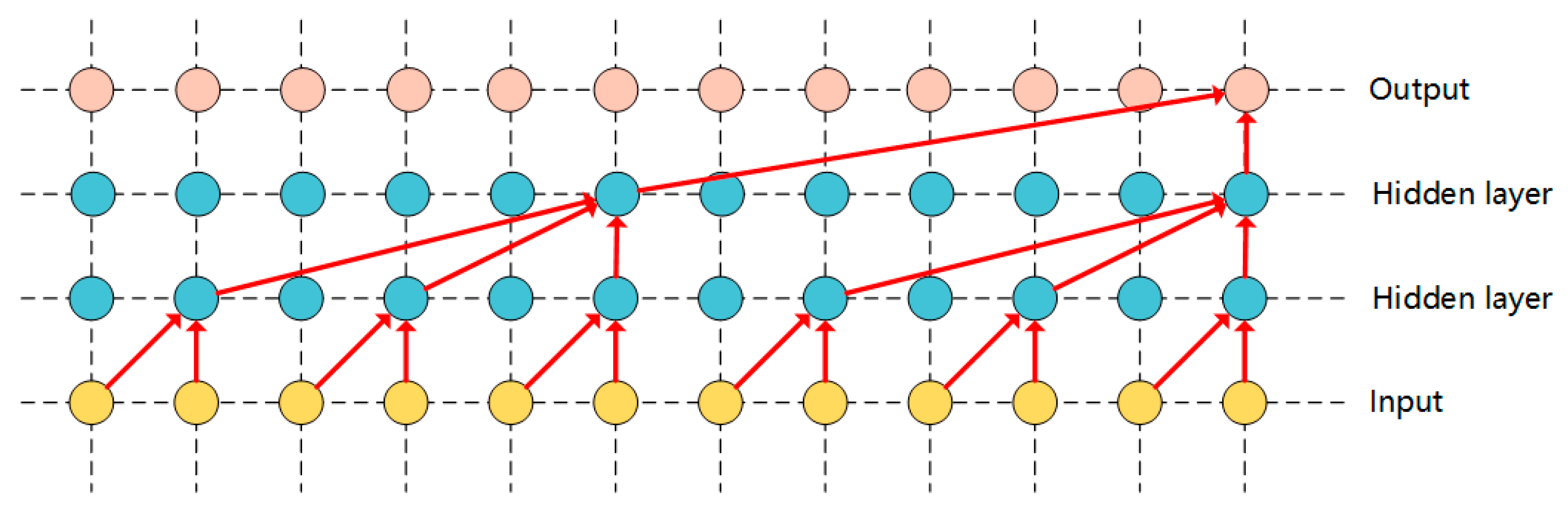
3.2. Hole Causal Convolution

An important part of speech recognition is causal convolution, which makes the model output consistent with the order of the data. The causal convolution model only uses the element before the element at time $t$, that is, time 0~t − 1 to predict the probability distribution of the current audio sample. It is a complete probabilistic autoregressive model. The combined probability of audio waveforms can be decomposed into a conditional probability distribution. The product of is as follows:

$$p\left(x\right)={\displaystyle \prod }_{t=1}^{T}p(x_t|x_1,\mathrm{\dots },x_{t-1})p\left(x\right)={\displaystyle \prod }_{t=1}^{T}p(x_t|x_1,\mathrm{\dots },x_{t-1})$$

(3)

Predict the value of the next point through the previous signal sequence, as shown in Figure 3. If this method is simply adopted, the final result will be that the receptive field is very small, and only a small amount of data can be used to generate the elements at time t. Therefore, in order to improve the perceptual range of the receptive field, the model proposes a stacked multi-layer convolution with holes to increase the receptive field of the network, so that the network can use more previous element values to generate the next element. Convolution with holes is a method for a convolution kernel to convolve data larger than itself. Compared with conventional convolution, perforated convolution can perform coarse-grained convolution operations. The structure diagram of the causal convolution model with holes is shown in Figure 4 and Figure 5:

3.3. Transformer

Transformer was first introduced by Vanswani et al. in machine translation, and then it was widely used in many tasks in the fields of Natural Language Processing (NLP), Computer Version (CV), and time-series (TS). Transformer is a network based on encoder–decoder. Its input is a sequence, and its output is also a sequence. In the encoder, the sequence is converted into a fixed-length vector, and then the vector is converted into the sequence we want through the decoder and output. For the encoder, self-attention can help the current node not only pay attention to the current word, so as to obtain the semantics of the context, which is more parallel than RNNs, but can also show superiority in large-scale training scenarios.

The advantage of realizing the complete End-To-End model by Transformer is that the self-attention mechanism is used to understand the current words with context, and the semantic feature extraction ability is stronger. It can filter the position of a single word or word in the whole statement, and obtain more accurate results. That is, the longer the sequence of sentences, the more abundant audio information it contains, the more accurate the recognition. Zhang et al. [23] used multiple feedforward self-attention layers to replace the RNN in the attention-based codec (AED) structure, so that the iteration speed of Transformer was faster in the training process and the generalization ability of Transformer in speech was changed.

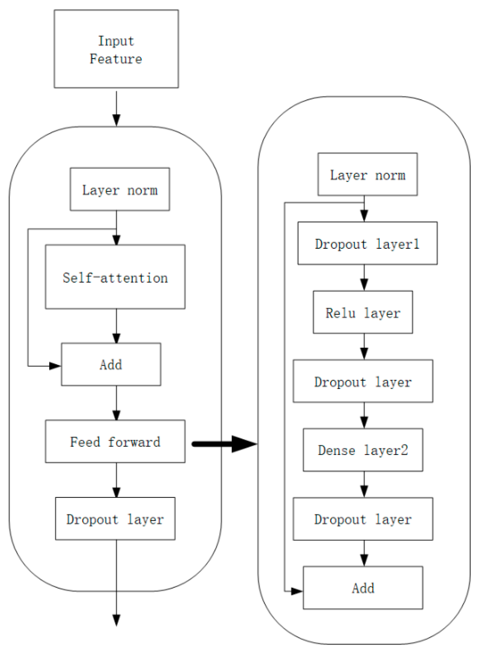
In the traditional hybrid ASR system, the acoustic model (AM), language model (LM) and pronunciation model (PM) are optimized independently to correspond with nonlinear sequences. The End-To-End approach adopted in this paper aims to simplify the ASR system by learning these models together in a single neural network. The AED model used in this article is composed of an encoder, a decoder, and an attention mechanism. The relevant features extracted from the encoder are output for the decoder to determine the token that needs to be output. The encoder usually uses the RNN model, and in order to improve the time series problem, this paper adopts the Causal Hole Convolution model, the decoder uses the Transformer, and generates the output token according to the context token and the encoder output order generation conditions. Our attention mechanism uses layer norm, which normalizes the hidden layer state dimensions to obtain an embedding that conforms to 0 means and variance is 1 Gaussian distribution. The formula is as shown in (4):

$$y=\frac{x-E\left|x\right|}{\sqrt{Var\left|X\right|+\in }}$$

(4)

Hierarchical normalization can greatly reduce the covariance deviation by modifying the mean and variance between the activation values in each layer. The feedforward module used in the architecture diagram is a simple fully connected feedforward network, which is marked by two fully connected and ReLU activation functions. The calculation formula is as follows:

$$FFN\left(x\right)=max(0,x{W}_1+b_1)W_2+b_2$$

(5)

Then, the input key value and feedforward are calculated and then the residual connection is added to form the final output of the multi-layer attention layer. Suppose the feedforward sublayer input is $x$, where $Sublayer\left(x\right)$ represents the function implemented by the sublayer itself, then the output is:

$$LayerNorm\left(x+SubLayer\left(x\right)\right)$$

(6)

After the output of the multi-layer feedforward header layer, the trainable parameter α is added to enable it to adapt to the data size output by the encoder and decoder, ${\mathrm{X}}_{\mathrm{i}}=\mathrm{prenet}({\mathrm{phoneme}}_{\mathrm{i}}+\mathsf{\alpha }\mathrm{PE}\left(\mathrm{i}\right)$, and a new variable is also introduced when calculating the output:

$$z_i={\displaystyle \sum }_{j=1}^n{\alpha }_{ij}\left(x_j{W}^v+a_{ij}^v\right)$$

(7)

The correlation between the input information can be measured and a weighted sum can be performed. In the feature extraction work, we have obtained a 128 × 4 t spectrogram, and then we split the spectrogram into N sequences of 16 × 16 slices, allowing the model to capture the spatial structure of the 2D audio spectrogram. In the attention control module, we use the original Transformer architecture; each module of encoder has two sub layers: the first is multi head self-attention layer, and the second is simple position by position full connection feedforward network. Then, dropout is applied to randomly inactivate the output of each sub layer. This process will be completed before adding sub layer input and performing normalization. See Figure 6 for more details.

In addition to the methods and rationale for using time-domain attention, this paper uses a CNN as the baseline system in the design of channel attention, passing the feature maps through the CNN and LSTM, respectively, and performing cosine similarity calculations on the results to obtain each channel weight by normalization. This design combines the ability of the CNN to process local information with the ability of the LSTM to perceive contextual information. Based on this theory and idea, the channel attention method is proposed and compared with the Transformer model to determine the classification ability of both.

4. Experimental Results

4.1. Experimental Environmental and Data

The deep neural network model is built on the Keras deep learning framework with TensorFlow as the backend, and the Python programming language is used to complete the entire experiment. The hardware and software environments of the experiment are shown in

Table 1. Experimental software and hardware environments.

Hardware and Software	Hardware and Hardware Configuration
CPU model	E5 series (8 cores)
GPU model	GTX 3060
RAM	16 G
Graphics card	NVIDIA 1070
Operating system	Ubuntu 16.04
Python	Python 3.7
Deep learning framework	Keras = 2.2.4 and TensorFlow = 1.15

.

This paper conducts two sets of topic recognition experiments in two different corpora.

The first set uses the UrbanSound8K dataset, which is a widely used public dataset for automatic urban environmental sound classification studies, and contains a total of 8732 labeled sound segments in 10 categories: air conditioning, car sirens, children playing, dogs barking, boreholes, engine idling, gunshots, handheld drills, sirens, and street music. The second uses the AudioSet corpus, which is taken from YouTube clip videos and consists of an extended ontology of 632 audio event classes covering a wide range of human and animal sounds, instruments and genres, and common everyday environmental sounds. They are often considered as a supervised learning problem in much sound event detection based on strongly labeled training data. However, generating a large number of strong labeled training data requires a lot of manpower, material resources, and is even mixed with a lot of human subjective judgment, which is not as effective as the weak labeled method in real life. Based on the weak marking method, this paper intercepts various types of audio of AudioSet as the data source.

In this experiment, a 10-fold cross-validation method is used to divide the screened audio dataset into 10 sets of samples, with one set as the test set and the remaining nine sets as the training set, ensuring that each set of audio signals traverses the test set once, and finally taking the average of the 10 test results.

In this experiment, Precision, Recall and F1-Score values are taken to evaluate the model comprehensively, as shown in Equations (8)–(10).

$$Precision=\frac{TP}{\left(TP+FP\right)}$$

(8)

$$Recall=\frac{TP}{\left(TP+FN\right)}$$

(9)

$$F1-Score=2\times \frac{Precision\times Recall}{Precision+Recall}=\frac{2TP}{2TP+FP+FN}$$

(10)

Among them, $TP$ denotes the number of predicted and actual correctly classified labels, $FP$ denotes the combing of misclassified labels in the predicted labels, and $FN$ denotes the number of misclassified labels in the actual labels.

4.2. Experimental Setup

In the data pre-training, the accuracy of audio feature extraction is low, and the over-fitting situation is obvious. Therefore, this experiment has retrained to improve the model and parameters. For regularization, use dropout for each residual cell, P_drop = 0.2, use Adam optimizer, use categorical_crossentropy loss to improve the effect of feature extraction. According to the number of samples and pre-training results, the parameters of the finally set model are shown in

Table 2. Model parameters.

Layer Number	Layer Name	Comments
Layer 1	front/conv1d	Fully connected layer
Layer 2	front/BN	Batch normalization
Layer 3	block_0_1/conv_filter	dilation = 1 convolution
Layer 4	block_0_1/BN	Batch normalization
Layer 5	block_0_1/conv_gate	dilation = 1 convolution
Layer 6	block_0_1/BN	Batch normalization
Layer 7	block_0_1/multi_matrix	element—wise chengfa
Layer 8	block_0_1/conv_out	Fully connected layer
Layer 9	block_0_1/BN	Batch normalization
Layer 10	block_0_1/residual connect	Residual connection

:

4.3. Evaluation

For evaluation, we measured the performance of our proposed model on training data and test data. In order to verify the performance of the proposed model, we analyzed the number of parameters, confusion matrix and measurement parameters such as accuracy, recall, and F-score.

Use the above TCDCN model and CNN-LSTM, CNN-CTC, and XGBoost models to train the noise-free training set. The test set also uses noise-free audio. The network configuration of each comparison model is introduced below:

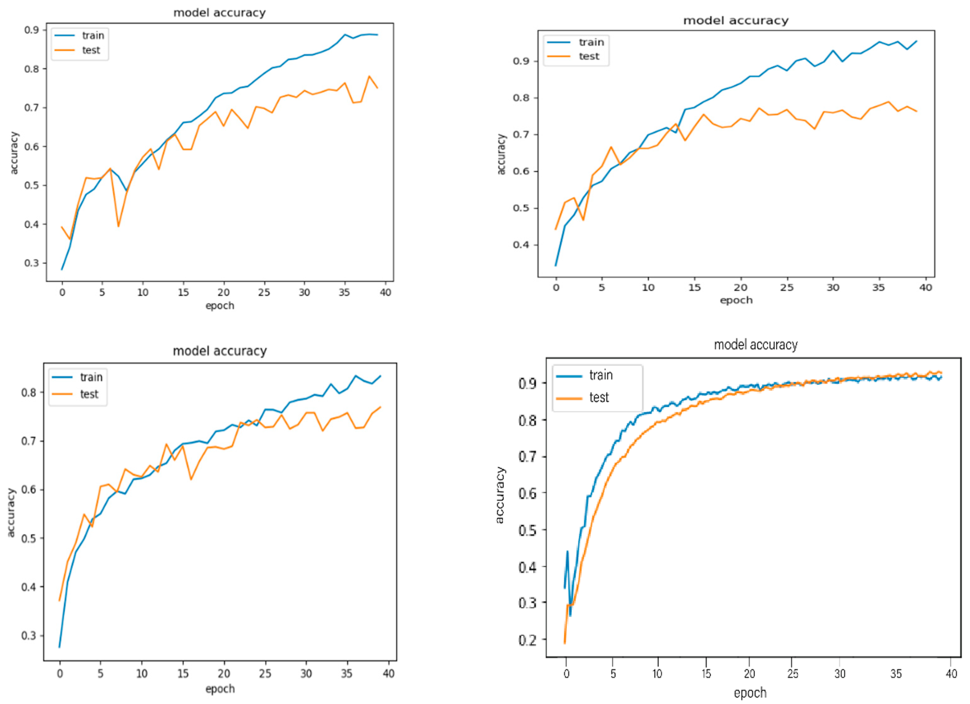
For the audio event classification task, we used the previously proposed model architecture and optimizer, trained for 40 epochs. Figure 7 shows the accuracy variation of the four networks on the validation set, while saving the weights of the networks for the period with the largest F1 values in the validation set.

Table 3. Result of Accuracy VALUES on the test set.

Model	Architecture	F1 (%)
CNN-CTC	3 conv + 8 batch norm + 3 max-pooling layers	71.4
CNN-LSTM	4conv + 2Maxpooling + LSTM	73.0
TCDCN XGBOST	transformer encoder and decoder + dilation 3 conv + 2Maxpooling + XGBoost	89.8 78.4

shows the overall detection results.

Figure 8 shows the prediction results for each classification model for the UrbanSound8K dataset. One of the larger errors is the partial similarity between the sounds of children playing and the street music scene, leading to a reduction in classification accuracy. Overall, compared with the traditional model structure and the speech model based on attention mechanism, the structure of the TCDCN model is far more complex than other models. Through the multi-layer hole convolution, the perception field can be expanded, and the fitting of context relevance is strong, so the final topic recognition rate is raised. To further validate the classification performance of the TCDCN hybrid model, we chose the publicly available audio scene dataset AudioSet for testing, and the test results are shown in

Table 4. Performance of the proposed systems on the validation (Val.).

Systems	Network Structure	Input Feature	VAL.AT
			Accuracy	F1	P	R
CNN	3conv + 2Maxpooling	Mel-Spectrogram	71%	0.71	63.4%	63.5%
XGBoost	——	log-mel	83%	0.82	83.2%	82.4%
CNN-XGBoost	3conv + 2Maxpooling+XGBoost	log-mel	89%	0.88	89.2%	87.2%
CNN-LSTM	4conv + 2Maxpooling + LSTM	Mel-Spectrogram	84	0.81	83.1%	82.7%
TCDCN	8conv + 4Maxpooling	Mel-Spectrogram	91	0.90	89.5%	88.7%
CRNN(Dropout)	3conv + 2Maxpooling + LSTM	Mel-Spectrogram	73%	0.72	65.5%	65.7%

. From Table 4, we can conclude that the classification performance of the hybrid model is significantly better than that of the individual model.

5. Conclusions and Future Outlook

This paper is a useful exploration of the Transformer model in speech recognition. In the transition from the DNN–HMM era of speech recognition to the End-To-End era, the multilayer hole causal convolution structure based on the TCDCN model of End-To-End technology provides a good attempt of the development of acoustic model and speech recognition. The biggest advantage of Transformer over the RNN lies in its speed advantage. Compared with the CNN, it can directly obtain global information. In the process of speech recognition, the increase in the receptive field is particularly important to the long-term dependence on the modeled speech signal. The model combines causal convolution and hole convolution, so that the receptive field increases exponentially with the training depth of the model, which also makes it stand out in many models. This paper uses the MFCC feature extraction method to extract the voice features, and then processes it through the deep convolutional neural network; to address the problem of the low correct classification rate of audio scenes, this paper adopts a hybrid model of the TCDCN, making full use of the feature that the CDCN can extract more information and Transformer’s strong focus on time-related information, so that the classification of the hybrid model achieves an average accuracy of 89% on the UrbanSound8K dataset. The experimental results show that the TCDCN is better than the traditional neural network model, thus verifying that the combination of these two models can be well suited for audio scene classification tasks.

As an application of the field of artificial intelligence, speech recognition has been widely used in real scenes, but the recognition scene still poses a challenge to the recognition technology. As a complete End-To-End model of the new paradigm of speech recognition, it is a change in the field of speech recognition. Google, Baidu and other teams have also put forward their own End-To-End recognition models. Due to the limitations of time and the author’s level, this article has not achieved enough comparisons of multiple corpus and multiple models in experimental comparison. In the future, we are also eager to make effective attempts on the End-To-End deep learning model based on the attention mechanism.

References

- Levinson, S.E.; Rabiner, L.R.; Sondhi, M.M. An Introduction to the Application of the Theory of Probabilistic Functions of a Markov Process to Automatic Speech Recognition. Bell Syst. Tech. J. 1983, 62, 1035–1074. [Google Scholar] [CrossRef]
- Lee, K.F.; Hon, H.W. Speaker-independent phone recognition using hidden Markov models. IEEE Trans. Acoust. Speech Signal Process. 1989, 37, 1641–1648. [Google Scholar] [CrossRef] [Green Version]
- Deng, L.; Aksmanovic, M. Speaker-Independent phonetic classification using hidden Markovmodels with mixtures of trend functions. IEEE Trans. Speech Audio Process. 1997, 5, 319–324. [Google Scholar] [CrossRef]
- Mohamed, A.; Dahl, G.; Hinton, G. Deep Belief Networks for phone recognition. Scholarpedia 2009, 4, 1–9. [Google Scholar]
- Povey, D.; Ghoshal, A.; Boulianne, G.; Burget, L.; Vesel, K. The Kaldi speech recognition toolkit. In Proceedings of the IEEE 2011 Workshop on Automatic Speech Recognition and Understanding, Waikoloa, HI, USA, 11–15 December 2011. [Google Scholar]
- Sak, H.I.; Senior, A.; Rao, K.; Beaufays, F.O. Fast and Accurate Recurrent Neural Network Acoustic Models for Speech Recognition. Comput. Sci. 2015. [Google Scholar]
- Bellegarda, J.R. Statistical language model adaptation: Review and perspectives. Speech Commun. 2004, 42, 93–108. [Google Scholar] [CrossRef]
- Echeverry-Correa, J.D.; Ferreiros-López, J.; Coucheiro-Limeres, A.; Córdoba, R.; Montero, J.M. Topic identification techniques applied to dynamic language model adaptation for automatic speech recognition. Expert Syst. Appl. 2015, 42, 101–112. [Google Scholar] [CrossRef]
- Siu, M.H.; Gish, H.; Chan, A.; Belfield, W.; Lowe, S. Unsupervised training of an HMM-Based self-organizing unit recognizer with applications to topic classification and keyword discovery. Comput. Speech Lang. 2014, 28, 210–223. [Google Scholar] [CrossRef]
- Takahashi, S. Topic-Specific Language Model Based on Graph Spectral Approach for Speech Recognition. In Trends in Intelligent Systems and Computer Engineering; Castillo, O., Xu, L., Ao, S.-I., Eds.; Springer: Boston, MA, USA, 2008; pp. 497–514. [Google Scholar]
- Bengio, Y.; Schwenk, H.; Senécal, J.-S.; Morin, F.; Gauvain, J.-L. Neural Probabilistic Language Models. In Innovations in Machine Learning: Theory and Applications; Holmes, D.E., Jain, L.C., Eds.; Springer: Heidelberg/Berlin, Germany, 2006; pp. 137–186. [Google Scholar]
- Tanaka, T.; Masumura, R.; Oba, T. Neural candidate-aware language models for speech recognition. Comput. Speech Lang. 2020, 66. [Google Scholar] [CrossRef]
- Rathor, S.; Agrawal, S. A robust model for domain recognition of acoustic communication using Bidirectional LSTM and deep neural network. Neural Comput. Appl. 2021, 1–10. [Google Scholar] [CrossRef]
- Lin, C.-H.; Tu, M.-C.; Chin, Y.-H.; Liao, W.-J.; Hsu, C.-S.; Lin, S.-H.; Wang, J.-C.; Wang, J.-F. SVM-Based Sound Classification Based on MPEG-7 Audio LLDs and Related Enhanced Features. In Proceedings of the International Conference on Hybrid Information Technology, Daejeon, Korea, 23–25 August 2012; pp. 536–543. [Google Scholar]
- Jones, G.J.F. About Sound and Vision: CLEF Beyond Text Retrieval Tasks. In Information Retrieval Evaluation in a Changing World: Lessons Learned from 20 Years of CLEF; Ferro, N., Peters, C., Eds.; Springer International Publishing: Cham, Switzerland, 2019; pp. 307–329. [Google Scholar]
- Huang, T.C.; Hsieh, C.H.; Wang, H.C. Automatic meeting summarization and topic detection system. Data Technol. Appl. 2018, 52, 351–365. [Google Scholar] [CrossRef]
- Łopatka, K.; Kotus, J.; Czyżewski, A. Evaluation of Sound Event Detection, Classification and Localization in the Presence of Background Noise for Acoustic Surveillance of Hazardous Situations. In Proceedings of the Multimedia Communications, Services and Security, Krakow, Poland, 11–12 June 2014; pp. 96–110. [Google Scholar]
- Vozáriková, E.; Juhár, J.; Čižmár, A. Acoustic Events Detection Using MFCC and MPEG-7 Descriptors. In Proceedings of the International Conference on Multimedia Communications, Services and Security, Krakow, Poland, 2–3 June 2011; pp. 191–197. [Google Scholar]
- Bost, X.; Senay, G.; El-Bèze, M.; Mori, R.D. Multiple topic identification in human/human conversations. Comput. Speech Lang. 2015, 34, 18–42. [Google Scholar] [CrossRef] [Green Version]
- Zinemanas, P.; Cancela, P.; Rocamora, M. End-to-end Convolutional Neural Networks for Sound Event Detection in Urban Environments. In Proceedings of the 24th IEEE FRUCT, Moscow, Russia, 8–12 April 2019. [Google Scholar]
- Kong, Q.; Xu, Y.; Wang, W.; Plumbley, M. Sound Event Detection of Weakly Labelled Data with CNN-Transformer and Automatic Threshold Optimization. IEEE/ACM Trans. Audio Speech Lang. Process. 2020, 28, 2450–2460. [Google Scholar] [CrossRef]
- Kong, Q.; Yong, X.; Wang, W.; Plumbley, M. Audio Set Classification with Attention Model: A Probabilistic Perspective. In Proceedings of the International Conference on Acoustics, Speech, and Signal Processing, ICASSP 2018, Calgary, AB, Canada, 15–20 April 2018; pp. 316–320. [Google Scholar]
- Zhang, Q.; Lu, H.; Sak, H.; Tripathi, A.; Mcdermott, E.; Koo, S.; Kumar, S. Transformer Transducer: A Streamable Speech Recognition Model with Transformer Encoders and RNN-T Loss. In Proceedings of the ICASSP 2020–2020 IEEE International Conference on Acoustics, Speech and Signal Processing (ICASSP), Barcelona, Spain, 4–8 May 2020. [Google Scholar]