Leader-Follower Formation Control of Wheeled Mobile Robots without Attitude Measurements

Abstract

The problem of leader-follower formation of a platoon of differential-drive wheeled mobile robots without using attitude measurements is addressed in this paper. Contrary to the position-distance approaches existing in the literature, the formation and collision avoidance is achieved by introducing a state-dependent delay in the desired trajectory. The delay is obtained as the output of a dynamical system and its magnitude will decrease/increase depending on the distance between the robots. To guarantee trajectory tracking and to overcome the lack of orientation measurements, an output feedback control and attitude observer are proposed based on the kinematic model of the robots. The attitude observer is designed directly on the special orthogonal group $SO(2)$ and it can be used in open-loop schemes. The proposed control-observer scheme ensures asymptotic convergence of the tracking and observer errors. Finally, experimental results are presented to show the performance of the proposed approach.

1. Introduction

In recent years, autonomous mobile vehicles have attracted interest from the scientific community, mainly due to the wide range of applications in which they can be implemented; ranging from searching, surveillance and exploration applications to cargo transportation and cooperative manipulation [1,2]. Cooperative formation control focuses more on the efficiency and fault tolerance that a single mobile robot could not provide [3]. A particular problem of multi-robot coordination that has received much attention in the last decades is formation control. The objective of formation control of multiple mobile robots is to achieve a desired formation pattern while guaranteeing that the multiple robots as a group accomplish a given task cooperatively [4].

The formation control approach has been implemented in different types of vehicles, this in order to perform the tasks, with greater ease and robustness. For example, in [5] this approach was used for underwater vehicles, where the follower tracks a reference trajectory based on the leader position and predetermined formation without the need for leader’s velocity and dynamics. This is desirable in marine robotics due to weak underwater communication and low bandwidth. In order to tackle the harsh conditions of underwater environment, in [6] the authors drive unmanned underwater vehicle using a deterministic artificial intelligence approach. This technique is based on self-awareness of the robot and relies on the dynamic of the vehicle and linear regression instead of stochastic or traditional control theory methods. Another application of this technique is presented in [7], where the authors address formation control for a team of quadrotor UAVs in which the robots follow a specified group trajectory while safely changing the shape of the formation according to the specifications of the task. On the other hand, in [8] the formation control of a group of unicycle-type wheeled mobile robots at the dynamics level with a little amount of inter-robot communication is investigated. Another interesting approach arises from bio-inspired control techniques. The robotic swarm control is a new paradigm of multi-robot control system aiming to achieve task in collective way using low level interactions between the members of the swarm. For instance, in [9] the authors proposed to employ a variation of the particle swarm optimization (PSO) algorithm to achieve formation in a swarm of agents while tracking a dynamic target. This techniques is inspired on the pheromone based communication of the ant colonies.

Several formation control approaches have been proposed in the literature, and they are mainly divided in three categories: behavior-based methods, leader–follower and virtual structure methods [10,11]. The behavior-based approach is inspired by the emerging behaviors in nature such as flock of birds, random walks of ants and school of fish [12]. In this case, a group behavior (or mission) comprises some low-level actions (or sub-tasks) and is constructed to achieve the global objective, where the individual robot needs to perform low-level actions to accomplish the group behavior [13]. In the leader-follower formation [14,15], one robot is chosen as the leader which decides the whole formation group’s moving trajectory, the other ones are the followers which are tasked to follow the leader, and the desired relative separations and bearings are expected to be maintained [16]. This strategy is easily implemented by using two controllers only and is suitable to describe the formation of robots, but it is hard to take into account the functioning capabilities of different robots, i.e., ability gap of a robot [17]. Finally, in the virtual structure formation, robots behave like particles embedded in a rigid virtual structure [18].

Some very interesting works where the leader-follower formation is used are, for example [19], in which the formation problem is converted to a trajectory tracking problem, where each follower robot tracks its corresponding generated reference trajectory such that the whole group forms and maintains the desired shape. In this work, some experiments were successfully conducted and reported using a group of four TURTLEBOTs. In [20], the authors tackle the leader-follower formation control problem of non-holonomic mobile robots. In this case, the trajectory tracking control for a single non-holonomic mobile robot is extended to the formation control for two non-holonomic robots in which one is the leader and the second is the follower. The controllers proposed by the authors are based on the PI control technique. Simulation results are presented to demonstrate the good performance of the proposed controller.

In this work, we addressed the leader-follower formation control problem for a group of nonholonomic wheeled mobile robots (WMRs). We do not follow the common distance-based approaches where the follower tracks the trajectory generated by the leader with an offset to avoid a collisions. In our approach, the followers track the delayed desired trajectory of the leader. The time delay is not arbitrary, on the contrary, it is obtained as the output of a dynamical system whose inputs are the position of the robots. The aforementioned dynamical system is designed in such way that, when the distance between the robots increases, the magnitude of the delay decreases and vice versa. The proposed methodology allows to achieve a convoy formation or platooning without collisions. Another advantage of the proposed approach is that the followers do not deviate from the leader’s path during cornering [21] like the distance-based approaches. Moreover, the distance between robots can be modified by simple tuning the parameters of the delay’s dynamical system. To track the desired trajectory, a novel control is proposed that exploits the cascade structure of the robot’s kinematic model.

On the other hand, one of the most common problems during the implementation of controllers is the lack of state measurements such as velocity, acceleration, orientation, to name a few. This absence of information could be treated by using different sensors to mediate it. However, this would make the system more complex and above all more expensive. Another factor, for example, is that accurate velocity measurements can be difficult, and actually, may be contaminated by the noises in real environments, which can deteriorate the control performance [22].

One of the alternatives to solve the problem of lack of information, is the design of state observers to estimate the measures that the controller needs. There are many works that use observers to estimate information of a system. In [23], the Cartesian position and the kinematic model is employed to design nonlinear observers to estimate the orientation angle and the linear velocity of a mobile robot. On the other hand, in [24] a state-feedback controller for the non-linear error dynamics of the robot is combined with an observer that estimates the orientation error based on available trajectory information and measurement of the position coordinates. Furthermore, in [25] kinematic and dynamic models of the WMR are described, and an output feedback controller is proposed using adaptive sliding mode controller and a high gain observer is designed for velocity estimation to obtain WMR trajectory tracking.

In this paper, we assume that only the Cartesian position and its time derivative are available from measurements. To overcome the lack of attitude measurements a nonlinear observer is proposed based on the kinematic model of the robot. The orientation observer is designed directly on $SO(2)$ and can be used in either open and closed loop schemes. The stability analysis is carried out by means of Lyapunov theory.

The rest of the paper is organized as follows: In Section 2 the kinematic model of a unicycle mobile robot is presented. The design of the attitude observer and its stability analysis is presented in Section 3, and in Section 4, the control algorithm for Leader-follower formation is described. In Section 5 the stability analysis for the complete closed-loop system is presented. Experimental results with a group of three wheeled mobile robots are presented in Section 6. Finally, conclusions and future research directions are stated in Section 6.

2. Kinematic Model

Consider a group of differential-drive mobile robots as it is shown in the Figure 1. According to the figure, the Cartesian position and orientation of each robot are denoted by ${\mathit{x}}_i=\mathrm{col}(x_i,y_i)\in {\mathfrak{R}}^2$ and ${\theta }_i\in \mathfrak{R}$, respectively. The posture of each robot can be described by the unicycle kinematic model as follows

$${\stackrel{·}{\mathit{x}}}_{\mathrm{i}}={\mathsf{\Theta }}_i{\nu }_{\mathrm{i}},$$

(1a)

$${\stackrel{·}{\theta }}_i={\omega }_i,i=\ell ,{\mathrm{f}}_j,j=1,\dots ,n,$$

(1b)

where ${\mathsf{\Theta }}_i\triangleq \mathrm{col}(\cos ({\theta }_i),\sin ({\theta }_i))\in {\mathfrak{R}}^2$ represents the direction of the Cartesian velocity and n is the number of slave robots. Finally, ${\nu }_i$ and ${\omega }_i$ are the linear and angular velocities, respectively. The orientation angle and the Cartesian velocity satisfy the nonholonomic constraint

$${\stackrel{·}{y}}_{\mathrm{i}}\cos ({\theta }_{\mathrm{i}})-{\stackrel{·}{x}}_{\mathrm{i}}\sin ({\theta }_{\mathrm{i}})=0$$

(2)

or equivalently,

$$\tan ({\theta }_{\mathrm{i}})=\frac{{\stackrel{·}{y}}_{\mathrm{i}}}{{\stackrel{·}{x}}_{\mathrm{i}}}.$$

(3)

The nonholonomic constraint (3) implies that the velocity in the direction of wheel axis is zero, i.e., the robot cannot move in the lateral directions.

3. Attitude Observer

In order to develop the attitude observer, first notice that an equivalent representation of the kinematic model (1) is the following

$${\stackrel{·}{\mathit{x}}}_i={\nu }_i{\mathit{R}}_i{\mathit{e}}_1,{\mathit{e}}_1=\mathrm{col}(1,0)$$

(4a)

$$\stackrel{·}{\mathit{R}}={\omega }_i{\mathit{S}\mathit{R}}_i$$

(4b)

where ${\mathit{R}}_i=\left[\begin{array}{cc}{\mathsf{\Theta }}_i& \mathit{S}{\mathsf{\Theta }}_i\end{array}\right]\in \mathcal{S}\mathcal{O}(2)=\{\mathit{R}\in {\mathfrak{R}}^{2\times 2}|{\mathit{R}}^{\top }\mathit{R}=\mathit{I},\mathrm{de}(\mathit{R})=+1\}$ is the rotation matrix and $\mathit{S}\in {\mathfrak{R}}^{2\times 2}$ is a skew-symmetric matrix given by

$$\mathit{S}=\left[\begin{array}{cc}0& -1\\ 1& 0\end{array}\right].$$

(5)

For the case of $SO(2)$ the rotation matrix ${\mathit{R}}_i$ and skew-symmetric matrix $\mathit{S}$ commute, i.e., ${\mathit{S}\mathit{R}}_i={\mathit{R}}_i\mathit{S}$. On the other hand, from (1a) the rotation matrix ${\mathit{R}}_i$ can be reconstructed in an algebraic way as follows

$$\mathit{R}=\left[{\mathit{v}}_i{\mathit{S}\mathit{v}}_i\right],{\mathit{v}}_i\triangleq \frac{{\stackrel{·}{\mathit{x}}}_i}{\parallel {\stackrel{·}{\mathit{x}}}_i\parallel }$$

(6)

as long as $\parallel {\stackrel{·}{\mathit{x}}}_i(t)\parallel \nrightarrow 0$ for all $t\ge 0$. Based on the foregoing equation, the attitude observation error is defined as

$$\begin{array}{c}\hfill {\tilde{\mathit{R}}}_i={\widehat{\mathit{R}}}_i^{\top }{\mathit{R}}_i\end{array}$$

(7)

where ${\widehat{\mathit{R}}}_i=\left[\begin{array}{cc}{\widehat{\mathsf{\Theta }}}_i& \mathit{S}{\widehat{\mathsf{\Theta }}}_i\end{array}\right]\in \mathcal{S}\mathcal{O}(2)$ and ${\widehat{\mathsf{\Theta }}}_i$ are estimates of ${\mathit{R}}_i$ and ${\mathsf{\Theta }}_i$, respectively. With the previous definition the objective is to design an attitude observer such that ${\tilde{\mathit{R}}}_i(t)\to \mathit{I}$ as $t\to \infty$ where $\mathit{I}\in {\mathfrak{R}}^{2\times 2}$ is the identity matrix. Motivated by the work reported in [26] the following attitude observer is proposed

$$\begin{array}{cc}\hfill {\stackrel{·}{\widehat{\mathit{R}}}}_i& ={\widehat{\omega }}_i\mathit{S}{\widehat{\mathit{R}}}_i\hfill \end{array}$$

(8a)

$$\begin{array}{cc}\hfill {\widehat{\omega }}_i& ={\omega }_i+k_{\mathrm{a}i}{\mathit{v}}_i^{\top }\mathit{S}{\widehat{\mathsf{\Theta }}}_i\hfill \end{array}$$

(8b)

where $k_{\mathrm{a}i}\in \mathfrak{R}$ is a positive constant and ${\mathit{v}}_i\in {\mathfrak{R}}^2$ is given in (6). Notice that the proposed attitude observer can be used in open-loop schemes. Now we can establish the first result of the paper.

Theorem 1.

Assume that the angular velocity ${\omega }_i$ and the Cartesian velocity ${\stackrel{·}{\mathit{x}}}_i$ are available. Moreover, assume that the robot’s motion satisfies $\parallel {\stackrel{·}{\mathit{x}}}_i(t)\parallel \nrightarrow 0$ ∀ $t\ge 0$. Then, the attitude observer given in (8) guarantees that ${\tilde{\mathit{R}}}_i\to \mathit{I}$ as $t\to \infty$.

Proof. 

By taking into account (4b) and (8) the time derivative of the attitude observation error (7) is given by

$$\begin{array}{cc}\hfill {\stackrel{·}{\stackrel{~}{\mathit{R}}}}_i& ={\stackrel{·}{\widehat{\mathit{R}}}}_i^{\top }{\mathit{R}}_i+{\widehat{\mathit{R}}}_i^{\top }{\stackrel{·}{\mathit{R}}}_i\hfill \\ & =\left({\omega }_i-{\widehat{\omega }}_i\right){\widehat{\mathit{R}}}_i^{\top }{\mathit{S}\mathit{R}}_i\hfill \\ & =\left({\omega }_i-{\widehat{\omega }}_i\right){\tilde{\mathit{R}}}_i\mathit{S}.\hfill \end{array}$$

(9)

where ${\mathit{R}}_i\mathit{S}=\mathit{S}{\mathit{R}}_i$ has been used. Now consider the positive scalar function

$$\begin{array}{c}\hfill V_{\mathrm{R}i}=\frac{1}{2}\mathrm{tr}(\mathit{I}-{\tilde{\mathit{R}}}_i)\end{array}$$

(10)

whose time derivative along (9) is given by

$$\begin{array}{cc}\hfill {\stackrel{·}{V}}_{\mathrm{R}i}& =-\frac{1}{2}\left({\omega }_i-{\widehat{\omega }}_i\right)\mathrm{tr}({\tilde{\mathit{R}}}_i\mathit{S})\hfill \\ & =\frac{1}{2}{k}_{{\mathrm{a}}_i}\left({\mathit{v}}_i^{\top }\mathit{S}{\widehat{\mathsf{\Theta }}}_i\right)\mathrm{tr}({\tilde{\mathit{R}}}_i\mathit{S}).\hfill \end{array}$$

(11)

By taking into account (6), the elements of ${\tilde{\mathit{R}}}_i$ can be expressed as

$${\tilde{\mathit{R}}}_i=\left[\begin{array}{cc}{\mathit{v}}_i^{\top }{\widehat{\mathsf{\Theta }}}_i& -{\mathit{v}}_i^{\top }\mathit{S}{\widehat{\mathsf{\Theta }}}_i\\ {\mathit{v}}_i^{\top }\mathit{S}{\widehat{\mathsf{\Theta }}}_i& {\mathit{v}}_i^{\top }{\widehat{\mathsf{\Theta }}}_i\end{array}\right].$$

(12)

Therefore, the trace of the matrix ${\tilde{\mathit{R}}}_i\mathit{S}$ is given by

$$\mathrm{tr}({\tilde{\mathit{R}}}_i\mathit{S})=-2{\mathit{v}}_i^{\top }\mathit{S}{\widehat{\mathsf{\Theta }}}_i.$$

(13)

Substituting the previous result in (11) yields

$${\stackrel{·}{V}}_{\mathrm{R}i}=-k_{{\mathrm{a}}_i}{\left({\mathit{v}}_i^{\top }\mathit{S}{\widehat{\mathsf{\Theta }}}_i\right)}^2<0$$

(14)

Therefore $V_{\mathrm{R}i}$ converges asymptotically to zero, this in turn implies that ${\tilde{\mathit{R}}}_i\to \mathit{I}$ as $t\to \infty$. This completes the proof. □

4. Formation Control Algorithm

The kinematic model (1) is an underactuated nonlinear system. To overcome this problem, consider the auxiliary control input

$${\mathit{u}}_i={\nu }_i{\mathit{R}}_{\mathrm{d}}{\mathit{e}}_1={\nu }_i{\mathsf{\Theta }}_{\mathrm{d}i}$$

(15)

where ${\mathit{R}}_{\mathrm{d}i}=\left[\begin{array}{cc}{\mathsf{\Theta }}_{\mathrm{d}i}& \mathit{S}{\mathsf{\Theta }}_{\mathrm{d}i}\end{array}\right]\in SO(2)$ represents the desired orientation with ${\mathsf{\Theta }}_{\mathrm{d}i}=\mathrm{col}(\cos ({\theta }_{\mathrm{d}i}),\sin ({\theta }_{\mathrm{d}i}))$. Therefore, the kinematic model can be written as

$$\begin{array}{cc}\hfill {\stackrel{·}{\mathit{x}}}_i& ={\mathit{u}}_i+{\nu }_i({\mathsf{\Theta }}_i-{\mathsf{\Theta }}_{\mathrm{d}i})\hfill \end{array}$$

(16a)

$$\begin{array}{cc}\hfill {\stackrel{·}{\theta }}_i& ={\omega }_i.\hfill \end{array}$$

(16b)

In this case, the translational subsystem given by (16a) can be analyzed as a completely actuated system perturbed by the coupling term ${\nu }_i({\mathsf{\Theta }}_i-{\mathsf{\Theta }}_{\mathrm{d}i})$ which relates the translational subsystem with the attitude subsystem (16b). On the other hand, given the control input ${\mathit{u}}_i$ the desired vector ${\mathsf{\Theta }}_{\mathrm{d}i}$ and ${\nu }_i$ can be computed as

$${\mathsf{\Theta }}_{\mathrm{d}i}=\frac{{\mathit{u}}_{\mathrm{i}}}{\parallel {\mathit{u}}_i\parallel },{\nu }_i=\parallel {\mathit{u}}_i\parallel .$$

(17)

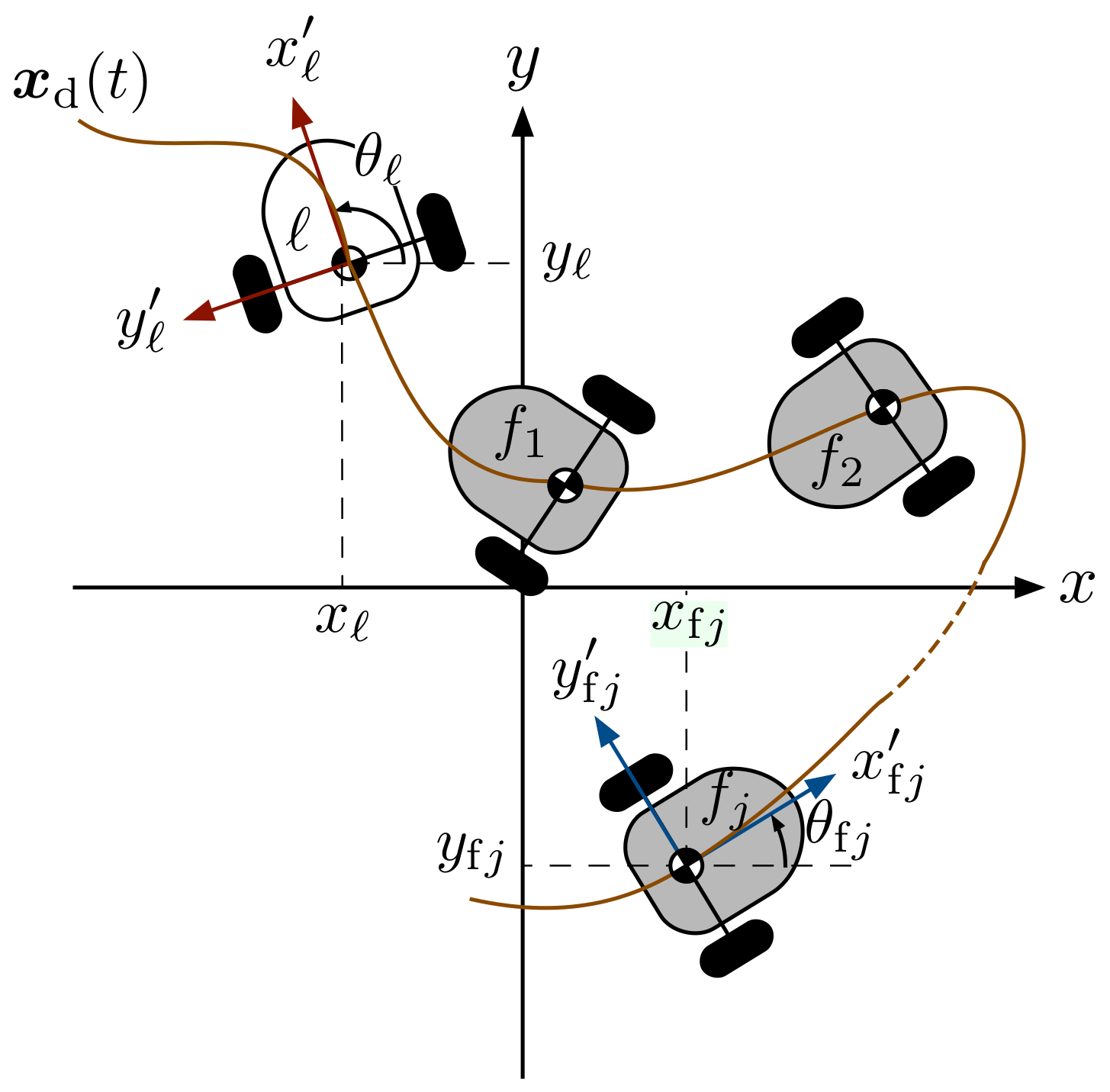
The proposed formation control strategy is based on the leader-follower approach and delayed reference signals. Contrary to the conventional distance-based leader-follower approach, where the follower robot follows the trajectory generated by the leader, in our proposed approach, the followers track the delayed desired trajectory of the leader robot. To avoid collisions, the time delay depends on the distance between the robots. The time delay becomes larger when the follower is closed to the leader and vice versa. The control objective can be stated as follows: design the control inputs ${\mathit{u}}_i$ and ${\omega }_i$ such that the position and attitude tracking errors defined as

$$\begin{array}{cc}\hfill {\tilde{\mathit{x}}}_{\ell }& ={\mathit{x}}_{\mathrm{d}}(t)-{\mathit{x}}_{\ell },{\tilde{\theta }}_{\ell }={\theta }_{\mathrm{d}\ell }(t)-{\theta }_{\ell }\hfill \end{array}$$

(18a)

$$\begin{array}{cc}\hfill {\tilde{\mathit{x}}}_{\mathrm{f}i}& ={\mathit{x}}_{\mathrm{d}}(t-{\tau }_i)-{\mathit{x}}_{\mathrm{f}i},{\tilde{\theta }}_{\mathrm{f}i}={\theta }_{\mathrm{df}i}(t-{\tau }_i)-{\theta }_{\mathrm{f}i}\hfill \end{array}$$

(18b)

converges asymptotically to zero without using attitude measurements. In (18), the subscripts ℓ and f denote the leader and follower robots and ${\mathit{x}}_{\mathrm{d}}(t)\in {\mathfrak{R}}^2$ and ${\theta }_{\mathrm{d}i}(t)$ are the desired Cartesian trajectory and desired orientation, respectively. Finally, ${\tau }_i$ denotes the time delay ($i=1,\dots ,n$) which is obtained as the output of the system

$$\begin{array}{cc}\hfill {\stackrel{·}{s}}_i& =-{\gamma }_i{s}_i+a_i(1-\exp (b_i/\parallel {\tilde{\mathit{\rho }}}_i\parallel )),s_i(0)=s_{i0}\hfill \end{array}$$

(19a)

$$\begin{array}{cc}\hfill {\tau }_i& =s_i+s_{i-1},\hfill \end{array}$$

(19b)

where $a_i$, $b_i$ and ${\gamma }_i$ are positive parameters and $s_0=0$. For the first leader we have ${\tilde{\mathit{\rho }}}_1={\mathit{x}}_{\ell }-{\mathit{x}}_{\mathrm{f}}$, and for $i>1$ we have ${\tilde{\mathit{\rho }}}_i={\mathit{x}}_{\mathrm{f}i-1}-{\mathit{x}}_{\mathrm{f}i}$. The second term in (19a) increases or decreases the magnitude of the time delay depending on the distance between the robots.

4.1. Leader Robot Controller

Before presenting the leader’s controller, let us introduce the following auxiliary error variable

$${\mathit{\eta }}_{\ell }={\tilde{\mathit{x}}}_{\ell }+{\mathit{\beta }}_{\ell }$$

(20)

where ${\mathit{\beta }}_{\ell }\in {\mathfrak{R}}^2$ is the state of the following auxiliary linear system

$$\begin{array}{cc}\hfill {\stackrel{·}{\mathit{\beta }}}_{\ell }& =-{\mathit{K}}_{\beta \ell }{\mathit{\beta }}_{\ell }-{\mathit{K}}_{\eta \ell }{\mathit{\eta }}_{\ell }\hfill \end{array}$$

(21)

where ${\mathit{K}}_{\eta \ell }={\mathit{K}}_{\eta \ell }^{\mathrm{T}}>\mathit{O}\in {\mathfrak{R}}^{2\times 2}$ and ${\mathit{K}}_{\beta \ell }={\mathit{K}}_{\beta \ell }^{\mathrm{T}}>\mathit{O}\in {\mathfrak{R}}^{2\times 2}$. Based on (20) and (21) the proposed leader’s controller is given by

$$\begin{array}{cc}\hfill {\mathit{u}}_{\ell }& ={\stackrel{·}{\mathit{x}}}_{\mathrm{d}}(t)+{\mathit{K}}_{\beta \ell }{\mathit{\beta }}_{\ell }\hfill \end{array}$$

(22a)

$$\begin{array}{cc}\hfill {\omega }_{\ell }& ={\omega }_{\mathrm{d}\ell }+k_{\mathrm{o}\ell }{\mathsf{\Theta }}_{\mathrm{d}\ell }^{\top }\mathit{S}{\widehat{\mathsf{\Theta }}}_{\ell }\hfill \end{array}$$

(22b)

where $k_{\mathrm{o}\ell }\in \mathfrak{R}$ is a positive gain, ${\widehat{\mathsf{\Theta }}}_{\ell }$ is extracted from ${\widehat{\mathit{R}}}_{\ell }$ and ${\mathsf{\Theta }}_{\mathrm{d}\ell }$ is computed according to (17). Regarding ${\omega }_{\mathrm{d}}\ell$ can be computed as

$${\omega }_{\mathrm{d}}\ell ={\mathsf{\Theta }}_{\mathrm{d}}{\ell }^{\mathrm{T}}{\mathit{S}}^{-1}{\stackrel{·}{\mathsf{\Theta }}}_{\mathrm{d}}\ell .$$

(23)

4.2. Follower Robot Controller

The next step is to design the tracking controller for the follower. The proposed position and attitude control laws for the followers have a similar structure to the leader’s controllers and are given by

$$\begin{array}{cc}\hfill {\mathit{u}}_{\mathrm{f}j}& ={\stackrel{·}{\mathit{x}}}_{\mathrm{d}}(t-{\tau }_i)+(1-{\stackrel{·}{\tau }}_i){\mathit{x}}_{\mathrm{d}}(t-{\tau }_i)+{\mathit{K}}_{\beta \mathrm{f}i}{\mathit{\beta }}_{\mathrm{f}i}\hfill \end{array}$$

(24a)

$$\begin{array}{cc}\hfill {\omega }_{\mathrm{f}i}& ={\omega }_{\mathrm{df}i}+k_{\mathrm{of}i}{\mathsf{\Theta }}_{\mathrm{df}i}^{\top }\mathit{S}{\widehat{\mathsf{\Theta }}}_{\mathrm{f}i}\hfill \end{array}$$

(24b)

where ${\mathit{K}}_{\beta \mathrm{f}i}={\mathit{K}}_{\beta \mathrm{f}i}^{\top }>\mathit{O}$, $k_{\mathrm{of}i}>0$ are the control gains and ${\mathit{\beta }}_{\mathrm{f}i}\in {\mathfrak{R}}^2$ is obtained as the solution of

$$\begin{array}{c}\hfill {\stackrel{·}{\mathit{\beta }}}_{\mathrm{f}i}=-{\mathit{K}}_{\beta \mathrm{f}i}{\mathit{\beta }}_{\mathrm{f}i}-{\mathit{K}}_{\eta \mathrm{f}i}{\mathit{\eta }}_{\mathrm{f}i}\end{array}$$

(25)

with ${\mathit{K}}_{\eta \mathrm{f}j}={\mathit{K}}_{\eta \mathrm{f}j}^{\top }>\mathit{O}$ and ${\mathit{\eta }}_{\mathrm{f}j}={\tilde{\mathit{x}}}_{\mathrm{f}j}+{\mathit{\beta }}_{\mathrm{f}j}$.

To avoid complex calculations, the time-derivative of ${\mathsf{\Theta }}_{\mathrm{d}i}$ can be approximated by a low-pass filter, ${\stackrel{·}{\mathsf{\Theta }}}_{\mathrm{d}i}={\displaystyle \frac{s}{\lambda s+1}}{\mathsf{\Theta }}_{\mathrm{d}i}$ with $\lambda >0$ is the cutoff frequency. It is important to point out that the attitude control laws (22b) and (24) does not explicitly use the orientation error ${\tilde{\theta }}_i$.

5. Stability Analysis

Once the leader and follower control laws and attitude observers have been presented we can state the following theorem which summarizes the main result of the paper.

Theorem 2.

Consider a group of nonholonomic mobile robots described by (1) in closed loop with the control laws (22) and (24) in combination with the attitude observer (8). Furthermore, assume that $|{\tilde{\theta }}_i(0)|<\pi$ and $\parallel {\stackrel{·}{\mathit{x}}}_i(t)\parallel \nrightarrow 0$ for all $t\ge 0$. Then, the leader-follower formation is achieved, i.e.,

$$\begin{array}{c}\hfill \underset{t\to \infty }{\lim }{\tilde{\mathit{x}}}_i(t)=\mathbf{0},\underset{t\to \infty }{\lim }{\tilde{\theta }}_i(t)=0\end{array}$$

with $i=\ell ,{\mathrm{f}}_j$.

Proof. 

First, we develop the closed loop dynamics of the position and attitude tracking errors. By taking into account (16a), (18), (20)–(22), (24) and (25), the position error dynamics is given by

$$\begin{array}{cc}\hfill {\stackrel{·}{\mathit{\beta }}}_i& =-{\mathit{K}}_{\beta i}{\mathit{\beta }}_i-{\mathit{K}}_{\eta i}{\mathit{\eta }}_i\hfill \end{array}$$

(26)

$$\begin{array}{cc}\hfill {\stackrel{·}{\mathit{\eta }}}_i& =-{\mathit{K}}_{\eta i}{\mathit{\eta }}_i-{\nu }_i\left({\mathsf{\Theta }}_i-{\mathsf{\Theta }}_{\mathrm{d}i}\right).\hfill \end{array}$$

(27)

By using trigonometric identities, the term ${\nu }_i\left({\mathsf{\Theta }}_i-{\mathsf{\Theta }}_{\mathrm{d}i}\right)$ can be written as

$${\nu }_i\left({\mathsf{\Theta }}_i-{\mathsf{\Theta }}_{\mathrm{d}i}\right)={\mathit{\psi }}_i(t,{\tilde{\theta }}_i){\tilde{\theta }}_i={\nu }_i{\mathit{R}}_i\left[\begin{array}{c}(1-\cos ({\tilde{\theta }}_i))/{\tilde{\theta }}_i\\ -\sin ({\tilde{\theta }}_i)/{\tilde{\theta }}_i\end{array}\right]{\tilde{\theta }}_i.$$

(28)

On the other hand, by taking into account the attitude observer (8) and attitude control laws (22b) and (24b), the attitude error dynamics is given by

$$\begin{array}{cc}\hfill {\stackrel{·}{\stackrel{~}{\theta }}}_i& =-k_{\mathrm{o}i}\sin ({\tilde{\theta }}_i)+k_{\mathrm{o}i}{\mathsf{\Theta }}_{\mathrm{d}i}^{\top }{\mathit{S}\mathit{R}}_i(\mathit{I}-{\tilde{\mathit{R}}}_i^{\top }){\mathit{e}}_1\hfill \end{array}$$

(29)

$$\begin{array}{cc}\hfill {\stackrel{·}{\stackrel{~}{\mathit{R}}}}_i& =({\omega }_i-{\widehat{\omega }}_i){\tilde{\mathit{R}}}_i\mathit{S}\hfill \end{array}$$

(30)

where the equalities ${\mathsf{\Theta }}_{\mathrm{d}i}^{\top }\mathit{S}{\mathsf{\Theta }}_i=\sin ({\tilde{\theta }}_i)$ and ${\mathsf{\Theta }}_i-{\widehat{\mathsf{\Theta }}}_i={\mathit{R}}_i(\mathit{I}-{\tilde{\mathit{R}}}_i^{\top }){\mathit{e}}_1$ have been used.

Finally, by defining ${\mathit{z}}_i={\left[\begin{array}{cc}{\mathit{\beta }}_i^{\top }& {\mathit{\eta }}_i^{\top }\end{array}\right]}^{\top }\in {\mathfrak{R}}^4$ the whole closed-loop dynamics can be written as follows

$$\begin{array}{cc}\hfill {\mathsf{\Sigma }}_1:& \left\{{\stackrel{·}{\mathit{z}}}_i={\mathit{A}}_i{\mathit{z}}_i+{\mathsf{\Psi }}_i(t,{\tilde{\theta }}_i){\tilde{\theta }}_i\right.\hfill \end{array}$$

(31a)

$${\mathsf{\Sigma }}_2:\left\{\begin{array}{cc}{\stackrel{·}{\stackrel{~}{\theta }}}_i=& -k_{\mathrm{o}i}\sin ({\tilde{\theta }}_i)+k_{\mathrm{o}i}{\mathsf{\Theta }}_{\mathrm{d}i}^{\top }{\mathit{S}\mathit{R}}_i(\mathit{I}-{\tilde{\mathit{R}}}_i^{\top }){\mathit{e}}_1\hfill \\ {\stackrel{·}{\stackrel{~}{\mathit{R}}}}_i=& ({\omega }_i-{\widehat{\omega }}_i){\tilde{\mathit{R}}}_i\mathit{S}\hfill \end{array}\right.$$

(31b)

where

$${\mathit{A}}_i=\left[\begin{array}{cc}-{\mathit{K}}_{\beta i}& -{\mathit{K}}_{\eta i}\\ \mathit{O}& -{\mathit{K}}_{\eta i}\end{array}\right],{\mathsf{\Psi }}_i(t,{\tilde{\theta }}_i)=\left[\begin{array}{c}\mathbf{0}\\ {\mathit{\psi }}_i(t,{\tilde{\theta }}_i)\end{array}\right].$$

Clearly, the complete closed-loop system presents a cascade structure between the position and attitude error dynamics. If ${\tilde{\mathit{R}}}_i=\mathit{I}$, then, ${\widehat{\mathit{R}}}_i={\mathit{R}}_i$ which implies that ${\widehat{\mathsf{\Theta }}}_i={\mathsf{\Theta }}_i$. In this case, the term ${\omega }_i-{\widehat{\omega }}_i$ becomes

$${\omega }_i-{\widehat{\omega }}_i=k_{\mathrm{a}i}{\mathit{v}}_i^{\top }\mathit{S}{\mathsf{\Theta }}_i=\frac{k_{\mathrm{a}i}}{\parallel {\stackrel{·}{\mathit{x}}}_i\parallel }{\stackrel{·}{\mathit{x}}}_i^{\top }\mathit{S}{\mathsf{\Theta }}_i=0\Rightarrow \stackrel{·}{\stackrel{~}{\mathit{R}}}=\mathit{O}$$

The result follows from the nonholonomic constrain (2). The previous result shows that the equilibrium point of (31) is $({\mathit{z}}_i^{\star },{\tilde{\theta }}_i^{\star },{\mathit{R}}_i^{\star })=(\mathbf{0},k\pi ,\mathit{I})$ with $k=0,1,2,\dots$.

Now let us analyze the subsystem ${\mathsf{\Sigma }}_2$ which is independent of the state ${\mathit{z}}_i$ and has a cascade structure with $k_{\mathrm{o}i}{\mathsf{\Theta }}_{\mathrm{d}i}^{\top }{\mathit{S}\mathit{R}}_i(\mathit{I}-{\tilde{\mathit{R}}}_i^{\top }){\mathit{e}}_1$ as an interconnection term. This term is bounded and according to Theorem 1 vanishes since the attitude observer error ${\tilde{\mathit{R}}}_i\to \mathit{I}$ as $t\to \infty$. Moreover, the equilibrium point ${\tilde{\theta }}_i=0$ of the unperturbed system

$${\stackrel{·}{\stackrel{~}{\theta }}}_i=-k_{\mathrm{o}i}\sin ({\tilde{\theta }}_i)$$

(32)

is locally asymptotically stable with Lyapunov function $V_{\theta i}=1-\cos ({\tilde{\theta }}_i)$∀${\tilde{\theta }}_i\in (-\pi ,\pi )$. Furthermore, ${\tilde{\theta }}_i=0$ is locally exponentially stable since the linear approximation of (32) is given by ${\stackrel{·}{\stackrel{~}{\theta }}}_i=-k_{\mathrm{o}i}{\tilde{\theta }}_i$. Therefore, according with Lemma A1 (see Appendix A) the subsystem ${\stackrel{·}{\stackrel{~}{\theta }}}_i=-k_{\mathrm{o}i}\sin ({\tilde{\theta }}_i)+k_{\mathrm{o}i}{\mathsf{\Theta }}_{\mathrm{d}i}^{\top }{\mathit{S}\mathit{R}}_i(\mathit{I}-{\tilde{\mathit{R}}}_i^{\top }){\mathit{e}}_1$ is Input-to-State Stable (ISS) with input $(\mathit{I}-{\tilde{\mathit{R}}}_i^{\top }){\mathit{e}}_1$. Clearly, the attitude subsystem ${\mathsf{\Sigma }}_2$ satisfies the condition of Theorem A1 given in Appendix A, thus, it is concluded that the equilibrium point $({\tilde{\theta }}_i,{\tilde{\mathit{R}}}_i)=(0,\mathit{I})$ is uniformly asymptotically stable.

The position subsystem ${\mathsf{\Sigma }}_1$ can be analyzed using similar arguments. It is straightforward to show that the matrix ${\mathit{A}}_i$ is Hurwitz. Therefore, the equilibrium point ${\mathit{z}}_i=\mathbf{0}$ of the unforced subsystem ${\stackrel{·}{\mathit{z}}}_i={\mathit{A}}_i{\mathit{z}}_i$ (with ${\tilde{\theta }}_i=0$) is exponentially stable. This implies that the subsystem ${\mathsf{\Sigma }}_1$ is ISS with input ${\tilde{\theta }}_i$. The closed loop system ${\mathsf{\Sigma }}_1$ and ${\mathsf{\Sigma }}_2$ satisfy the conditions of Theorem A1. As a result, it is concluded that $({\mathit{z}}_i,{\tilde{\theta }}_i,{\tilde{\mathit{R}}}_i)\to (\mathbf{0},0,\mathit{I})$ as $t\to \infty$. The convergence of ${\mathit{z}}_i$ to zero implies that ${\mathit{\eta }}_i$ and ${\mathit{\beta }}_i$ also converge asymptotically to zero. Then, it follows that the position tracking error ${\tilde{\mathit{x}}}_i={\mathit{\eta }}_i+{\mathit{\beta }}_i\to \mathbf{0}$ as $t\to \infty$. This completes the proof. □

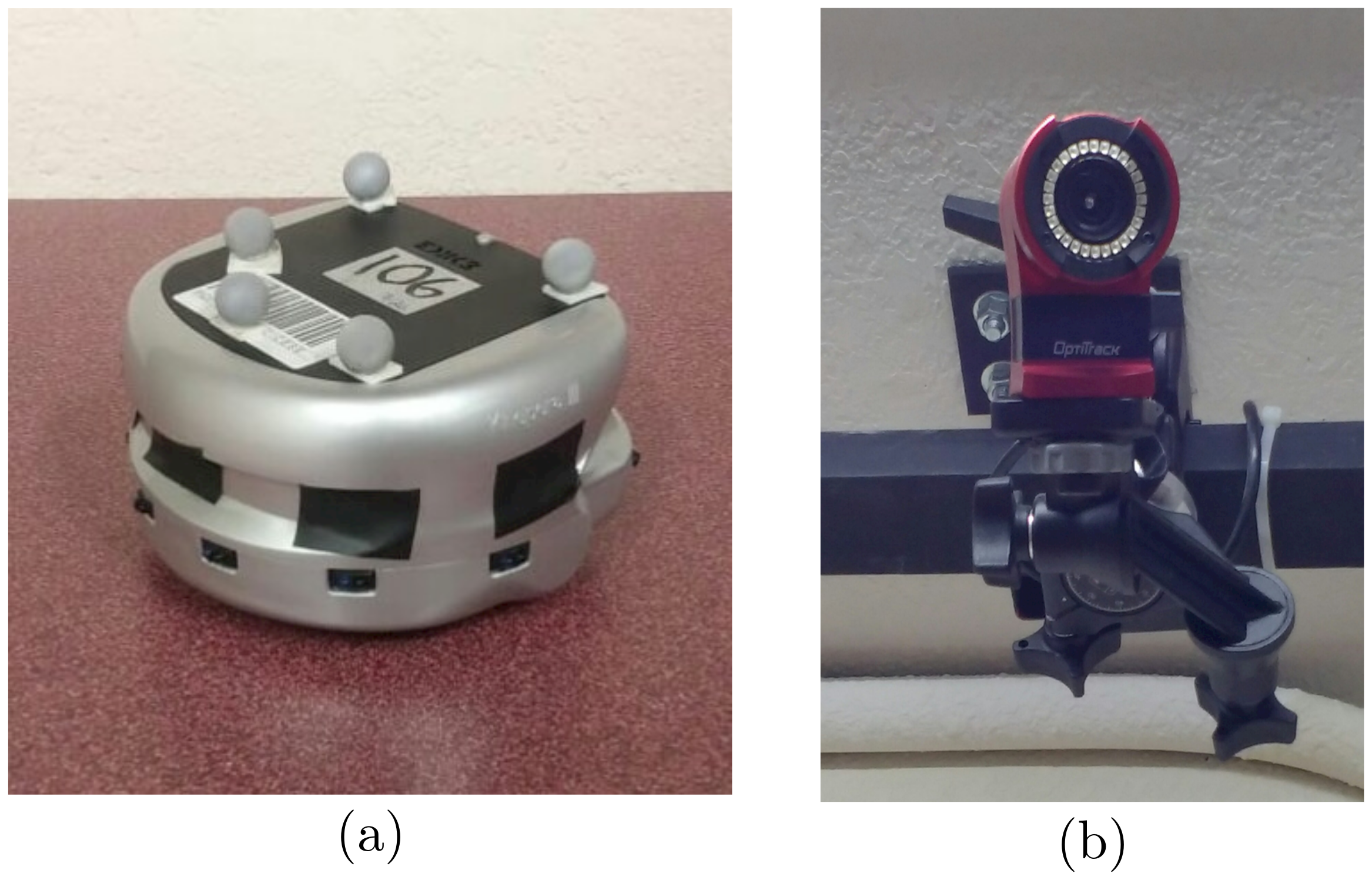
6. Experimental Results

In this section, experimental results are presented to validate the performance of the attitude observer and control laws developed in Section 3 and Section 4. The testbed is composed of three Khepera III mobile robots from K-Team and six infrared Optitrack cameras which measure the Cartesian position of the robots (see Figure 2). Although the infrared cameras can also measure the orientation of the robot, This measurement is used only for comparison purposes and do not influence the behavior of the controller. The control laws and the observer were programmed in Matlab with a sample time of 20 [ms]. The control signals were sent to the robots via WIFI communication channel.

Table 1. Observer, controller gains and delay parameters.

Robot	${\mathit{k}}_{\mathbf{a}\mathit{i}}$	${\mathit{K}}_{\mathit{\eta }\mathit{i}}$	${\mathit{K}}_{\mathit{\beta }\mathit{i}}$	${\mathit{b}}_{\mathit{i}}$	${\mathit{\gamma }}_{\mathit{i}}$	${\mathit{\lambda }}_{\mathit{i}}$	${\mathit{\kappa }}_{\mathit{i}}$	${\mathit{\zeta }}_{\mathit{i}}$
Leader	3	$4\mathit{I}$	$3.5\mathit{I}$	-	-	10	$20\mathit{I}$	$5\mathit{I}$
Follower 1	3	$4\mathit{I}$	$3.5\mathit{I}$	1	1	10	$20\mathit{I}$	$5\mathit{I}$
Follower 2	3	$4\mathit{I}$	$3.5\mathit{I}$	1	1	10	$20\mathit{I}$	$5\mathit{I}$

summarizes the parameter values of the control law and the orientation observer employed in the experiments. It is worth to notice, that the initial postures of the robots are selected arbitrarily in every case.

The control algorithms together with the attitude observer were tested using two desired trajectories, a circular path and a lemniscate curve. The parametric equations of both desired trajectories are shown below

$${\mathit{x}}_{{\mathrm{dm}}_1}=\left[\begin{array}{c}0.3\cos \left({\displaystyle \frac{\pi }{15}t}\right)\\ 0.3\sin \left({\displaystyle \frac{\pi }{15}t}\right)\end{array}\right][\mathrm{m}],{\mathit{x}}_{{\mathrm{dm}}_2}=\left[\begin{array}{c}0.35\sin \left({\displaystyle \frac{2\pi }{45}t}\right)\\ 0.35\sin \left({\displaystyle \frac{4\pi }{45}t}\right)\end{array}\right][\mathrm{m}]$$

(33)

The Cartesian velocity ${\stackrel{·}{\mathit{x}}}_i$ can be computed by means of numerical differentiation. However, we obtained better results with the following velocity observer [27]

$$\begin{array}{cc}\hfill {\stackrel{·}{\widehat{\mathit{x}}}}_i& ={\mathit{\kappa }}_i({\mathit{x}}_i-{\widehat{\mathit{x}}}_i)+{\mathit{\mu }}_i\hfill \\ \hfill {\stackrel{·}{\mathit{\mu }}}_i& ={\mathit{\zeta }}_i({\mathit{x}}_i-{\widehat{\mathit{x}}}_i)\hfill \end{array}$$

where ${\mathit{\kappa }}_i$, ${\mathit{\zeta }}_i\in {\mathfrak{R}}^{2\times 2}$ are positive definite matrices and ${\widehat{\mathit{x}}}_i\in {\mathfrak{R}}^2$ is an estimate of the Cartesian position ${\mathit{x}}_i$.

The observer, controller gains and the parameters of the delay dynamic equation are shown in Table 1. Regarding the parameter $a_{\mathrm{j}}$, for the first trajectory was set to $a_1=3$ and for the second one we have $a_2=5$. All other parameters were the same for both trajectories.

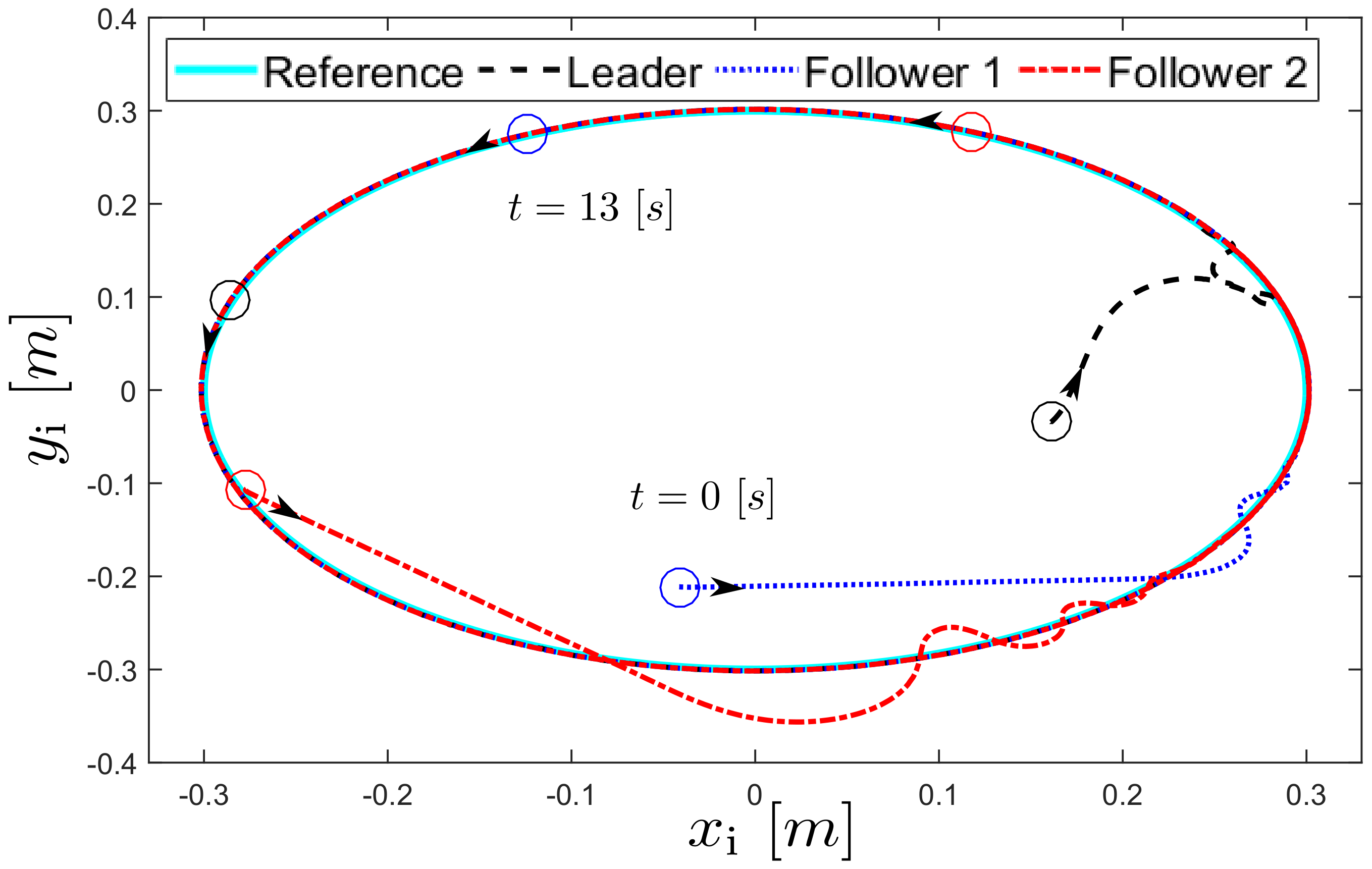
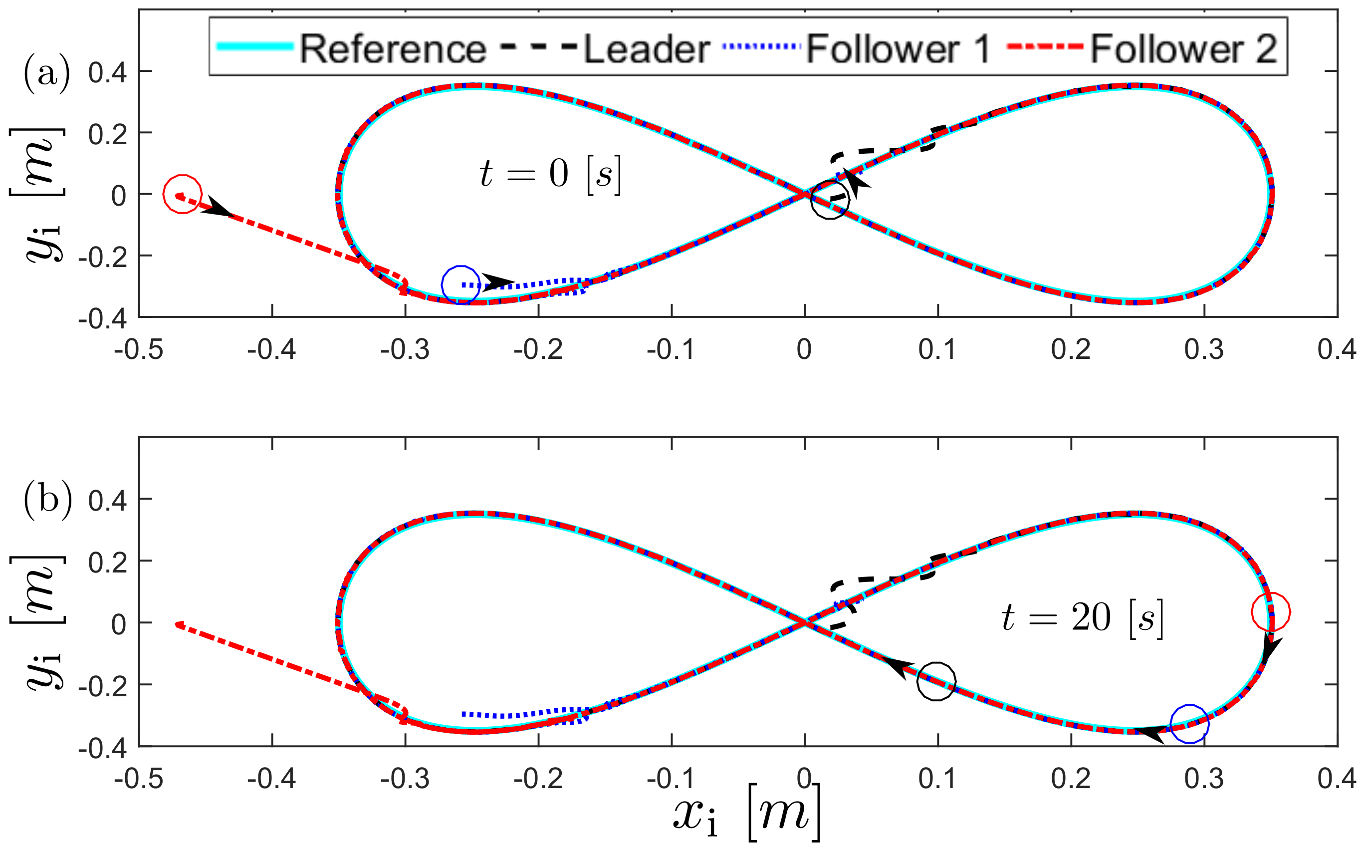
The trajectories of the robots obtained during the two experiments with the desired Cartesian trajectories are shown in Figure 3 and Figure 4, respectively. The figures also shown the robots’ positions at the time instants $t=0$ [s], $t=13$ [s] for the first experiment and $t=0$ [s] and $t=20$ [s] for the second experiment. In both cases, after the transient response the robots successfully achieve the convoy formation.

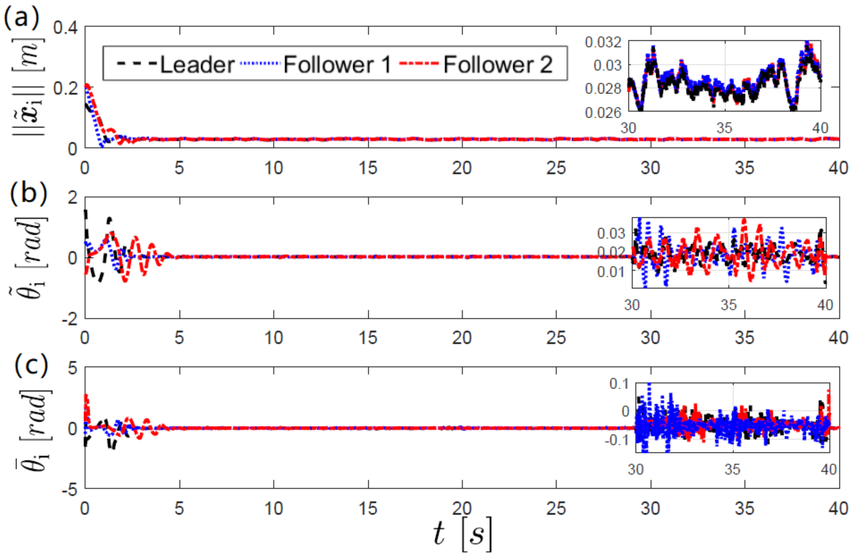
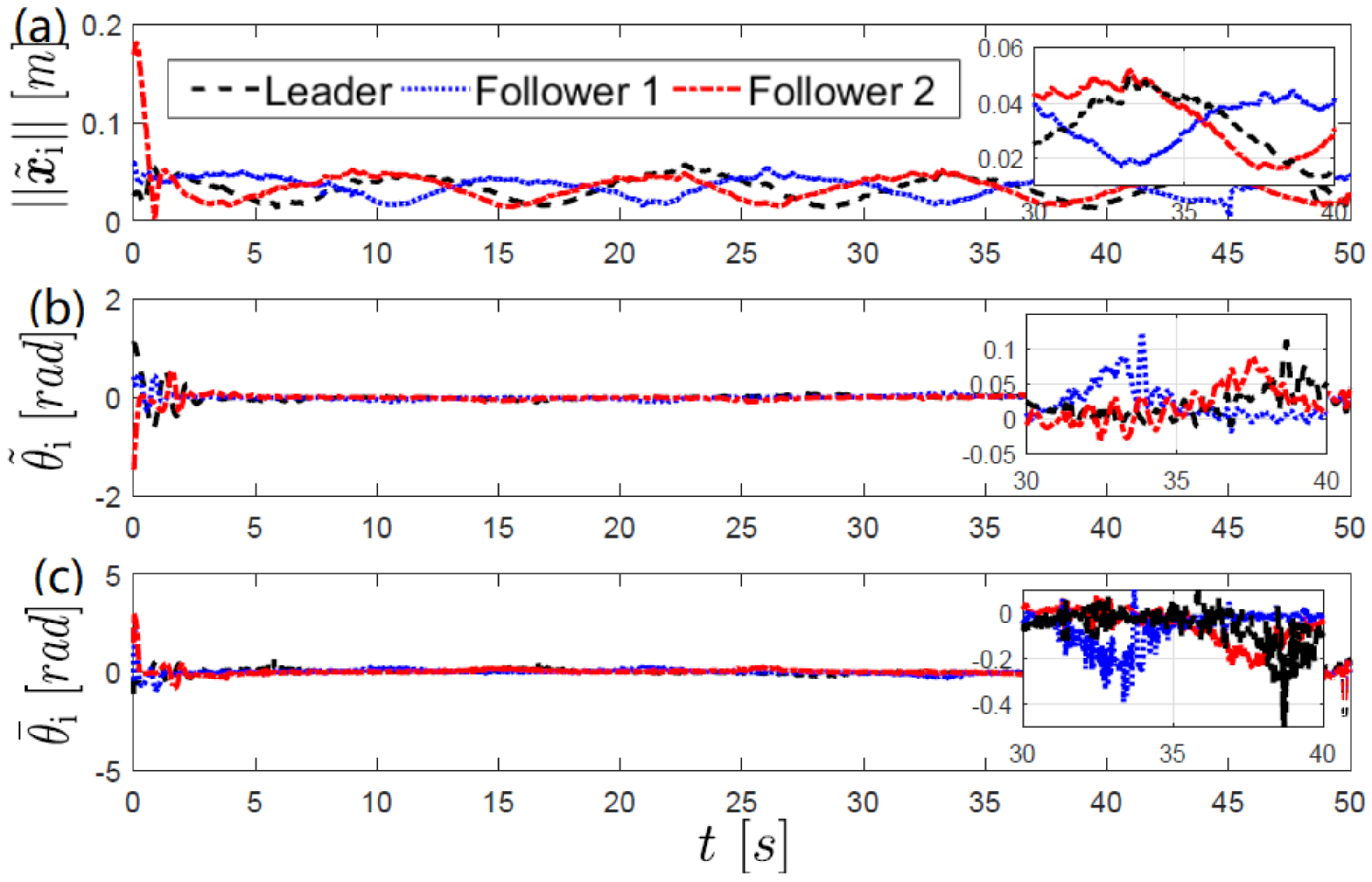
In order to assess the performance of the attitude observer and control laws we compute the orientation errors ${\tilde{\theta }}_i={\theta }_i-{\theta }_{\mathrm{d}i}$ and ${\overline{\theta }}_i={\theta }_i-{\widehat{\theta }}_i$ where ${\theta }_i$ is the angle measured by the cameras and the estimated angle ${\widehat{\theta }}_i$ is extracted from ${\widehat{\mathsf{\Theta }}}_i$ as follows

$$\begin{array}{c}\hfill {\widehat{\theta }}_i=\mathrm{atan}2({\widehat{\Theta }}_{2i},{\widehat{\Theta }}_{1i})\end{array}$$

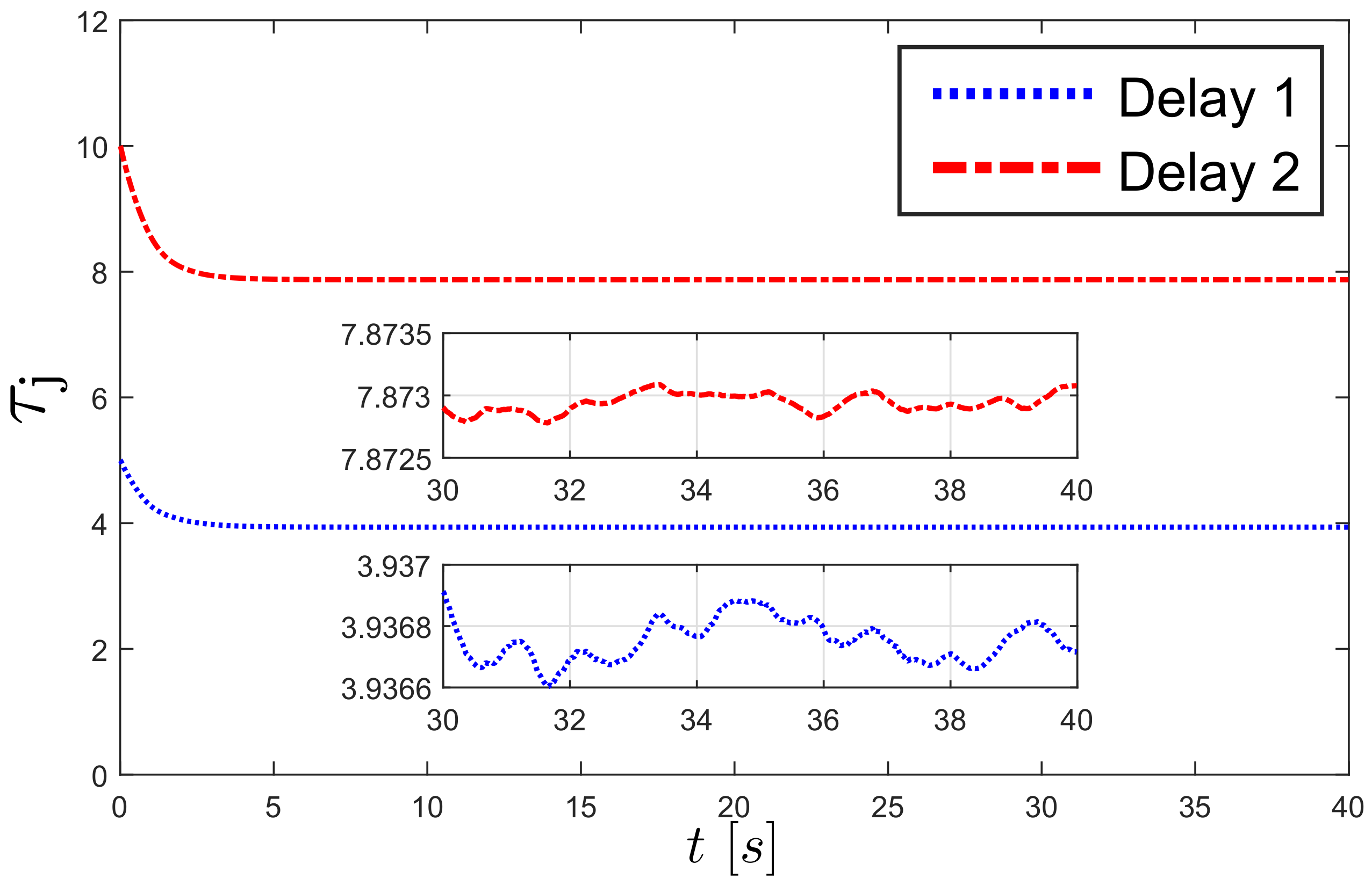
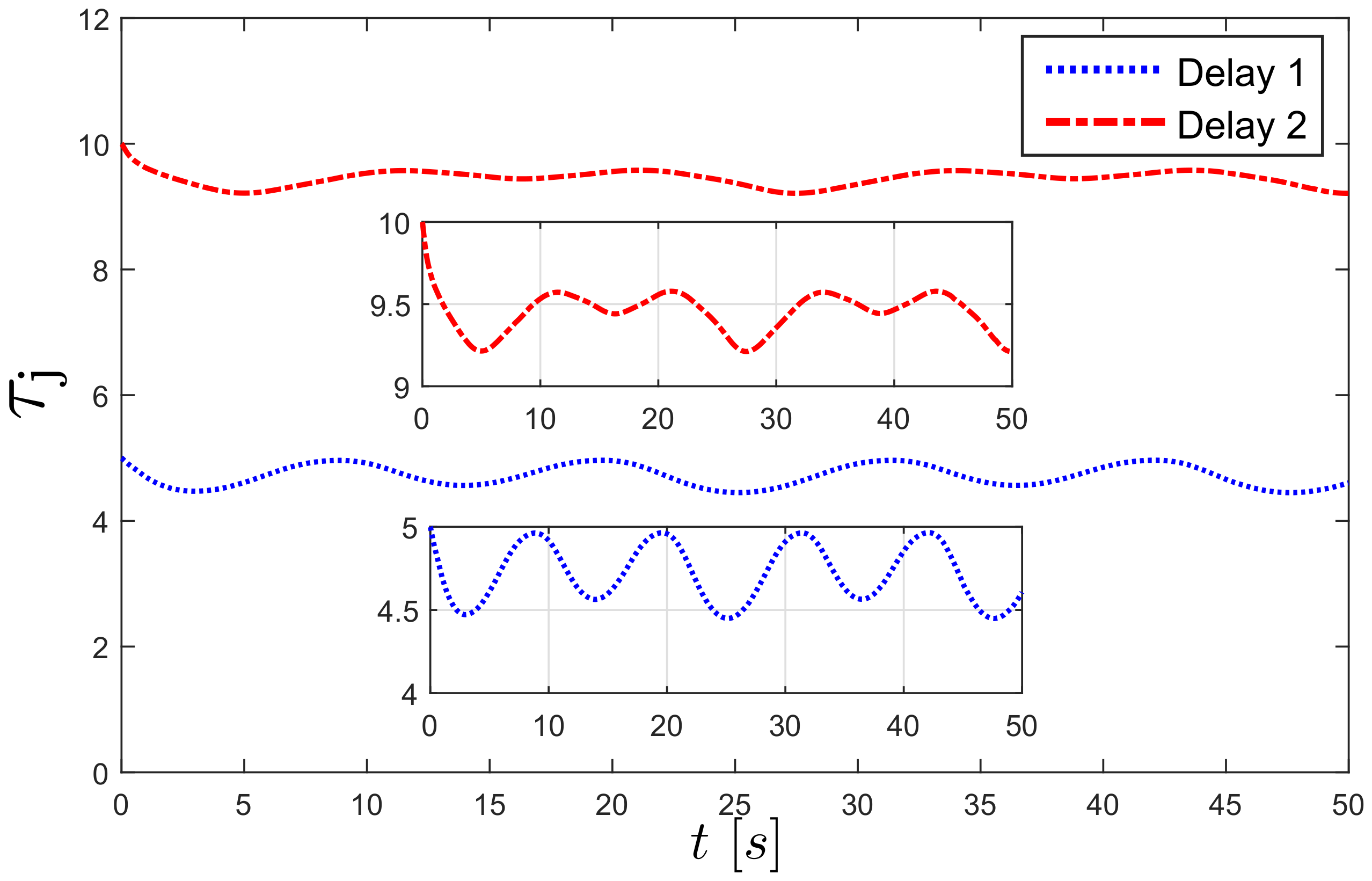
where $\mathrm{atan}2(·,·)$ is the two argument arctangent function and ${\widehat{\mathsf{\Theta }}}_i=\mathrm{col}({\widehat{\mathsf{\Theta }}}_{1i},{\widehat{\mathsf{\Theta }}}_{2i})$. The time evolution of the position and attitude tracking errors obtained in each experiment are shown in Figure 5 and Figure 6. It is observed in the Figures that despite the unmodeled dynamics and discretization of the control laws, a good tracking was achieved. The time evolution of the time delays are shown in Figure 7 and Figure 8. Notice that for the circular path the delays converge to a constant value while for the second trajectory the time delays change slowly while their magnitude increases at the points of the curve with greater curvature (see Figure 4b). This behavior was expected since at this points the robots come closer to each other.

In order to assess the performance of the proposed algorithm, the RMS error is computed for the distance and orientation of each robot to its desired trajectory, additionally to the RMS error of the estimation of the orientation observer is presented.

Table 2. RMS errors of distance, orientation and observed orientation of the robots in the circular trajectory experiment.

Robot	Distance [m]	Orientation [rad]	Observation [rad]
Leader	0.0330	0.1533	0.2115
Follower 1	0.0336	0.0806	0.1217
Follower 2	0.0367	0.1416	0.1949

collects the results for the circular desired trajectory while

Table 3. RMS errors of distance, orientation and observed orientation of the robots in the lemniscate trajectory experiment.

Robot	Distance [m]	Orientation [rad]	Observation [rad]
Leader	0.0360	0.1221	0.1814
Follower 1	0.0365	0.0654	0.1862
Follower 2	0.0397	0.0775	0.2060

shows the results corresponding to the lemniscate curve desired trajectory experiment. On both cases it is observed that the RMS distance error is bellow 0.04 m, while RMS orientation error is under 0.155 radians.

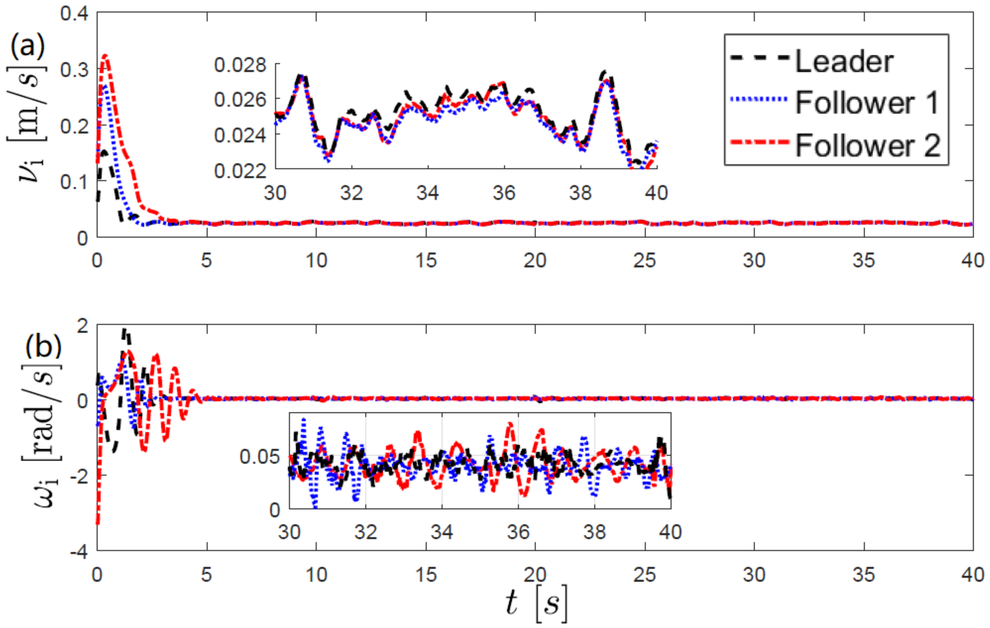
Finally, Figure 9 and Figure 10 show the control inputs. Notice that ${\nu }_i(t)\nrightarrow 0$ for all $t\ge 0$ this implies that the assumption $\parallel {\stackrel{·}{\mathit{x}}}_i(t)\parallel \nrightarrow 0$ is satisfied in both experiments.

7. Conclusions

In this paper, we proposed kinematic control laws in combination with an attitude observer that solve the problem of convoy formation for a group of nonholonomic mobile robots without using attitude measurements. The proposed control approach is based on the leader-follower scheme but contrary to other works, we used delayed reference signals for the follower robots. The time delays depend on the distance between the robots and are obtained as the outputs of a dynamical system that couples the leader and follower dynamics. As result, collisions between the members of the group are avoided. The kinematic control laws were designed by exploiting the cascade structure of the robots’ kinematic model. The proposed controllers are decentralized since only require its own position and the position of the nearest leader. On the other hand, the attitude observer was designed directly on $SO(2)$ and it can be used in open and closed loop schemes. Finally, real-time experiments are presented to show the effectiveness of the proposed control-observer approach.

References

1. Spletzer, J.; Das, A.K.; Fierro, R.; Taylor, C.J.; Kumar, V.; Ostrowski, J.P. Cooperative localization and control for multi-robot manipulation. In Proceedings of the 2001 IEEE/RSJ International Conference on Intelligent Robots and Systems. Expanding the Societal Role of Robotics in the the Next Millennium (Cat. No. 01CH37180), Maui, HI, USA, 29 October–3 November 2001; IEEE: New York, NY, USA, 2001; Volume 2, pp. 631–636. [Google Scholar]
2. Hosseinzadeh, M. UAV geofencing: Navigation of UVAs in constrained environments. In Unmanned Aerial Systems; Elsevier: Amsterdam, The Netherlands, 2021; pp. 567–594. [Google Scholar]
3. Parker, L.E. Current state of the art in distributed autonomous mobile robotics. In Distributed Autonomous Robotic Systems 4; Springer: Berlin/Heidelberg, Germany, 2000; pp. 3–12. [Google Scholar]
4. Dai, S.L.; He, S.; Chen, X.; Jin, X. Adaptive Leader-Follower Formation Control of Nonholonomic Mobile Robots With Prescribed Transient and Steady-State Performance. IEEE Trans. Ind. Inform. 2019, 16, 3662–3671. [Google Scholar] [CrossRef]
5. Cui, R.; Ge, S.S.; How, B.V.E.; Choo, Y.S. Leader—Follower formation control of underactuated autonomous underwater vehicles. Ocean Eng. 2010, 37, 1491–1502. [Google Scholar] [CrossRef]
6. Sands, T. Development of Deterministic Artificial Intelligence for Unmanned Underwater Vehicles (UUV). J. Mar. Sci. Eng. 2020, 8, 578. [Google Scholar] [CrossRef]
7. Turpin, M.; Michael, N.; Kumar, V. Decentralized formation control with variable shapes for aerial robots. In Proceedings of the 2012 IEEE International Conference on ROBOTICS and Automation, Saint Paul, MN, USA, 14–18 May 2012; IEEE: New York, NY, USA, 2012; pp. 23–30. [Google Scholar]
8. Do, K.; Pan, J. Nonlinear formation control of unicycle-type mobile robots. Robot. Auton. Syst. 2007, 55, 191–204. [Google Scholar] [CrossRef]
9. Coquet, C.; Arnold, A.; Bouvet, P.J. Control of a Robotic Swarm Formation to Track a Dynamic Target with Communication Constraints: Analysis and Simulation. Appl. Sci. 2021, 11, 3179. [Google Scholar] [CrossRef]
10. Beard, R.W.; Lawton, J.; Hadaegh, F.Y. A coordination architecture for spacecraft formation control. IEEE Trans. Control Syst. Technol. 2001, 9, 777–790. [Google Scholar] [CrossRef] [Green Version]
11. Chen, J.; Sun, D.; Yang, J.; Chen, H. Leader-follower formation control of multiple non-holonomic mobile robots incorporating a receding-horizon scheme. Int. J. Robot. Res. 2010, 29, 727–747. [Google Scholar] [CrossRef]
12. Martínez-Clark, R.; Cruz-Hernández, C.; Pliego-Jimenez, J.; Arellano-Delgado, A. Control algorithms for the emergence of self-organized behaviours in swarms of differential-traction wheeled mobile robots. Int. J. Adv. Robot. Syst. 2018, 15, 1729881418806435. [Google Scholar] [CrossRef]
13. Balch, T.; Arkin, R.C. Behavior-based formation control for multirobot teams. IEEE Trans. Robot. Autom. 1998, 14, 926–939. [Google Scholar] [CrossRef] [Green Version]
14. Wang, X.; Li, S.; Shi, P. Distributed finite-time containment control for double-integrator multiagent systems. IEEE Trans. Cybern. 2013, 44, 1518–1528. [Google Scholar] [CrossRef] [PubMed] [Green Version]
15. Yang, Z.; Zhu, S.; Chen, C.; Feng, G.; Guan, X. Leader-follower formation control of nonholonomic mobile robots with bearing-only measurements. J. Frankl. Inst. 2020, 357, 1628–1643. [Google Scholar] [CrossRef]
16. Xiao, H.; Li, Z.; Chen, C.P. Formation control of leader–follower mobile robots’ systems using model predictive control based on neural-dynamic optimization. IEEE Trans. Ind. Electron. 2016, 63, 5752–5762. [Google Scholar] [CrossRef]
17. Sun, D.; Wang, C.; Shang, W.; Feng, G. A synchronization approach to trajectory tracking of multiple mobile robots while maintaining time-varying formations. IEEE Trans. Robot. 2009, 25, 1074–1086. [Google Scholar]
18. Lewis, M.A.; Tan, K.H. High precision formation control of mobile robots using virtual structures. Auton. Robot. 1997, 4, 387–403. [Google Scholar] [CrossRef]
19. Besseghieur, K.L.; Trkebiski, R.; Kaczmarek, W.; Panasiuk, J. Leader-follower formation control for a group of ROS-enabled mobile robots. In Proceedings of the 2019 6th International Conference on Control, Decision and Information Technologies (CoDIT), Paris, France, 23–26 April 2019; IEEE: New York, NY, USA, 2019; pp. 1556–1561. [Google Scholar]
20. Halima, M.; Abdelouahab, H.; Yaakoub, T.M. Leader-follower formation control using PI controller. In Proceedings of the 2018 International Conference on Electrical Sciences and Technologies in Maghreb (CISTEM), Algiers, Algeria, 28–31 October 2018; IEEE: New York, NY, USA, 2018; pp. 1–4. [Google Scholar]
21. Bayuwindra, A.; Lefeber, E.; Ploeg, J.; Nijmeijer, H. Extended Look-Ahead Tracking Controller With Orientation-Error Observer for Vehicle Platooning. IEEE Trans. Intell. Transp. Syst. 2019, 21, 4808–4821. [Google Scholar] [CrossRef]
22. Liang, X.; Wang, H.; Liu, Y.H.; Chen, W.; Liu, T. Formation control of nonholonomic mobile robots without position and velocity measurements. IEEE Trans. Robot. 2017, 34, 434–446. [Google Scholar] [CrossRef]
23. Pliego-Jiménez, J.; Martínez-Clark, R.; Cruz-Hernández, C. Orientation and velocity observers for unicycle mobile robots. In Proceedings of the 2019 18th European Control Conference (ECC), Naples, Italy, 25–28 June 2019; IEEE: New York, NY, USA, 2019; pp. 2134–2139. [Google Scholar]
24. Noijen, S.P.M.; Lambrechts, P.F.; Nijmeijer, H. An observer-controller combination for a unicycle mobile robot. Int. J. Control 2005, 78, 81–87. [Google Scholar] [CrossRef] [Green Version]
25. Asif, M.; Memon, A.Y.; Junaid Khan, M. Output feedback control for trajectory tracking of wheeled mobile robot. Intell. Autom. Soft Comput. 2016, 22, 75–87. [Google Scholar] [CrossRef]
26. Mahony, R.; Hamel, T.; Pflimlin, J.M. Nonlinear complementary filters on the special orthogonal group. IEEE Trans. Autom. Control 2008, 53, 1203–1218. [Google Scholar] [CrossRef] [Green Version]
27. Pliego-Jiménez, J.; Arteaga-Pérez, M. Telemanipulation of cooperative robots: A case of study. Int. J. Control 2018, 91, 1284–1299. [Google Scholar] [CrossRef]
28. Khalil, H. Nonlinear Systems; Prentice Hall: Hoboken, NJ, USA, 1996. [Google Scholar]
Figure 1. A group of nonholonomic mobile robots with one leader and n followers.
Applsci 11 05639 g001
Figure 2. Experimental testbed: (a) Differential drive Khepera III mobile robot, and (b) Optitrack infrared camera.
Applsci 11 05639 g002
Figure 3. Trajectory of the robot group following the circular path: Robots at the time instants t = 0 and t = 15 s.
Applsci 11 05639 g003
Figure 4. Trajectory of the robot group following the lemniscate curve: (a) Robots at t = 0 s, and (b) Robots at t = 30 s.
Applsci 11 05639 g004
Figure 5. Time evolution of the position and attitude errors in the first experiment (circular path): (a) Norm of the position error x ~ i , (b) orientation error θ ~ i = θ d i θ i , (c) observation error θ ¯ i = θ i θ ^ i .
Applsci 11 05639 g005
Figure 6. Time evolution of the position and attitude errors in the second experiment (lemniscate curve): (a) Norm of the position error x ~ i , (b) orientation error θ ~ i = θ d i θ i , (c) observation error θ ¯ i = θ i θ ^ i .
Applsci 11 05639 g006
Figure 7. Time evolution of the delay for the first trajectory.
Applsci 11 05639 g007
Figure 8. Time evolution of the delay for the second trajectory.
Applsci 11 05639 g008
Figure 9. Control inputs obtained in the first experiment: (a) ν i , (b) ω i .
Applsci 11 05639 g009
Figure 10. Control inputs obtained in the second experiment: (a) ν i , (b) ω i .
Applsci 11 05639 g010