Article

Intrusion Detection Based on Gray-Level Co-Occurrence Matrix and 2D Dispersion Entropy

by
Gianmarco Baldini
1,*,
Jose Luis Hernandez Ramos
1 and
Irene Amerini
2
1
European Commission, Joint Research Centre, 21027 Ispra, Italy
2
Department of Computer, Control and Management Engineering A. Ruberti, Sapienza University of Rome, 00185 Rome, Italy
*
Author to whom correspondence should be addressed.
Appl. Sci. 2021, 11(12), 5567; https://doi.org/10.3390/app11125567
Submission received: 20 April 2021 / Revised: 25 May 2021 / Accepted: 11 June 2021 / Published: 16 June 2021
(This article belongs to the Special Issue Cryptography and Its Applications in Information Security)

Abstract

:
The Intrusion Detection System (IDS) is an important tool to mitigate cybersecurity threats in an Information and Communication Technology (ICT) infrastructure. The function of the IDS is to detect an intrusion to an ICT system or network so that adequate countermeasures can be adopted. Desirable features of IDS are computing efficiency and high intrusion detection accuracy. This paper proposes a new anomaly detection algorithm for IDS, where a machine learning algorithm is applied to detect deviations from legitimate traffic, which may indicate an intrusion. To improve computing efficiency, a sliding window approach is applied where the analysis is applied on large sequences of network flows statistics. This paper proposes a novel approach based on the transformation of the network flows statistics to gray images on which Gray level Co-occurrence Matrix (GLCM) are applied together with an entropy measure recently proposed in literature: the 2D Dispersion Entropy. This approach is applied to the recently public IDS data set CIC-IDS2017. The results show that the proposed approach is competitive in comparison to other approaches proposed in literature on the same data set. The approach is applied to two attacks of the CIC-IDS2017 data set: DDoS and Port Scan achieving respectively an Error Rate of 0.0016 and 0.0048.

1. Introduction

Our society is becoming increasingly dependent on the internet and communication services but the risk of cybersecurity threats has also increased. Intrusion Detection System (IDS) can be a powerful tool to mitigate cybersecurity attacks. Research in IDS is more than 20 years old and various types of IDS have been proposed in literature: signature-based IDS, which focuses on the recognition of traffic patterns associated to a threat, anomaly-based IDS which detects deviations from a model of legitimate traffic and often relies on machine learning or reputation-based IDS based on the calculation of reputation scores [1]. Requirements or preferred features of IDS have been already defined in literature [1,2] and they can be summarized in: (a) fast detection of the attack, (b) high detection accuracy and (c) low computing complexity of the detection algorithm to support the capability to analyze a large amount of traffic due to the high throughput of the current networks. The successful fulfillment of these three main requirements can be challenging because there are trade-offs between them. For example, algorithms, which are able to obtain high detection accuracy, may require considerable computing resources or they may not be able to achieve a fast detection. The advantage of anomaly-based IDS, in comparison to signature-based IDS, is to potential detect new attacks which have not been recorded before and where the corresponding signature has not been created yet. On the other side, the detection of anomalies in high throughput traffic would benefit from dimensionality reduction while preserving an high detection accuracy. To achieve this goal, anomaly-based IDS have been proposed in literature where a sliding window is used [2,3].
This paper focuses on an anomaly detection approach where the network flows data is collected in windows of fixed size, which are then converted to gray images on which the Gray level Co-occurrence Matrix (GLCM) is calculated. Then, the features (e.g., contrast) of the GLCM are used as an input to a machine learning algorithm for the threat detection. In addition, the 2D Dispersion Entropy (2DDE) recently introduced in [4] is also calculated as additional feature of the GLCM. To the knowledge of the authors, this approach is novel in IDS literature both from the point of view of the application of GLCM and the application of 2D Dispersion Entropy. The application of the sliding window and the GLCM allows a significant dimensionality reduction. First of all, the number of samples of the data set is reduced by the size of the sliding window ( W S in the rest of this paper). For example, the data from the IDS is processed in windows of size W S = 100 number of features of the data set ( N F = 78 for the data set used in this paper). Then, the window data is converted to a grayscale image, which implies a further dimensionality reduction because the output of GLCM is a matrix of size Q F Q F where Q F is the quantization factor of GLCM. Then, the GLCM features (e.g., contrast, Shannon entropy) plus the 2DDE applied to GLCM is calculated to implement an additional dimensionality reduction step. Finally, the reduced data set is provided as an input to a machine learning algorithm. The application of the Sequential Feature Selection (SFS) algorithm (a wrapper feature selection algorithm) further reduces the number of features. The challenge is to preserve the discriminating characteristics in the data set, which allows to detect with significant accuracy the attack.
The rationales for the approach proposed in this paper are following: the first reason is related to the choice of using the GLCM beyond the need for dimensionality reduction as explained above. The idea is that the sequential structure of the network flows, in case of an intrusion, is altered in comparison to the legitimate traffic. Since the GLCM is created by calculating how often pairs of pixels with a specific value and offset occur in the image, the underlying idea of the approach is that numbers of pairs of pixels will be altered when an attack is implemented. Such changes will be reflected in the frequencies of the number of pairs, which (in turn) will have an impact on GLCM features (e.g., contrast) or information theory measures like entropy. The second reason for the proposed approach is that the classical Shannon entropy measure is only based on the histogram of GLCM elements while it would also be valuable to evaluate the sequences of GLCM elements since they may provide further information on the presence of the attack. For this reason, the 2D Dispersion Entropy (2DDE) was introduced in the study. As described in Section 3.4 later in this paper, 2DDE allows to analyze irregularity of images on the basis of the frequency of patterns in the image, which can provide more information than the classical Shannon entropy.
This study uses the CIC-IDS2017 data set [5], which has been recently published (2017) and it has been increasingly used by the IDS research community.
The results shown in this paper demonstrate that this approach manages to remain competitive in terms of detection performance in comparison to more sophisticated and computing demanding approaches based on Deep Learning (DL) applied to the same data set [6,7].
To summarize, the contributions of this paper are following:
  • GLCM is applied to an IDS problem where the network traffic features are transformed to grayscale images on which GLCM is applied. An extensive evaluation of the GLCM hyperparameters on detection accuracy is implemented. To the knowledge of the authors this is the first time that the GLCM in combination with 2DDE is used for the IDS problem. This is also the first time that the authors submitted this study for review and the authors did not publish this work before.
  • 2D Dispersion Entropy (2DDE) is used as additional GLCM feature. We demonstrate that the use of this entropy measure contributes significantly to the capability of the proposed approach to detect a cybersecurity attack.
  • The study uses the recent IDS CIC-IDS2017 data set instead of older data sets, which may not be representative any longer of modern networks.
We highlight that the approach is based only on the network flow features and it does not attempt to perform a deep-packet inspection on the network traffic. In addition, it is limited in scope to two specific attacks of the CIC-IDS2017 data set: DDoS and Port Scan attack since they are the ones with the most significant number of samples in the data set and they are the ones where the research community has given much attention [7,8,9,10], which is relevant for the comparison of the results of this paper with literature (see Section 4).
The structure of this paper is the following: Section 2 provides the literature review. Section 3 describes the overall workflow of the approach, the concept of GLCM, the definition of 2D Dispersion Entropy and the materials (i.e., CICIDS2017 data set) used to evaluate the approach. In addition, Section 3 describes the machine learning algorithms adopted for the detection and the evaluation metrics. Section 4 presents the results, including the findings from the hyperparameters optimization phase and the comparison to the other approaches used in literature. Finally Section 5 concludes this paper.

2. Related Works

IDS have been proposed in literature for more than 20 years. As described in [1], IDS performs the essential function to detect unauthorized intruders and attacks to a wide scope of electronic devices and systems: from computers, to network infrastructures, ad-hoc networks an so on. From that seminal survey, many different types of IDS have been proposed and various classifications of IDS can be found in literature. One early classification in [1] defines two main IDS categories: offline IDS where the analysis of logs and audit records is performed some time after the traffic network operation (e.g., the analysis is executed the day after the network or computer system activity) and the online (or real-time) IDS where the analysis is performed directly on the traffic or immediately after the traffic features are calculated (e.g., average duration of the packets or average time of the connection). For example, the online IDS performs the analysis on a single or a set of observations (e.g., network flows) at the time after an initial training phase, while the offline IDS analyzes all the observations of the day before. More recent surveys like [11,12,13] provide different taxonomies for IDS. For example, IDSs can be classified in the category of signature detection or anomaly detection. In signature detection, the intrusion is detected when the system or network behavior matches an attack signature stored in the IDS internal databases. Signature-based IDSs have the advantage that they can be very accurate and effective at detecting known threats, and their mechanism is easy to understand. On the other side, signature-based IDSs are ineffective to detect new attacks and variants of known attacks, because a matching signature for these attacks is still unknown. In anomaly detection, the activities of a system at an instant (e.g., an observation or a set of observations of network traffic) are compared against the normal behavior profile calculated in a training phase against legitimate traffic. Machine Learning (ML) or DL can be used to evaluate how traffic samples are different from legitimate traffic and they can be used to classify the network traffic in the proper category. The disadvantages of the anomaly detection approach are the significant computing effort, the difficulty to define the proper model and the potential high number of False Positives (FP) [14].
The method proposed in this paper is anomaly detection, where a dimensionality reduction is performed to improve the detection time and accuracy. The dimensionality reduction is implemented using a sliding window approach where the initial data samples (the network flows data) are collected in windows of size W S (this is the name of the parameter used in the rest of this paper). Then, features are calculated on the window set of data. This approach has been already used in literature to achieve dimensionality reduction [2,3]. In the rest of this section, we identify some key studies with a specific focus on IDS approaches based on the sliding window concept and/or the use of entropy measures. We also report on studies where image-based approaches are used in combination with ML or DL.
Shannon entropy is usually adopted as a feature calculated on the windowed set of data. The reason is that intrusion attacks have been demonstrated to alter the entropy of the network flows traffic. For example, the authors in [15] have proposed a detection method called D-FACE to differentiate legitimate traffic and DDoS attacks. The method compares the Shannon entropy calculated on the source IP data of the normal traffic flows with the traffic in a specific time window (e.g., the observation). This entropy difference is called Information Distance (ID) and is used as the detection metric when the calculated entropy goes beyond thresholds based on legitimate traffic. In another example, the authors of [10] have used a sophisticated approach to evaluate the difference between legitimate traffic and anomalous traffic potentially linked to a DDoS attack by using Shannon entropy. Then, the authors employ a Kernel Online Anomaly Detection (KOAD) algorithm using the entropy features to detect input vectors that were suspected to be DDoS. Another IDS approach based on sliding window and conditional entropy is proposed in [16] where anomalies related to various attacks including DDoS are detected in a two steps approach. The maximum entropy method is first used to create a normal model in which the classes of network packets are distributed and have the best uniform distribution. In a second step, conditional entropy is then applied to determine the difference between the distribution of packet classes in current traffic compared to the distribution found as a result of the maximum entropy method. The authors in [17] have also used a sliding window approach combined with Shannon entropy to detect Denial of Service Router Advertisement Flooding Attacks (DSRAFA). A fixed sliding window of 50 packets was used and a threshold mechanism was adopted to identify traffic anomalies which could indicate the attack.
The data presented in a sliding window can also be transformed to enhance the detection accuracy. With the advent of DL and Convolutional Neural Network (CNN) in particular, an approach adopted by some authors is to convert the batch data of a sliding window into an image, which is then provided as an input to a CNN based detection algorithm. This approach is proposed recently in [18] where the data of the network traffic flows is transformed to images which are given as input to CNN combined with Long Short Term Memory (LSTM). A similar approach is adopted in this paper with the difference that DL is not used since it can be quite time-consuming and a more conventional texture analysis approach is used together with a novel entropy measure. Another DL approach is proposed by the authors in [19] where a conditional variational autoencoder is used for intrusion detection in IoT. The conversion of flow features to grayscale images is also adopted in [20] where the authors propose a method which extracts 256 features from the flow and maps them into 16 ∗ 16 grayscale images, which are then used in an improved CNN to classify flows. On the other side, none of the papers investigated by the authors adopt other tools for image analysis for IDS like the GLCM adopted in this study. This may be due to the consideration that DL has become state of art in image processing even if it comes at the cost of a significant computational effort.
Then, the approach presented in this paper combines the image-based concept of [18,20] where the set of network flows are combined in images following the studies [10,15] where an information theory approach (e.g., entropy measure) is used in combination with conventional machine learning. We show in the Results Section 4 that this approach manages to provide competitive detection results in a time efficient way in comparison to studies using the same CICIDS2017 data set used in this paper.

3. Methodology and Materials

3.1. Workflow

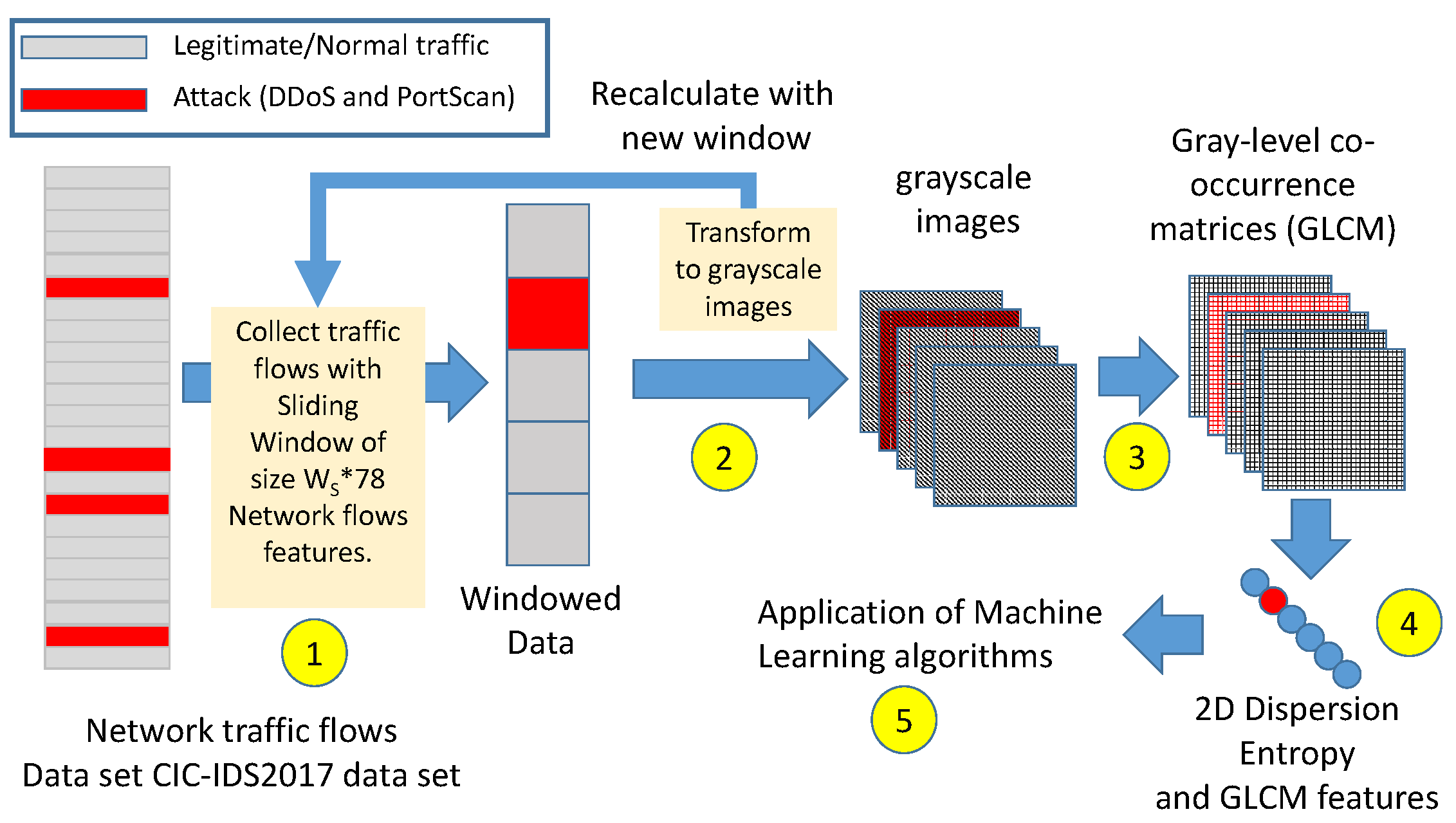
The overall workflow of the proposed approach is shown in Figure 1 where the main phases are identified with numbers. The phases are described in the following bullet list:
1.
The network flows for the labeled legitimate traffic are collected in a sliding window (the windows are not overlapping) of size W S using all the 78 network features present in CICIDS2017 data set (see Section 3.2). Different sizes W S of the sliding window are used in this study: W S = ( 100 , 200 , 300 , 400 , 500 ) network flows.
2.
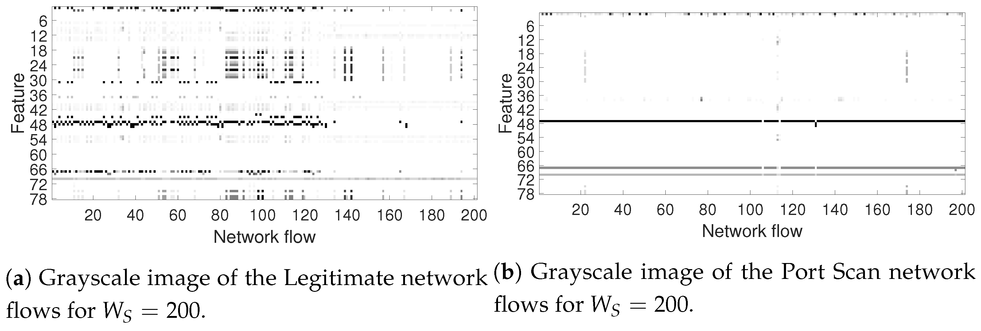
The sliding window data (of size W S 78) is converted to gray images by rescaling the values of the network flows features. The rescaling is implemented by converting the original values of the network flows in the sliding window to the range 0–256 (for each network flow feature) to obtain 256 levels of gray. A linear conversion is used. Examples of the resulting gray images for the Legitimate traffic and the Port Scan traffic are shown in Figure 2, where the y-axis represents the id of the network flow feature, while the x-axis represents the flow id. The sliding window is applied in sequential order regardless of the IP origin as it was created in the public data set [5] used in this paper.
3.
The GLCM is applied to the gray images with different values of the GLCM hyparameters. See Section 3.3 for the definition of GLCM and hyperparameters. One of the important hyperparameters is the quantization factor Q F . In other words, different GLCMs are created for each of the distances and directions considered in Section 3.3 (even for different values of G D ) and for the value of the quantization factor Q F . The resulting size of the GLCM is Q F Q F .
4.
The GLCM features (e.g., contrast) are calculated. In addition, the 2DDE is also calculated on the images. The definition of the 2DDE is presented in Section 3.4.
5.
The ML algorithm is applied to the features calculated in the previous step. The description of the algorithm used in this study and the related hyperparameters are described in the Section 3.5.
Finally, the hyperparameters of the GLCM and of the ML algorithm are tuned using the Error Rate (ER) as evaluation metric. The definition of ER and the other evaluation metrics are provided in Section 3.6.

3.2. Materials

To evaluate the proposed approach, the publicly available CICIDS2017 data set described in [5] is used. This data set was used because it is relatively recent in comparison to older data set like the KDD-99 data set, whose limitations are known and discussed in [14,21]. These limitations have prompted the research community to generate even simulated data sets like the ones proposed in [22]. The CICIDS2017 data set is based on a real network where intrusion attacks have been implemented. Then, it satisfies one of the requirements for data sets identified in [21]. As described in [5], the test bed to implement the attacks was divided into two completely separated networks: a Victim-Network and the Attack-Network. In the Victim-Network, the creators of the CICIDS2017 data set have included routers, firewalls, switches, along with the different versions of the common three operating systems: Windows, Linux and Macintosh. The Attack-Network is implemented by one router, one switch and four PCs, which have the Kali and Windows 8.1 operating systems. The Victim-Network consists three servers, one firewall, two switches and ten PCs interconnected by a domain controller (DC) and active directory. The dataset contains normal traffic (i.e., legitimate traffic with no attacks) and traffic with the most up-to-date common attacks for five days. We selected two types of attacks in this study: the DDoS attack and the PortScan attack. These attacks are chosen because they are quite representative of intrusion attacks and because they have the largest number of samples in the CICIDS2017 data set. Both attacks were generated on the last day of the data set. The DDoS traffic in this dataset was generated with a tool to flood UDP and TCP requests to simulate network layer DDoS attacks, and HTTP requests to simulate application-layer DDoS attacks. The Portscan attack was executed from all the Windows machines by the main switches. The dataset is completely labeled and includes 78 network traffic features, which were extracted using the CICFlowMeter software package described in [5]. Note that the CICflowmeter outputs 84 features including the label (see [23] for a description of all the features), but we removed features 1 (Flow Id), 2 (Source IP), 3 (Source Port), 4 (Destination IP), 5 (Destination Port) thus obtaining the 78 features used in this paper, since the last field is used as the label.
Two separate data sets are created from the original CICIDS2017 data set: one data set containing only the legitimate traffic and the Distributed Denial of Service (DDoS) network flows and another data set containing only the legitimate traffic and the Port Scan network flows. The two data sets were created by selecting from the whole data set only the network flows labelled as legitimate traffic and the specific attack: DDoS or PortScan. All the network flows from the other attacks were removed from the other data set.
Table 1 shows the number of legitimate/benign traffic samples and the attack samples for the DDoS and the PortScan attacks.
As described in Section 3.5 later in this paper, the data set is subdivided in folds, which contain exclusive portions of the data set containing both legitimate traffic and traffic related to the intrusion attack. In this study, a number of folds equal to 3 was selected to ensure to have enough samples of the attack since the CICIDS2017 data set is unbalanced like many other intrusion data sets: the number of traffic samples related to the intrusion are usually much less than the legitimate traffic ones. The application of the approach proposed in this paper is applied separately to each fold and then the values are averaged. The optimization step is also performed on averaging the results from all the folds. This technique of subdividing the data set is one of the guidelines for the application of machine learning to intrusion detection problem as suggested in [21]. It is important to point out that, in our study, we use all the 78 network flow features of the data set and we do not perform a feature selection on the network flow features as other papers have attempted [5,24]. The reason is that feature selection is performed on the GLCM features instead and we wanted to conduct the analysis on the widest set of information from the initial data set. We want to limit the degrees of freedom in the problem by not performing a feature selection on the network flows features. This is a similar approach to other papers where all the 78 Network flows features are used [25]. Future developments may investigate the selection of specific network flow features even if this task can be quite time consuming with this approach.

3.3. Gray Level Co-Occurrence Matrices

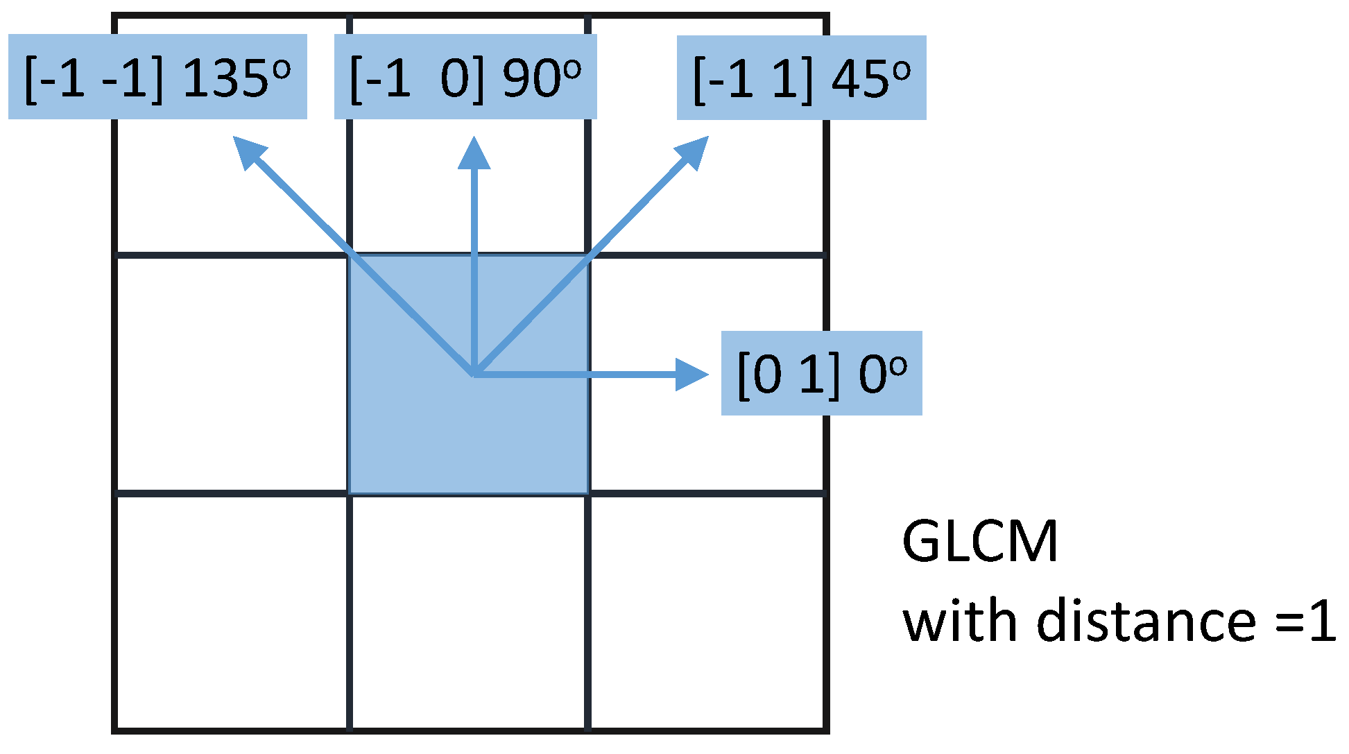
The GLCM is a statistical method for examining texture that considers the spatial relationship of pixels. The GLCM functions characterize the texture of an image by calculating how often pairs of pixel with specific values and in a specified spatial relationship occur in an image, creating a GLCM. In this context, the network flows features are used to create a grayscale image (256 levels of gray) X of size W S (where W S is the size of the sliding window) for N F (where N F is equal to the number of features or 78). Then, the GLCM is created on this grayscale image by calculating how often a pixel with the intensity (gray-level) value i occurs in a specific spatial relationship to a pixel with the value j. Each element (i,j) in the resultant GLCM is simply the sum of the number of times that the pixel with value i occurred in the specified spatial relationship to a pixel with value j in the input image. The GLCM is characterized by a number of hyperparameters in its definition: the most important is the quantization factor Q F or the number of levels. From the original 256 gray levels of the source image, the GLCM introduces a new number of gray levels, specified as an integer: the Q F . This parameter is quite important because the number of gray-levels determines the size of the resulting GLCM. This means that regardless of the size ( W S N F ) of the input grayscale image, the resulting GLCM image has size Q F Q F . The trade-off is that a larger Q F may increase the granularity of the features on which the ML is applied, thus potentially increasing the detection accuracy. On the other side of the coin, a larger GLCM (and greater values of Q F ) increases the time to calculate the GLCM features and 2D Dispersion Entropy (2DDE). Then the value of Q F must be optimized. Another hyperparameter is the distance between a pixel of interest and its neighbor. It is possible to define not only the absolute distance among pixels but also the angle as shown in Figure 3. In the rest of this paper, the absolute distance is named G D and each distance and angle is defined by a 2-tuple (e.g., [0 G D ]).
A third parameter (Symmetric or Not Symmetric) is the order of values which can be counted only once or twice. When the hyperparameter is set to Symmetric the GLCM is calculated by counting the pairings twice. When the hyperparameter is set to Not Symmetric the GLCM is calculated by counting the pairings only once.
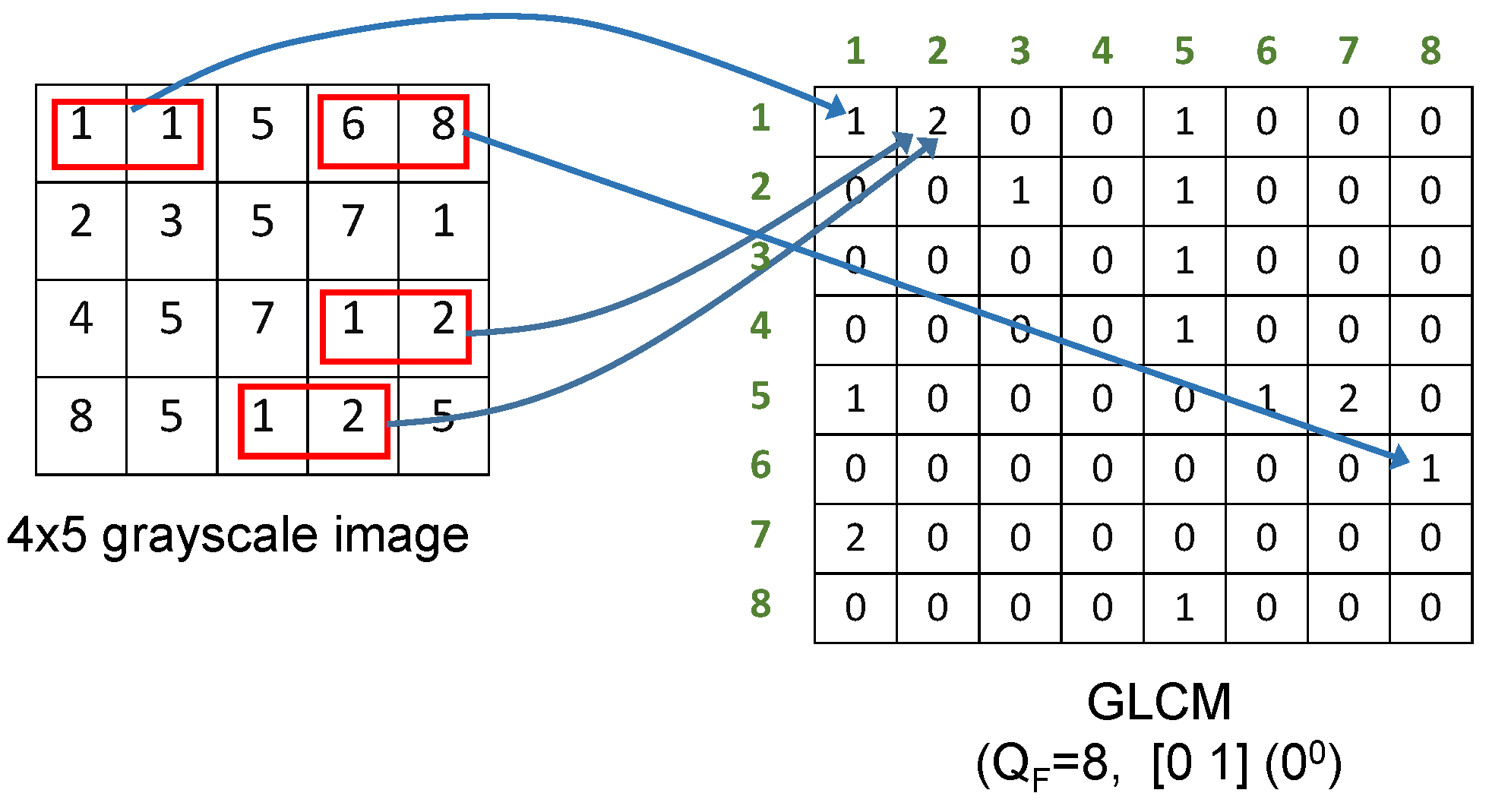
An example of the calculation of the GLCM applied to a grayscale image of size 4 5 is provided in Figure 4 where Q F = 8 and the distance/angle 2-tuple is set to [0 1].
In the original GLCM definition, it is possible to calculate the GLCM along all the possible directions, but an evaluation of the data set by the authors in this specific IDS context has shown that the additional directions not described in Figure 3 are duplications of the directions already identified and they would add unneeded computing efforts as they would grow the number of features on which the ML has to be applied. A quantitative confirmation that the angles shown in Figure 3 have an higher detection performance than using all the angles of the GLCM is provided in Section 4. Then, in the rest of this paper, we will use the 2-tuples [0 G D ], [− G D 0], [− G D G D ], [− G D G D ].
As described in the Introduction Section 1, the idea to use GLCM in the context of IDS is that the sequential structure of the network flows in case of an intrusion is altered in comparison to the legitimate traffic. Since the GLCM is created by calculating how often pairs of pixels with a specific value and offset occur in the image, the underlying idea of the approach is that numbers of pairs of pixels will be altered when an attack is implemented. The challenge is that it is not known a priori how the choice of values of the hyperparameters influences the detection accuracy of the intrusion attack, since this information depends on the context (e.g., the topology of the network, the type of traffic and the type of attack). Then, an optimization process has to be performed, which is described in detail in Section 4.1.

3.4. Two Dimensional Dispersion Entropy

Two dimensional dispersion entropy (2DDE) was introduced by Azami and others in [4] where it is described in detail. Here, we provide a brief description of the 2DDE measure with reference to the IDS problem.
2DDE is an extension of the one dimension dispersion entropy, which has demonstrated its superior performance in many problems [26]. The original definition of 2DDE is applied to an image of size w h , but in this study, the GLCM is the image on which the 2DDE is to be calculated and its size is equal to Q F Q F , then the equations and definitions from [4] are modified accordingly.
In a first step, each value in the image U (i.e., the GLCM image in this case) is mapped to classes with integer indices from 1 to c (which is one of the hyperparameters in the definition of 2DDE). To this aim, there are a number of linear and nonlinear mapping approaches, which can be used in the dispersion entropy based methods. The simplest and fastest algorithm is the linear mapping. However, when maximum or minimum values are noticeably larger or smaller than the mean/median value of the image (as in this case where anomalies significantly greater than the average must be detected), it is preferable to use a sigmoid function as defined in [4], where the normal cumulative distribution function (NCDF) is used to map the image into the classes, as this function naturally raises in a sigmoidal shape. The NCDF maps the initial image U (i.e., the GLCM of the window traffic) to Y with values from 0 to 1 as in the following equation:
y i , j = 1 σ 2 π x i , j e ( t μ ) 2 2 σ 2 d t
where μ and σ are the average and standard deviation of U.
The concept of Dispersion Entropy (even the one in one dimension) is related to the patterns of the embedding dimension m (another hyperparameter in the definition of 2DDE). The dispersion patterns are created in the following way.
First, a new matrix z z k , l m , c is created from y i , j using the following equations (this is the adaption of Equation (2) from [4] taking in consideration that w and h from (2) are equal to Q F in this case):
z k , l c = r o u n d ( c × y i , j + 0.5 )
where z k , l c shows the ( i , j ) th of the classified image and rounding involves either increasing or decreasing a number to the next digit.
Second, z k , l m , c are made with the embedding dimension vector according to the following equation.
z k , l m , c = z k , l c , z k , l + 1 c , z k , l + 2 c , , z k , l + ( m Q F 1 ) c , z k + 1 , l c , z k + 1 , l + 1 c , z k + 1 , l + 2 c , , z k + 1 , l + ( m Q F 1 ) c , , z k + ( m Q F 1 ) , l c , z k + ( m Q F 1 ) , l + 1 c , z k + ( m Q F 1 ) , l + 2 c , , z k + ( m Q F 1 ) , l + ( m Q F 1 ) c
where k, l = 1, 2, ..., Q F ( m Q F −1).
Third, each term of the matrix z k , l m , c is mapped to a dispersion pattern π v j on which the final entropy measure 2DDE is calculated in the following way.
Fourth, for each c m Q F x m Q F potential dispersion pattern π v 0 , v 1 , , v ( m Q F 1 ) , the relative frequency π v 0 , v 1 , , v ( m Q F 1 ) in the image Y is calculated.
Finally, the Shannon entropy is calculated on the dispersion pattern π v 0 , v 1 , , v ( m Q F 1 ) to provide the 2DDE according to the following equation:
2 D D E ( m , c ) = π = 1 c m Q F × m Q F p ( π v 0 , v 1 , , v ( m Q F 1 ) × ( m Q F 1 ) ) × l n p π v 0 , v 1 , , v ( m Q F 1 ) × ( m Q F 1 )
As in one dimension dispersion entropy, the value of the parameters m and c should be tuned to achieve an optimal performance (in this case, the detection of the attack). On the other side, the parameters m and c are bound [4] by the size of the time series on which 2DDE has to operate. As described in [27] even for the one dimension dispersion entropy, to work with reliable statistics when calculating dispersion entropy, it is suggested that the number of potential dispersion patterns c m is smaller than the length of the signal. In the two dimensional case, the rule reported in [4] and adapted for this case where the GLCM is square of size Q F Q F , is that ( c m Q F ) 2 < ( Q F m Q F 1 ) 2 , which limits the space of the values of m and c to few values as the range of Q F . Considering that the range of Q F spans from 12 to 48 in this study, the combinations of c = 2, m = 3 and c = 3, m = 2 are chosen. It must also be taken in consideration that higher values of m increase the computing time, which is not desirable for a large data set like the one used in this study.
As pointed out in the Introduction, the rational for using 2DDE in this study is that 2DDE allows to analyze irregularity of images on the basis of the frequency of the dispersion patterns in the image [4], which can provide more information than the classical Shannon Entropy. Since an intrusion attack usually disrupts the regularity of the structure of legitimate traffic, the application of 2DDE can provide a significant discriminating power for the detection of the attack.

3.5. Machine Learning Algorithms

The following machine learning algorithms were used in the study: the Support Vector Machine, the Decision Tree and Naive Bayes algorithm. These algorithms were chosen because they have already been used in literature [5,24] on the same problem because of their accuracy and cost effectiveness. These three algorithms are also chosen because each of them belongs to a specific category of machine learning algorithms and they are useful to provide a comparison on the relevance of the algorithm to the IDS problem. We would like anyway to remark that the goal of the paper is the investigation on the discriminating power of the approach based on GLCM and 2DDE rather than the choice of a specific machine learning algorithm. In other words, they are used rather to understand the relevance of the different features for the detection of benign and malicious activity, which can eventually serve as the basis for a non-machine-learning detector [14].
Support Vector Machine (SVM), is a supervised learning model which classifies data by creating a hyperplane or set of hyperplanes in a high dimensional space, to distinguish the samples belonging to different classes (two classes in this problem). Various kernels have been tried and the one providing the best performance was the Radial Basis Function (RBF) kernel, where the values of the scaling factor γ must be optimized together with the parameter C [28].
The Decision Tree algorithm is a predictive modeling approach where a decision tree (as a predictive model) analyzes the observations about an item (represented in the branches) to reach conclusions about the item’s target value (represented in the leaves). In this case we use classification trees where leaves represent class labels and branches represent conjunctions of features that lead to those class labels. The hyperparameter chosen for optimization is the maximum number of branches at each split named N B in the rest of this paper. It was chosen the option that the algorithm trains the classification tree learners without pruning them. The optimal values for the three machine learning algorithms are presented in Section 4.
The Naive Bayes (NB) machine learning algorithm is a probabilistic classifier, which is based on applying Bayes’ theorem with strong (naïve) independence assumptions between the features [29]. In the NB algorithm, models assign class labels to problem instances, represented as vectors of feature values, where the class labels are drawn from some finite set. In many practical applications like IDS, the parameter estimation for the NB models uses the method of maximum likelihood; which means that the NB classifier can be applied even without accepting Bayesian probability.
As discussed before, for the application of all machine learning algorithms, a 3-fold approach (i.e., K-fold approach with K = 3) was used for classification, where 1/3 of the dataset was used for test, and 2/3 was used for training and validation. The portions of the data set in each fold are exclusive among themselves. The value of 3 was used to subdivide the data set in portions large enough to ensure that a meaningful set of data related to the intrusion is present in the input data to the classifiers. Then, the attack data was also split in 3 as part of the overall 3-fold approach. Since intrusion data sets are usually heavily unbalanced (legitimate traffic is much larger than traffic related to the intrusion), there is the risk that high values of K produce folds with a limited number of samples related to the attack. To further generalize the application of the approach, the overall classification process was then repeated 10 times, each time with different training and test sets. The final results were averaged.
As it is seen in the Section 4, the Decision Tree algorithm provides the optimal detection accuracy for this problem.

3.6. Detection Metrics

This subsection describes the metrics used to evaluate the performance of the approach proposed in this paper and the alternative approaches used in literature.
The main metric is the Error Rate (ER), which is 1-Accuracy and it is defined as:
ER = 1 TP + TN ( TP + FP + FN + TN )
where TP is the number of True Positives, TN is the number of True Negatives, FP is the number of False Positives and FN is the number of False Negatives.
To complement the accuracy metric, the True Positive Rate (TPR) and the False Positive Rate (FPR) are used, which are defined in the following equations:
TPR = TP ( TP + FN )
FPR = FP ( FP + TN )
Another method to evaluate the performance of the approach proposed in this paper, is the Receiver Operative Characteristics (ROC) curve which is created by plotting the True Positive Rate (TPR) against the False Positive Rate (FPR) at various threshold settings. A metric based on the ROC curve is the Equal Error Rate (EER), which is the point on the ROC curve that corresponds to have an equal probability of miss-classifying a positive or negative sample.

3.7. Features and Hyperparameters

As specified before, the proposed approach is based on a number of hyperparameters, which are summarized in the following bullet list with the related trade-offs:
  • W S = the size of the sliding window. The trade-off is that a small value of W S does not provide an image large enough for the application of GLCM while a large value of W S limits the number of samples for the application of ML.
  • Q F = Quantization factor in GLCM. A value too small may not provide enough granularity for an effective detection of the threat while a value, which is too large increases significantly the computing time.
  • GLCM distance and angle parameter in GLCM definition. There are no trade-offs but the optimal value must be selected.
  • GLCM symmetry. If the GLCM is applied with symmetry or asymmetry. There are no trade-offs but the optimal value must be selected.
  • c and m in the 2DDE definition. c and m are bound by the value of Q F as specified in [4].
  • hyperparameters in the ML algorithm. For example, the maximum number of branches at each split in the Decision Tree algorithm.
Beyond the hyperparameters identified above, a number of features were proposed by Haralick in its seminal paper on the design of GLCM and the related feature [30,31], but not all the Haralick features are applicable to this context, either because they are computing intensive, because they are unstable for small images or because they are not relevant for the context. In addition, the use of all the Haralick Features in combination for the hyperparameters identified above would generate a search space which would be too large for the optimization process. After a preliminary assessment of the Haralick features, the following set of features were used for this study and they are listed in Table 2. The approach presented in this paper was to combine a pre-selected set of Haralick features in addition to 2DDE with the GLCM symmetry and GLCM distance and angle parameter hyperparameters. The other Haralick features described in [31] were not used because their detection performance using ER was suboptimal in comparison to the features identified in Table 2: Difference Variance, Difference Entropy, Info Measure of Correlation, Maximum Correlation Coefficient. Note that in Table 2, Energy indicates the angular second moment and Homogeneity is the inverse difference moment on the basis of the terms described in [31].
As it is shown in Table 2 the GLCM is calculated on the gray image (created from the sliding window) for different values of the angle for a specific value of the distance G D . Then, the related features for each specific GLCM are calculated. For example, one GLCM is calculated for the angle [0 G D ] while another GLCM is calculated for the angle [− G D G D ].
The optimal set of features are selected using the forward sequential feature selection. In the forward sequential search algorithm, optimal features are added to a candidate subset while evaluating the criterion. Since an exhaustive comparison of the criterion value at all subsets of the 64 features from Table 2 (repeated for all the values of the hyperparameters) is typically infeasible, the forward sequential search moves only in the direction of growing from an initial feature (the one with the lowest ER when all the features are considered). The best ten features are used to calculate the final metrics of evaluation: ER, FPR, FNR. The number of ten has been adopted because it was the optimal value between the need to limit the number of features for the application of ML and the increase of detection accuracy (beyond ten features, the improvement in detection accuracy was minimal).
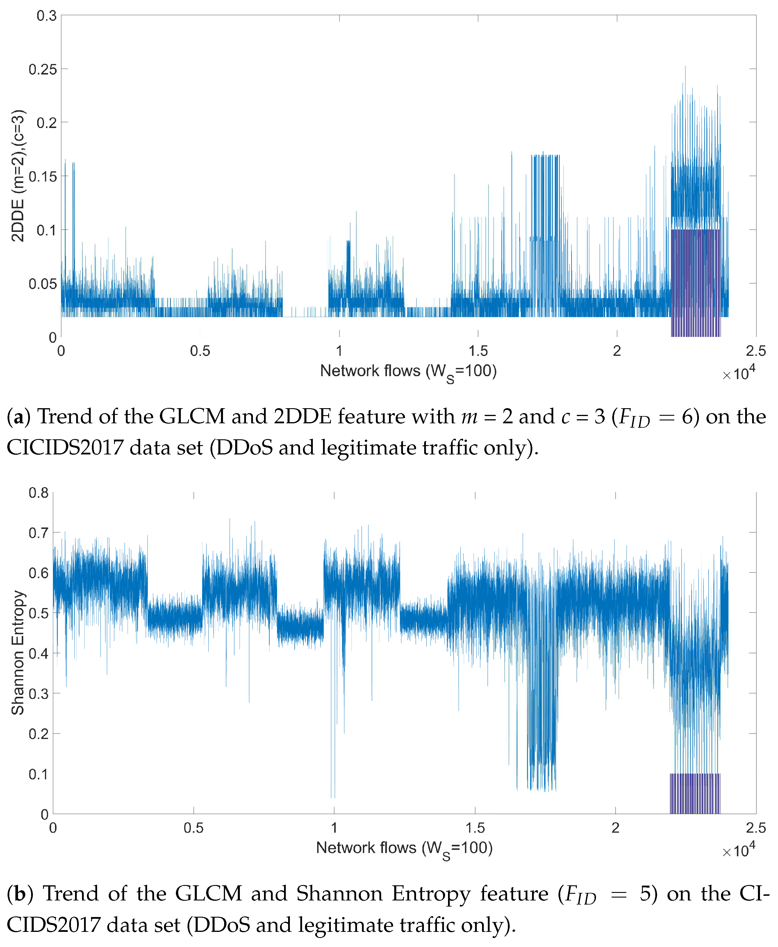
Apart from the application of the ML algorithms, the difference of the discriminating power of 2DDE in comparison to the other features to detect an attack can be visualized by the trends of the features in comparison to the network flows features. Figure 5a,b show respectively the trend of GLCM-2DDE and GLCM-Entropy (i.e., Shannon Entropy) for the Port Scan attack. The blue plot shows the trend of the specific feature while the bar graph (purple bars superimposed on the plot) identifies the windows where the attack is implemented and labelled. It can be seen in Figure 5a that the values of GLCM-2DDE (called simply 2DDE in the rest of this paper) are notably higher in correspondence to the Port Scan attack than the normal legitimate traffic. This difference is less evident for the GLCM-Entropy feature. These differences in values are the reason why the performance of GLCM-2DDE is higher than the GLCM-Entropy when ML is applied.
We highlight that Figure 5 and the previous paragraph are only used for informational purposes to provide to the reader with a visual recognition of the difference of the trends in the data set once two different entropy measures are applied to the network flows data. Figure 5 is not used to select features for the classification phase because the SFS is used for this purpose as described in Section 4.

4. Results

4.1. Optimization

This sub-section provides the results on the optimization of the hyperparameters described in the previous sections.
A grid approach was used to determine the optimum values of the hyperparameters. While, other methods (e.g., gradient, meta-heuristics algorithms) could be more efficient, it should be considered that the ranges of values for each hyperparameter are quite limited. In addition, the intention is to show in an explicit way the impact of each hyperparameter for the detection performance. The metric is used to determine the optimal values of the hyperparameters.
The summary of the hyperparameters used in this study, the optimal values and the range of the hyperparameters are shown in Table 3. In the rest of this sub-section and related figures, we show how a specific hyperparameter impacts the detection accuracy of the threat both for DDoS attack and Port Scan attack. For each presented result, the other hyperparameters are set to the values identified in Table 3. The Decision Trees (DT) ML algorithm was used to generate the results provided in this sub-section. As shown in Section 4.3 the DT algorithm has a higher detection performance than the SVM and Naive Bayes algorithms.
The following figures describe the results for the evaluation of the proposed approach for different values of the hyperparameters and for the different features used in the study. In most cases, the evaluation of a single hyperparameter is provided while the other hyperparameters are set to the values described in Table 3 unless otherwise noted.
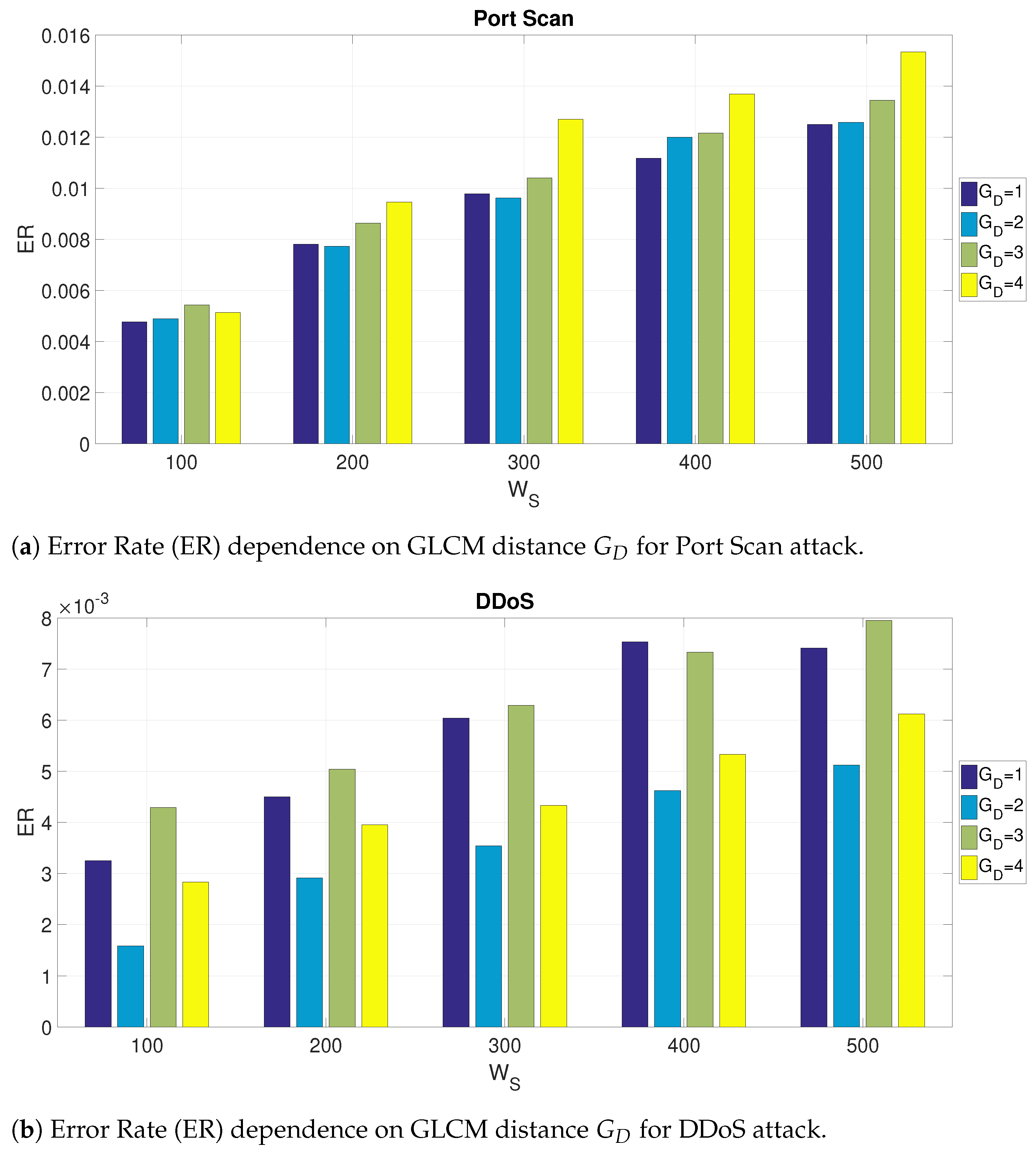
Figure 6a,b show respectively for the Port Scan and the DDoS attacks, the impact of the GLCM distance G D for different values of the window size W S . These results are obtained using all the 64 features identified in Table 2. It can be noted that the optimal value of W S is 100 network flows, as the ER increases with larger values of W S . This may due to the reasons that the difference between legitimate traffic and the traffic related to the attack are more evident when the W S is relatively small. On the other side, W S = 100 is the lower limit of W S to allow the GLCM to operate on a grayscale picture large enough to obtain meaningful values. Figure 6a shows that a value of G D = 1 is optimal to detect the Port Scan attack, while Figure 6a shows that a value of G D = 2 is optimal for the DDoS attack. These results seem to indicate that there is no need to use values of G D larger than 2, which would also be more computing intensive.
Then, the impact of the quantization factor Q F was evaluated. As described before, the quantization factor in the GLCM definition is an important factor in the application of GLCM. A large value of Q F provides an higher granularity which can be beneficial in the application of the ML algorithm for the detection of the threat. On the other side, a large value of Q F is more computing expensive for the calculation of the GLCM features and 2DDE as the resulting GLCM matrix are larger (the GLCM size is Q F Q F ). This is an important trade-off, which was investigated for each specific feature and for each attack.
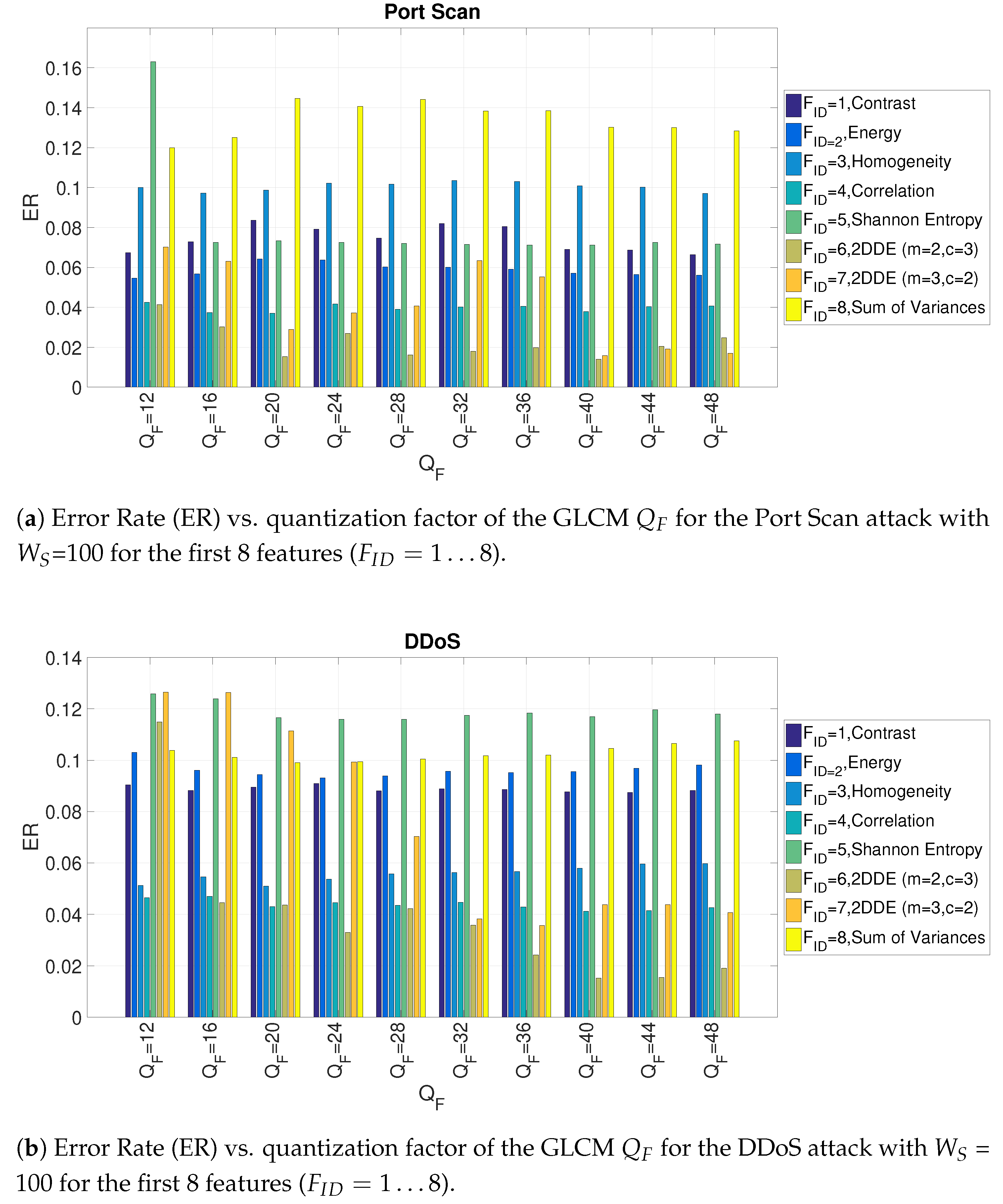
Figure 7a,b shows the impact of the Q F parameter on the detection accuracy respectively for the Port Scan and the DDoS attack for the first 8 features (only the first 8 features are provided in these figures for reasons of space, but subsequent figures will consider all features). The value of W S is set to 100 since the previous Figure 6 has shown that W S = 100 is the optimal value for attack detection. Figure 7a,b provide two important results: the first is that they identify the optimal value of the Q F parameter ( Q F = 40 for the Port Scan attack and Q F = 44 for the DDoS attack). The second is that they show that the 2DDE features have a better performance than the other features. This result justifies the assumption done in this paper for the application of 2DDE to the problem of IDS.
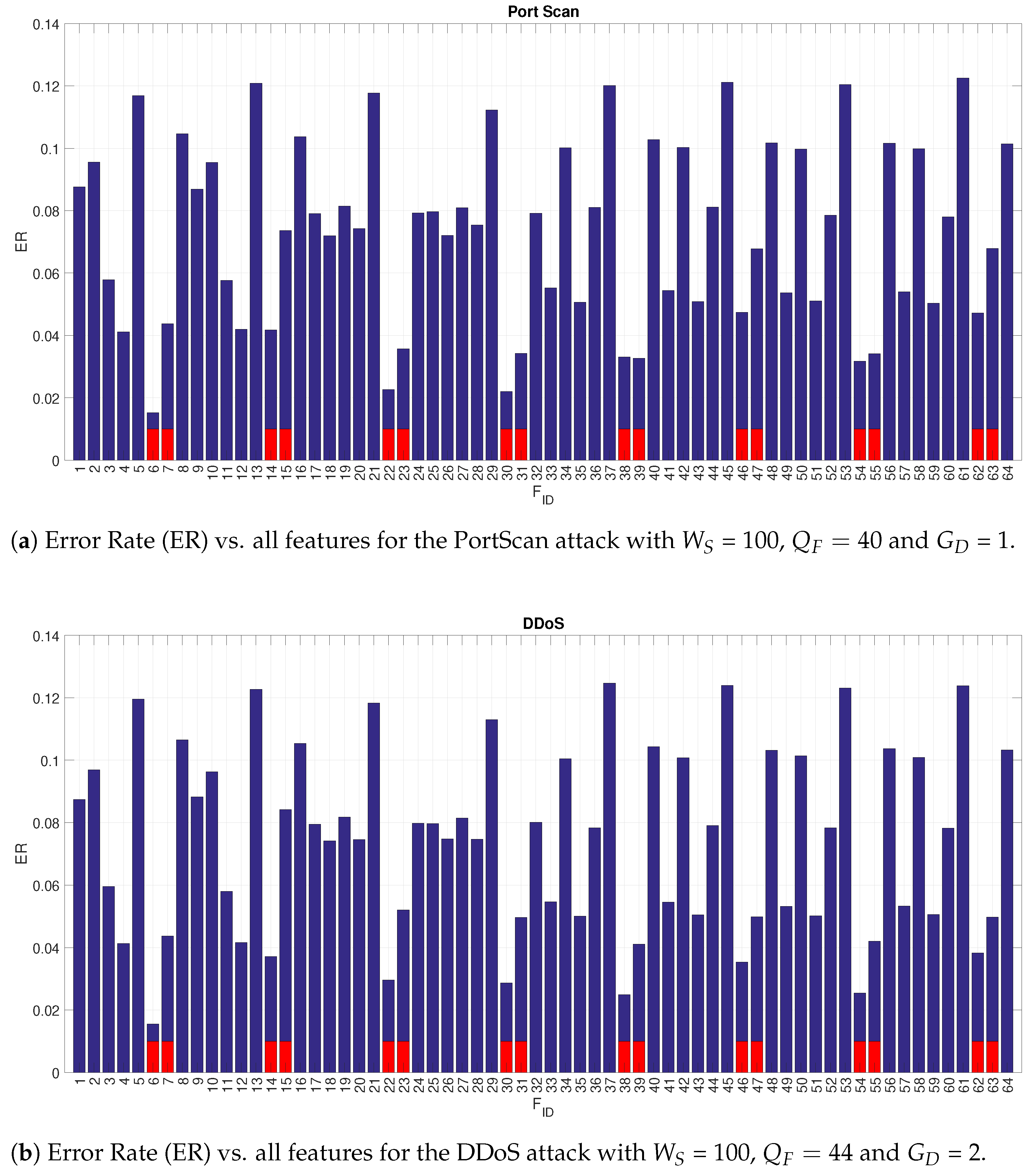
Figure 7 shows only the first 8 features. Then, a more extensive analysis of the detection performance of each of the 64 features was carried on by setting the optimal value of the other hyperparameters ( G D , Q F and W S ). The results are shown in Figure 8a,b where the ER is reported for each feature identified with the F I D identifier. To better visualize the features related to 2DDE a red bar is used in the Figures. Figure 8a,b show that the 2DDE is able to obtain a consistent high detection accuracy in comparison to the other features for all the 64 features. In particular, for both attacks, the values of m = 2 and c = 3 in the 2DDE definition provides a better performance than the values of m = 3 and c = 2 in the 2DDE definition. This result shows the higher detection performance of 2DDE in comparison to the other features (e.g., Shannon entropy or variance). The results shown in these figures also give an indication on the GLCM angle, which is most performing. In general, the GLCM distance and angle defined by the 2-tuple [0 G D ] (which corresponds to F I D = 1 8 ) provides better results (in terms of detection accuracy) than the other 2-tuples.
The importance of 2DDE in comparison to other features for the IDS problem is also visible, once SFS is applied to select the optimal set of features on the basis of the value of hyperparameters already set. The results of the application of SFS is presented in Table 4, where the 10 best features are shown respectively for the DDoS and the Port Scan attack. In Table 4, the 2DDE features are highlighted in red. It can be seen that the 2DDE features are substantially present among the 10 best features, which shows the the application of 2DDE to this specific problem is an important element to achieve an higher detection accuracy of the attack.

4.2. Optimized Results

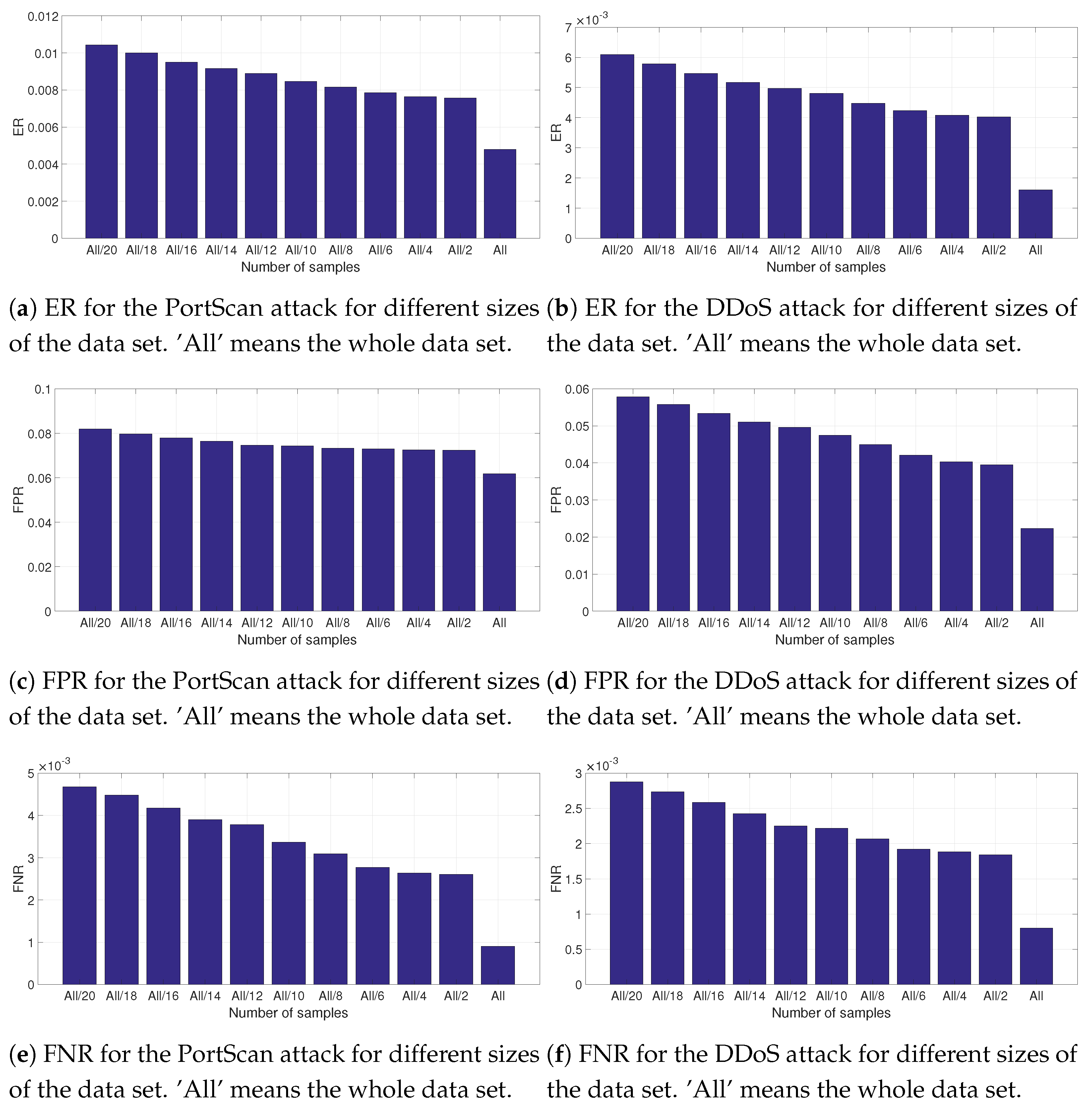
On the basis of the best features described in Table 4 and the optimal values of the hyper-parameters defined in Table 3, the ER, FPR and FNR have been calculated using the Decision Tree algorithm. It was also evaluated the impact of the size of the data set. From the whole data set, a partitions of the whole data set have been selected and the ER, FPR and FNR have been calculated. The results are presented in Figure 9 and related subfigures where ’All’ means the whole data set and ’All/x’ is a partition by the factor x. The size of ’All’ can be calculated from the values presented in Table 1. The partition is created by extracting randonmly ’All/x’ elements from the whole data set. To mitigate the risk of bias, the selection of the partition and the calculation of the results is repeated 100 times and the results are averaged.
Both for the PortScan and the DDoS attacks, it can be seen that the performance of the detection of the attack is lower for smaller partitions of the data set because it is more difficult for the algorithm to discriminate the legitimate traffic from the traffic related to the attack. This trend is coherent for all the three metrics (ER, FPR and FNR) and the two attacks.
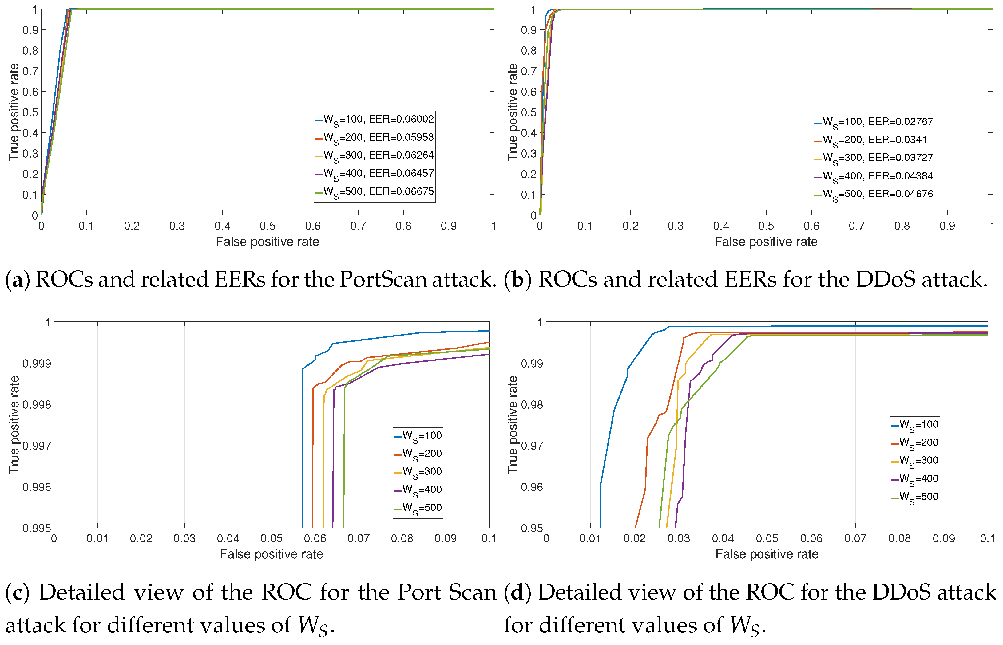
To complete the previous results, the ROCs for the DDoS and the PortScan attacks are presented respectively in Figure 10a,b. Since the FPR is relatively limited (because the data set is quite unbalanced), a more detailed figure of the same ROCs (i.e., zoom of the previous figures) is presented in Figure 10a,b respectively for the DDoS and the PortScan attacks. The values of the E E R for each value of W S are also reported. The results from the ROCs confirm the previous result that the optimal value of the window size is W S = 100 because an increase of W S produces slightly worst results in terms of ROCs and EER. It can also been seen that the detection of the PortScan attack is slightly worse than the DDoS attack. This may be due to the reason that PortScan attacks are more difficult to distinguish from legitimate traffic than the DDoS attacks when the entropy measures are applied (especially in the CIC-IDS2017 data set). The structure of the sequences of network flows features in the DDoS attacks can be quite different from legitimate traffic (e.g., since a flooding of messages is implemented) while the PortScan attack traffic may resemble legitimate traffic. The weakness of the proposed approach in achieving an optimal FPR is also discussed in the comparison with the literature results in Section 4.3. We note that the proposed approach manages to achieve a very competitive FNR instead.

4.3. Comparison with Other Studies

On the basis of the optimization results obtained in the previous Section 4.1, we have calculated the values of ER, FPR and FNR for the Port Scan and the DDoS attack and we compared these results with the results in literature on the same CICIDS2017 data set. The comparison is indicative because each study may have modified the initial data set in different ways: a subset of the initial 78 features may be used or the data pertaining only to specific attacks has been used. We must also consider that the CICIDS2017 data set is relatively recent and not all the studies using it focused on a specific attack as it was done in this study. The results are presented in Table 5 where the first three columns identify the value of ER,FPR and FNR. The fourth column provides relevant notes (e.g., the specific adopted algorithm). The fifth column identifies the specific attack (i.e., DDoS or Port Scan) and the related study where the results were produced. Table 5 does also provides the comparison of the machine learning algorithms: SVM algorithm, Naive Bayes algorithm and Decision Tree.
The results show that the proposed approach is competitive against other approaches proposed in literature. For example, in the case of the DDoS attack, the obtained ER (0.0016) is smaller than the ER obtained by most of the other results with the exception of the study [7] where it has the same value or the study [6] where the obtained ER is slightly lower than the result obtained in this study (0.0015 rather than 0.0016). It has to be noted that both [6,7] use sophisticated DL algorithms which are more computing demanding than the approach proposed in this paper. In addition, it is noted that the approach proposed in this paper is able to obtain a value of False Negative Rate (FNR) for the DDoS attack (i.e., 0.00079), which is considerable lower than the result obtained by all other approaches. On the other side, the FPR is worse than the value obtained by the other studies. Then, this approach is particularly strong on the FNR performance but it is weaker on the FPR. A potential reason why FNR is so low in comparison to literature is due to the sliding window approach where the presence of only a single network flow labelled as an attack in the data set is magnified to the size of the sliding window. The improvement of the FPR is one of the actions for future developments and investigations on this approach.
The results obtained with the DDoS attack are confirmed by the results obtained by the PortScan attack. The obtained FNR is better than the results obtained in literature while the ER is also smaller than the results presented in other studies. In particular, our approach achieves a similar ER to the results in [9], which uses a DL approach (i.e., LSTM). On the other side, the FPR obtained with this approach is higher than the results obtained in literature. Another result shown in Table 5 is that the Decision Tree algorithm has a better detection performance than the SVM and Naive Bayes algorithms. This result is consistent with [5] where the DT provided the optimal detection accuracy.
An evaluation of the use of all the GLCM angles was also implemented to validate the adoption of only a limited set of GLCM angles as described in Section 3.3. The results are provided in Table 6 using the Decision Tree algorithm. The results in Table 6 show that a subset of the GLCM angles (as selected in this study) provides a better performance than using all angles since the ERs for the subset are smaller than the ERs for all the GLCM angles. The results are consistent for different values of W S and for both attacks of PortScan and DDoS.
4.4. Computing Times

In the following Table 7, we report the computing time of the proposed approach with the application of ML directly on the data set in a similar way to what was done in the paper [5]. The approach proposed in this paper implements a dimensionality reduction and the computing time to execute the machine learning algorithm on the reduced set is minimal. On the other side, the time requested to calculate the GLCM is significant (34 s in average for the DDoS attack and 31 s in average for the PorScan attack) as shown in Table 7. The average time needed to calculate the 2DDE entropy measure is also relatively high (63 s for the DDoS attack and 83 s for the PortScan attack). These calculated times are based on W S = 100 since this was the window size with the minimum ER and the optimal selection of features presented in Table 4. In this study, it was used a laptop with Intel i7 85550U CPU running at 1.8 GHz with 16 GBytes of RAM and no GPU.

5. Conclusions

This study proposes a novel approach for IDS based on anomaly detection which is based on the transformation of the network flows metrics into grayscale images. Then, the Gray-Level Co-occurrence Matrices (GLCM) are calculated on the grayscale images and features are calculated on the GLCM. Beyond the application of well known GLCM Haralick features (i.e., contract, homogeneity, entropy), this paper proposes the novel application of 2D Dispersion Entropy (2DDE) recently proposed in literature. The results show that the application of 2DDE to GLCM significantly enhances the detection accuracy of the proposed IDS. The approach is applied to the recently published CICIDS2017 data set for two specific attacks: DDoS and Port Scan. The results of this approach are compared with the results obtained by other studies on the same CICIDS2017 data set obtaining an Error Rate (ER) which is higher or comparable with the results obtained with more sophisticated approach based on Deep Learning, which requires considerable more computing resources than our proposed approach. In addition, the False Negative Rate (FNR) obtained with our approach is significantly better than all the other results obtained in literature. On the other side, the False Positive Rate (FPR) is slightly worse than the results obtained in literature. This may due to the possibility that the transformation of the network flows features to gray level images and then GLCM-base features has the tendency to lose the specific characteristics of the attack related traffic in comparison to the normal traffic.
Future developments will try to improve the FPR by adopting improvements of the proposed approach in different directions. One direction would be to use Fuzzy Gray-Level Co-occurrence Matrices since it has demonstrated a superior performance in some applications, but it has not been used in IDS problems. Another direction would be the application of non linear GLCM where the quantization factor is calculated in a non linear way. The significant number of hyperparameters to tune in the approach (both in the GLCM definition and 2D dispersion entropy definition) is also a challenge to mitigate for a practical deployment of this approach. One possibility to resolve the challenge would be to investigate the application of meta-heuristics algorithms (e.g., particle swarm optimization) to automatically tune the hyperparameters. Another possibility would be to investigate the hyperparameters optimization in other data sets to generalize the selection of the optimal values. Finally, the combination of GLCM together with Deep Learning algorithms will also be considered. For example, Convolutional Neural Networks (CNN) could be applied to the GLCM representations rather than the initial gray-scale images derived directly from the network flows statistics.

Author Contributions

Conceptualization, G.B., J.L.H.R. and I.A.; methodology, G.B.; writing G.B., J.L.H.R., I.A.; funding acquisition, G.B., J.L.H.R. All authors have read and agreed to the published version of the manuscript.

Funding

This work has been partially supported by the European Commission through project SerIoT funded by the European Union H2020 Programme under Grant Agreement No. 780139. The opinions expressed in this paper are those of the authors and do not necessarily reflect the views of the European Commission.

Institutional Review Board Statement

Not applicable.

Informed Consent Statement

Not applicable.

Data Availability Statement

This study used the public data set described in [5].

Acknowledgments

We are thankful to Anne Humeau-Heurtier and the other authors of [4] to graciously provide the MATLAB code for the implementation of the 2D Dispersion Entropy.

Conflicts of Interest

The authors declare no conflict of interest.

Abbreviations

The following abbreviations are used in this manuscript:
CNNConvolutional Neural Networks
2DDE2D Dispersion Entropy
DDoSDistributed Denial of Service
DLDeep Learning
DTDecision Tree
ERError Rate
EEREqual Error Rate
FPFalse Positives
FPRFalse Positives Rate
FNFalse Negatives
FNRFalse Negatives Rate
GLCMGray-Level Co-occurrence Matrices
KOADKernel Online Anomaly Detection
NCDFNormal Cumulative Distribution Function
IDSIntrusion Detection Systems
MLMachine Learning
NCDFNormal Cumulative Distribution Function
RBFRadial Basis Function
ROCReceiver Operating Characteristics
SFSSequential Feature Selection
SVMSupport Vector Machine

References

  1. Lunt, T.F. A survey of intrusion detection techniques. Comput. Secur. 1993, 12, 405–418. [Google Scholar] [CrossRef]
  2. Liao, H.J.; Lin, C.H.R.; Lin, Y.C.; Tung, K.Y. Intrusion detection system: A comprehensive review. J. Netw. Comput. Appl. 2013, 36, 16–24. [Google Scholar] [CrossRef]
  3. Dromard, J.; Roudière, G.; Owezarski, P. Online and scalable unsupervised network anomaly detection method. IEEE Trans. Netw. Serv. Manag. 2016, 14, 34–47. [Google Scholar] [CrossRef] [Green Version]
  4. Azami, H.; da Silva, L.E.V.; Omoto, A.C.M.; Humeau-Heurtier, A. Two-dimensional dispersion entropy: An information-theoretic method for irregularity analysis of images. Signal Process. Image Commun. 2019, 75, 178–187. [Google Scholar] [CrossRef]
  5. Sharafaldin, I.; Lashkari, A.H.; Ghorbani, A.A. Toward Generating a New Intrusion Detection Dataset and Intrusion Traffic Characterization; ICISSP: Funchal, Portugal, 2018; pp. 108–116. [Google Scholar]
  6. de Souza, C.A.; Westphall, C.B.; Machado, R.B.; Sobral, J.B.M.; dos Santos Vieira, G. Hybrid approach to intrusion detection in fog-based IoT environments. Comput. Netw. 2020, 180, 107417. [Google Scholar] [CrossRef]
  7. Yu, X.; Li, T.; Hu, A. Time-series Network Anomaly Detection Based on Behaviour Characteristics. In Proceedings of the 2020 IEEE 6th International Conference on Computer and Communications (ICCC), Chengdu, China, 11–14 December 2020; pp. 568–572. [Google Scholar]
  8. Al-Sawwa, J.; Ludwig, S.A. Performance evaluation of a cost-sensitive differential evolution classifier using spark–Imbalanced binary classification. J. Comput. Sci. 2020, 40, 101065. [Google Scholar] [CrossRef]
  9. Hossain, M.D.; Ochiai, H.; Fall, D.; Kadobayashi, Y. LSTM-based Network Attack Detection: Performance Comparison by Hyper-parameter Values Tuning. In Proceedings of the 2020 7th IEEE International Conference on Cyber Security and Cloud Computing (CSCloud)/2020 6th IEEE International Conference on Edge Computing and Scalable Cloud (EdgeCom), New York, NY, USA, 1–3 August 2020; pp. 62–69. [Google Scholar]
  10. Çakmakçı, S.D.; Kemmerich, T.; Ahmed, T.; Baykal, N. Online DDoS attack detection using Mahalanobis distance and Kernel-based learning algorithm. J. Netw. Comput. Appl. 2020, 168, 102756. [Google Scholar] [CrossRef]
  11. Moustafa, N.; Hu, J.; Slay, J. A holistic review of network anomaly detection systems: A comprehensive survey. J. Netw. Comput. Appl. 2019, 128, 33–55. [Google Scholar] [CrossRef]
  12. Zarpelão, B.B.; Miani, R.S.; Kawakani, C.T.; de Alvarenga, S.C. A survey of intrusion detection in Internet of Things. J. Netw. Comput. Appl. 2017, 84, 25–37. [Google Scholar] [CrossRef]
  13. Liu, H.; Lang, B. Machine Learning and Deep Learning Methods for Intrusion Detection Systems: A Survey. Appl. Sci. 2019, 9, 4396. [Google Scholar] [CrossRef] [Green Version]
  14. Sommer, R.; Paxson, V. Outside the closed world: On using machine learning for network intrusion detection. In Proceedings of the 2010 IEEE Symposium on Security and Privacy, Berleley/Oakland, CA, USA, 16–19 May 2010; pp. 305–316. [Google Scholar]
  15. Behal, S.; Kumar, K.; Sachdeva, M. D-FACE: An anomaly based distributed approach for early detection of DDoS attacks and flash events. J. Netw. Comput. Appl. 2018, 111, 49–63. [Google Scholar] [CrossRef]
  16. Radivilova, T.; Kirichenko, L.; Alghawli, A.S. Entropy Analysis Method for Attacks Detection. In Proceedings of the 2019 IEEE International Scientific-Practical Conference Problems of Infocommunications, Science and Technology (PIC S&T), Kiev, Ukraine, 8–11 October 2019; pp. 443–446. [Google Scholar]
  17. Shah, S.B.I.; Anbar, M.; Al-Ani, A.; Al-Ani, A.K. Hybridizing entropy based mechanism with adaptive threshold algorithm to detect ra flooding attack in ipv6 networks. In Computational Science and Technology; Springer: Berlin/Heidelberg, Germany, 2019; pp. 315–323. [Google Scholar]
  18. Zhang, Y.; Chen, X.; Jin, L.; Wang, X.; Guo, D. Network intrusion detection: Based on deep hierarchical network and original flow data. IEEE Access 2019, 7, 37004–37016. [Google Scholar] [CrossRef]
  19. Lopez-Martin, M.; Carro, B.; Sanchez-Esguevillas, A.; Lloret, J. Conditional variational autoencoder for prediction and feature recovery applied to intrusion detection in iot. Sensors 2017, 17, 1967. [Google Scholar] [CrossRef] [Green Version]
  20. Zhou, H.; Wang, Y.; Lei, X.; Liu, Y. A method of improved CNN traffic classification. In Proceedings of the 2017 13th International Conference on Computational Intelligence and Security (CIS), Hong Kong, China, 15–18 December 2017; pp. 177–181. [Google Scholar]
  21. McHugh, J. Testing intrusion detection systems: a critique of the 1998 and 1999 darpa intrusion detection system evaluations as performed by lincoln laboratory. ACM Trans. Inf. Syst. Secur. (TISSEC) 2000, 3, 262–294. [Google Scholar] [CrossRef]
  22. Lopez-Martin, M.; Carro, B.; Sanchez-Esguevillas, A. Variational data generative model for intrusion detection. Knowl. Inf. Syst. 2019, 60, 569–590. [Google Scholar] [CrossRef]
  23. Abdulhammed, R.; Musafer, H.; Alessa, A.; Faezipour, M.; Abuzneid, A. Features dimensionality reduction approaches for machine learning based network intrusion detection. Electronics 2019, 8, 322. [Google Scholar] [CrossRef] [Green Version]
  24. Vijayanand, R.; Devaraj, D. A novel feature selection method using whale optimization algorithm and genetic operators for intrusion detection system in wireless mesh network. IEEE Access 2020, 8, 56847–56854. [Google Scholar] [CrossRef]
  25. Maseer, Z.K.; Yusof, R.; Bahaman, N.; Mostafa, S.A.; Foozy, C.F.M. Benchmarking of machine learning for anomaly based intrusion detection systems in the CICIDS2017 dataset. IEEE Access 2021, 9, 22351–22370. [Google Scholar] [CrossRef]
  26. Baldini, G.; Giuliani, R.; Steri, G.; Neisse, R. Physical layer authentication of Internet of Things wireless devices through permutation and dispersion entropy. In Proceedings of the 2017 Global Internet of Things Summit (GIoTS), Geneva, Switzerland, 6–9 June 2017; pp. 1–6. [Google Scholar]
  27. Rostaghi, M.; Azami, H. Dispersion entropy: A measure for time-series analysis. IEEE Signal Process. Lett. 2016, 23, 610–614. [Google Scholar] [CrossRef]
  28. Shawe-Taylor, J.; Cristianini, N. Support Vector Machines; Cambridge University Press: Cambridge, UK, 2000; Volume 2. [Google Scholar]
  29. Rish, I. An empirical study of the naive Bayes classifier. In Proceedings of the IJCAI 2001 Workshop Empirical Methods in Artificial Intelligence, Seattle, WA, USA, 4–6 August 2001; pp. 41–46. [Google Scholar]
  30. Haralick, R.M.; Shanmugam, K.; Dinstein, I.H. Textural features for image classification. IEEE Trans. Syst. Man Cybern. 1973, SMC-3, 610–621. [Google Scholar] [CrossRef] [Green Version]
  31. Haralick, R.M. Statistical and structural approaches to texture. Proc. IEEE 1979, 67, 786–804. [Google Scholar] [CrossRef]
Figure 1. Overall workflow.
Applsci 11 05567 g001
Figure 2. An example of the grayscale images with W S = 200 for legitimate and Port Scan network flows.
Applsci 11 05567 g002
Figure 3. GLCM distance and angle parameter with G D = 1 .
Applsci 11 05567 g003
Figure 4. Example of the calculation of GLCM on the basis of a grayscale image.
Applsci 11 05567 g004
Figure 5. Trends of two features on the CICIDS2017 data set (DDoS and legitimate traffic only) and W D = 100 . The purple bars indicate the labels of the DDoS attack.
Applsci 11 05567 g005
Figure 6. Dependence on GLCM distance G D and Window size W S using best selected features. DT algorithm is used.
Applsci 11 05567 g006
Figure 7. Dependence on GLCM distance G D and W S using the first 8 features ( F I D = 1 8 ). DT algorithm is used.
Applsci 11 05567 g007
Figure 8. Error Rate (ER) relation with all features with W S = 100. The features related to 2DDE are highlighted with a red bar for improved visualization. DT algorithm is used.
Applsci 11 05567 g008
Figure 9. ER, FPR and FNR for the PortScan and DDoS attack for different sizes of the whole data set.
Applsci 11 05567 g009
Figure 10. ROCs and related EERs for the PortScan and DDoS attack for different values of W S . DT with optimal hyperparameter values from Table 3 and optimal set of features from Table 4. The bottom figures show the detailed view of the ROCs.
Applsci 11 05567 g010
Table 1. Number of samples for the legitimate/benign traffic and the DDoS and PortScan attacks in the CICIDS2017 data set considered in the study.
AttackNumber of Legitimate SamplesNumber of Attack Samples
PortScan2,273,097158,930
DDoS2,273,097128,027
Table 2. List of features used in this study ( G D is the GLCM distance and the 2-tuples indicate the angles used to build the GLCM).
Feature Id F ID Feature Name and Parameters
1,17,33,49Contrast [0 G D ], [− G D 0], [− G D G D ], [− G D G D ] Not Symmetric
9,25,41,57Contrast [0 G D ], [− G D 0], [− G D G D ], [− G D G D ] Symmetric
2,18,34,50Energy [0 G D ], [− G D 0], [− G D G D ], [− G D G D ] Not Symmetric
10,26,42,58Energy [0 G D ], [− G D 0], [− G D G D ], [− G D G D ] Symmetric
3,19,35,51Homogeneity [0 G D ], [− G D 0], [− G D G D ], [− G D G D ] Not Symmetric
11,27,43,59Homogeneity [0 G D ], [− G D 0], [− G D G D ], [− G D G D ] Symmetric
4,20,36,52Correlation [0 G D ], [− G D 0], [− G D G D ], [− G D G D ] Not Symmetric
12,28,44,60Correlation [0 G D ], [− G D 0], [− G D G D ], [− G D G D ] Symmetric
5,21,37,53Shannon Entropy [0 G D ], [− G D 0], [− G D G D ], [− G D G D ] Not Symmetric
13,29,45,61Shannon Entropy [0 G D ], [− G D 0], [− G D G D ], [− G D G D ] Symmetric
6,22,38,542DDE (m = 2, c = 3) [0 G D ], [− G D 0], [− G D G D ], [− G D G D ] Not Symmetric
14,30,46,622DDE (m = 2, c = 3) [0 G D ], [− G D 0], [− G D G D ], [− G D G D ] Symmetric
7,23,39,552DDE (m = 3, c = 2) [0 G D ], [− G D 0], [− G D G D ], [− G D G D ] Not Symmetric
15,31,47,632DDE (m = 3, c = 2) [0 G D ], [− G D 0], [− G D G D ], [− G D G D ] Symmetric
8,24,40,56Sum of variances [0 G D ], [− G D 0], [− G D G D ], [− G D G D ] Not Symmetric
16,32,48,64Sum of variances [0 G D ], [− G D 0], [− G D G D ], [− G D G D ] Symmetric
Table 3. Summary of the hyperparameters in the proposed approach and related optimal values.
Hyper-ParameterDescriptionRangeOptimal Value
Q F GLCM quantization function[12,16,20,24,28, 32,36,40,44,48]DDoS Q F = 44 , Port Scan Q F = 40
W S Size of the sliding window[100,200,300,400,500]DDoS and Port Scan W S = 100
G D GLCM distance[1,2,3,4]DDoS G D = 2 and Port Scan G D = 1
N B ( D T ) Number of branches in the Decision Tree algorithm[4 ... 20]DDoS N B = 12 , Port Scan N B = 8
γ and C (SVM) γ and C in the Support Vector Machine algorithm 2 [ 4 12 ] , 2 [ 4 12 ] DDoS, Port Scan γ = 2 7 and C = 2 8 (SVM)
Table 4. Ten best features obtained for the Port Scan and the DDoS attack using the SFS approach. DT algorithm is used.
AttackTen Best Features
Port Scan ( W S = 100, G D = 1 )[2,7,13,15,38,42,49,53,54,62]
DDoS ( W S = 100, G D = 2 )[5,15,24,32,34,54,56,59,63,64]
Table 5. Summary table of the ER, FPR and FNR results obtained with this approach (different machine learning algorithms) and the results from literature.
ERFPRFNROptimal Values and/Or NotesApproach-Attack
0.00160.02230.0008 N B = 12 This approach (Decision Tree), DDoS
0.00840.03540.0069 γ = 2 7 , C = 2 10 This approach (SVM), DDoS
0.02480.020.0251noneThis approach (Naive Bayes), DDoS
0.00450.00230.0476Online Kernel Online Anomaly Detection (KOAD)[10], DDoS
0.0016N/A0.0016Deep Belief Network (DBN) and Bidirectional Gated Recurrent Unit (BiGRU)[7] DDoS
0.00150.00170.0068Deep Neural Networks (DNN)[6], DDoS
0.00480.06180.0009 N B = 17 This approach (Decision Tree), Port Scan
0.00820.06530.0038 γ = 2 8 , C = 2 9 This approach (SVM), Port Scan
0.03390.05710.0322noneThis approach (Naive Bayes), Port Scan
N/A0.00940.0078cost-sensitive differential evolution classifier[8], Port Scan
0.00510.0040.0016LSTM[9], Port Scan
Table 6. Comparison on the set of GLCM angles using Error Rate (ER): subset of angles used in this study in comparison to the use of all the GLCM angles.
Attack and Set of Angles W S = 100 W S = 200 W S = 300 W S = 400 W S = 500
Port Scan (all angles: 128 features)0.00810.02790.03110.03110.0292
Port Scan (subset of angles: 64 features)0.00480.00780.00980.01120.0125
DDoS (all angles: 128 features)0.00260.00320.00450.00480.0062
DDoS (subset of angles: 64 features)0.00160.00290.00350.00460.0051
Table 7. Computing times in seconds (s).
Approach StepComputing Time (s)Attack
Decision Tree algorithm execution1 sDDoS
GLCM computation34 s GLCMDDoS
2DDE computation63 s GLCMDDoS
Decision Tree algorithm execution1 sPortScan
GLCM computation31 s GLCMPortScan
2DDE computation83 s GLCMPortScan
Publisher’s Note: MDPI stays neutral with regard to jurisdictional claims in published maps and institutional affiliations.