
Optical System for the Transit Spectral Observation of Exoplanet-Atmosphere Characteristics

 , and
, and
Abstract
1. Introduction
2. Astronomical Parameters
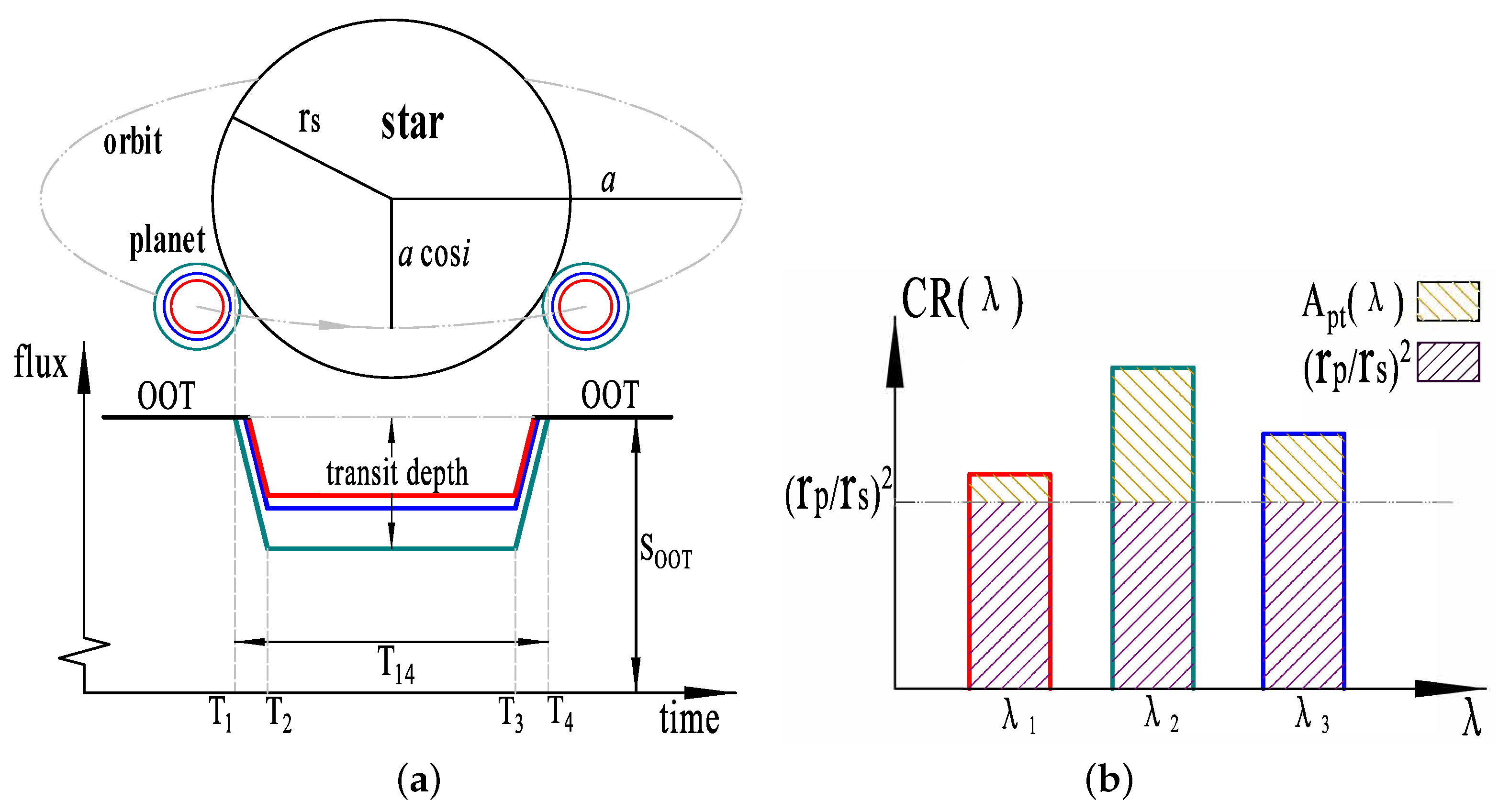
2.1. Transit-Spectroscopy Method
2.2. Transit-Spectroscopy Parameters
3. Optical Indices
3.1. Wavelength Coverage and F Number
3.2. Spectral Resolution and SNR
3.3. Telescope Aperture and Overall Throughput
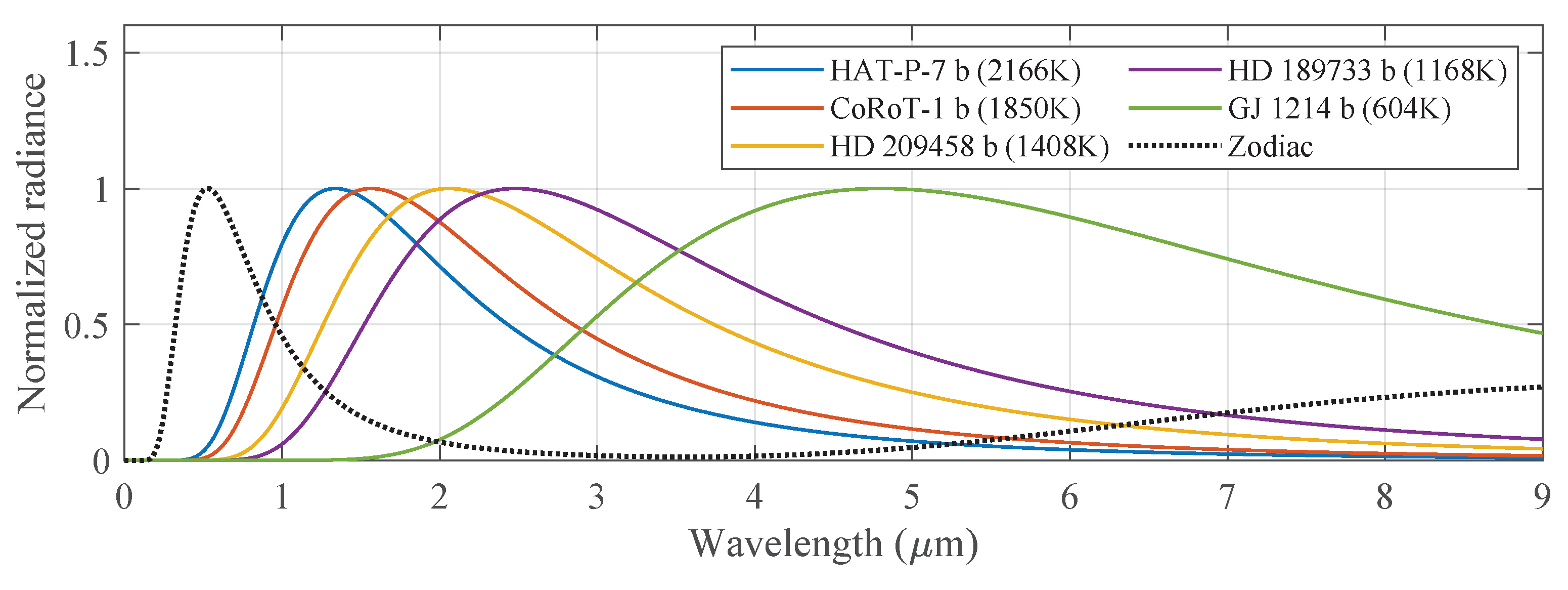
3.3.1. Stellar Signal
3.3.2. Total Noise
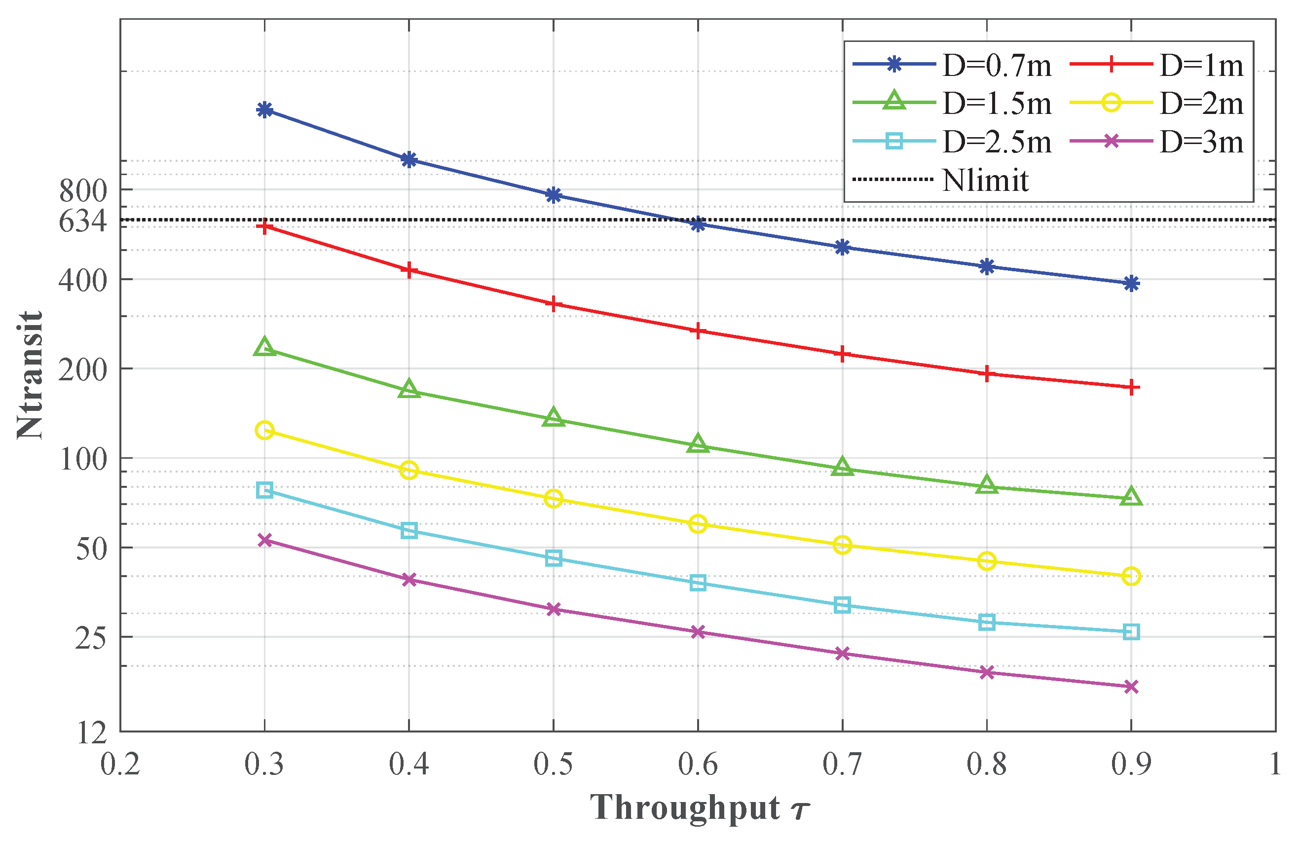
3.3.3. Selection of Telescope Aperture and Overall Throughput
3.4. Field of View
3.5. Optical Instrument Indices
4. Results of Optical-System Design and Simulation
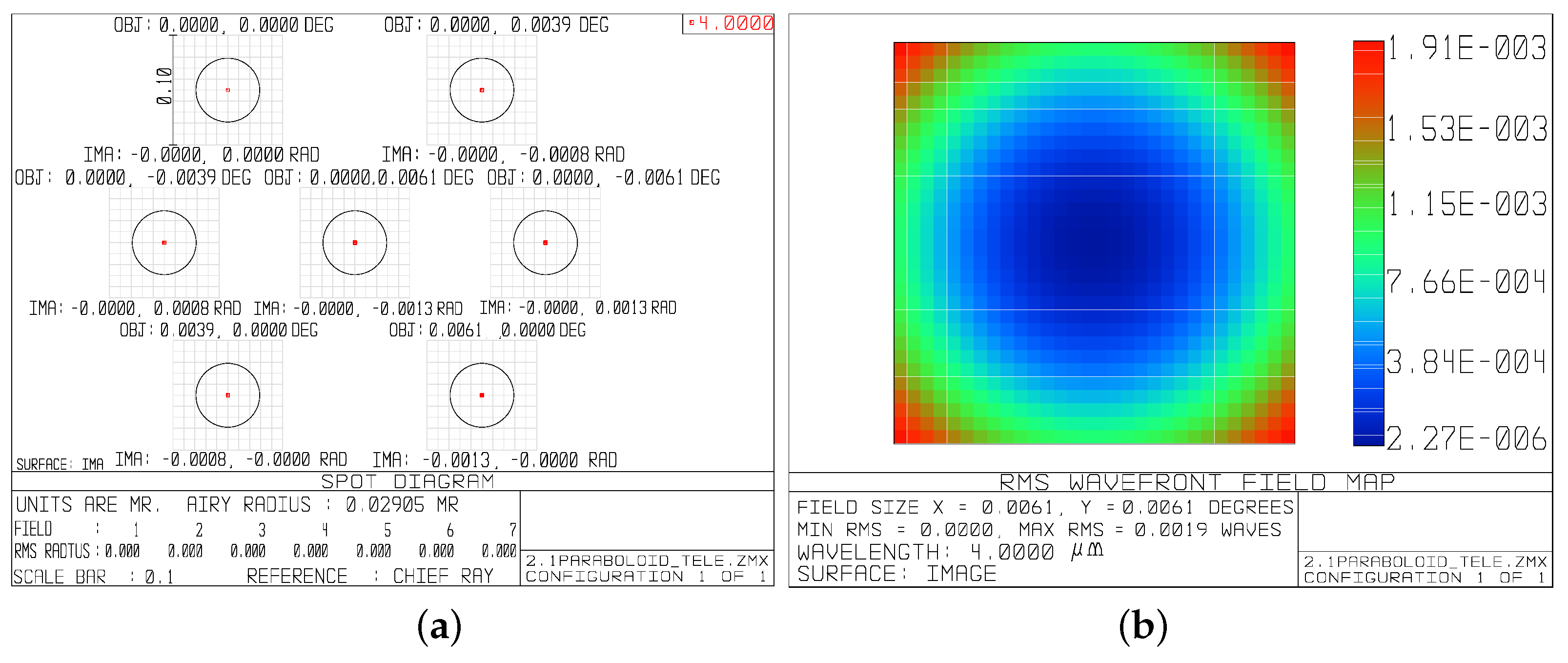
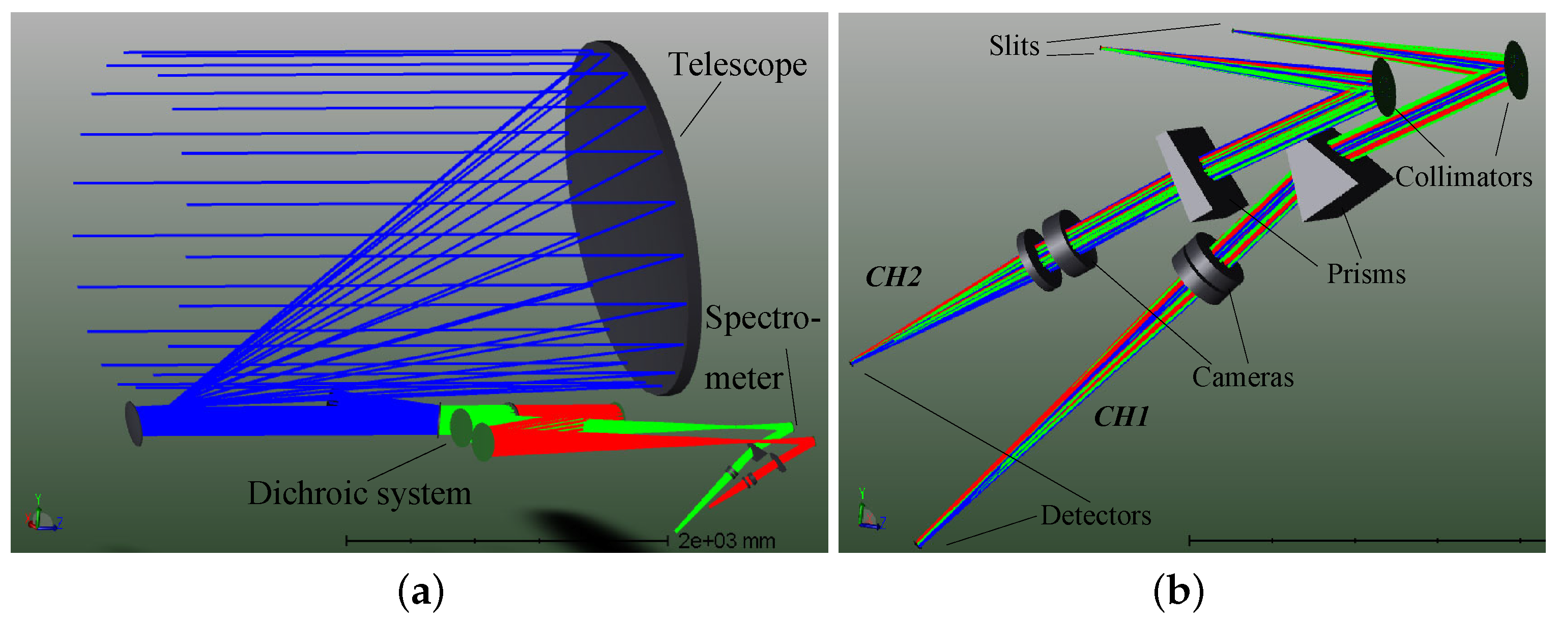
4.1. Telescope
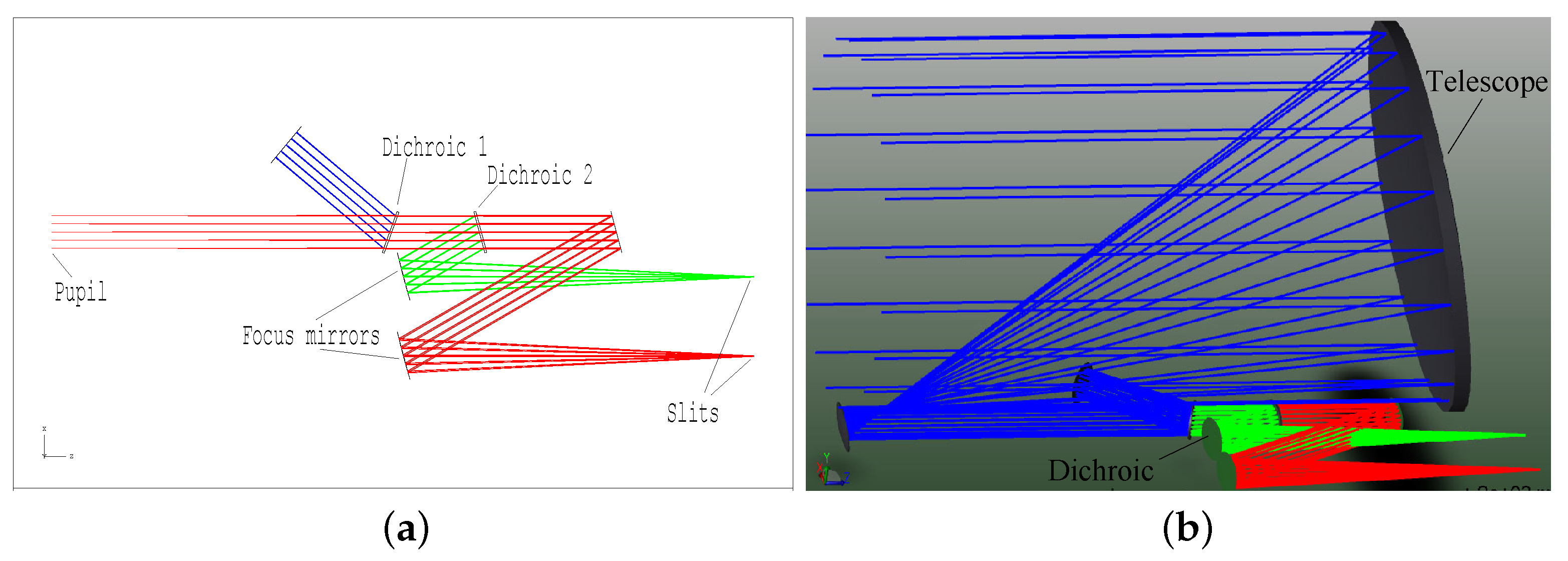
4.2. Dichroic System
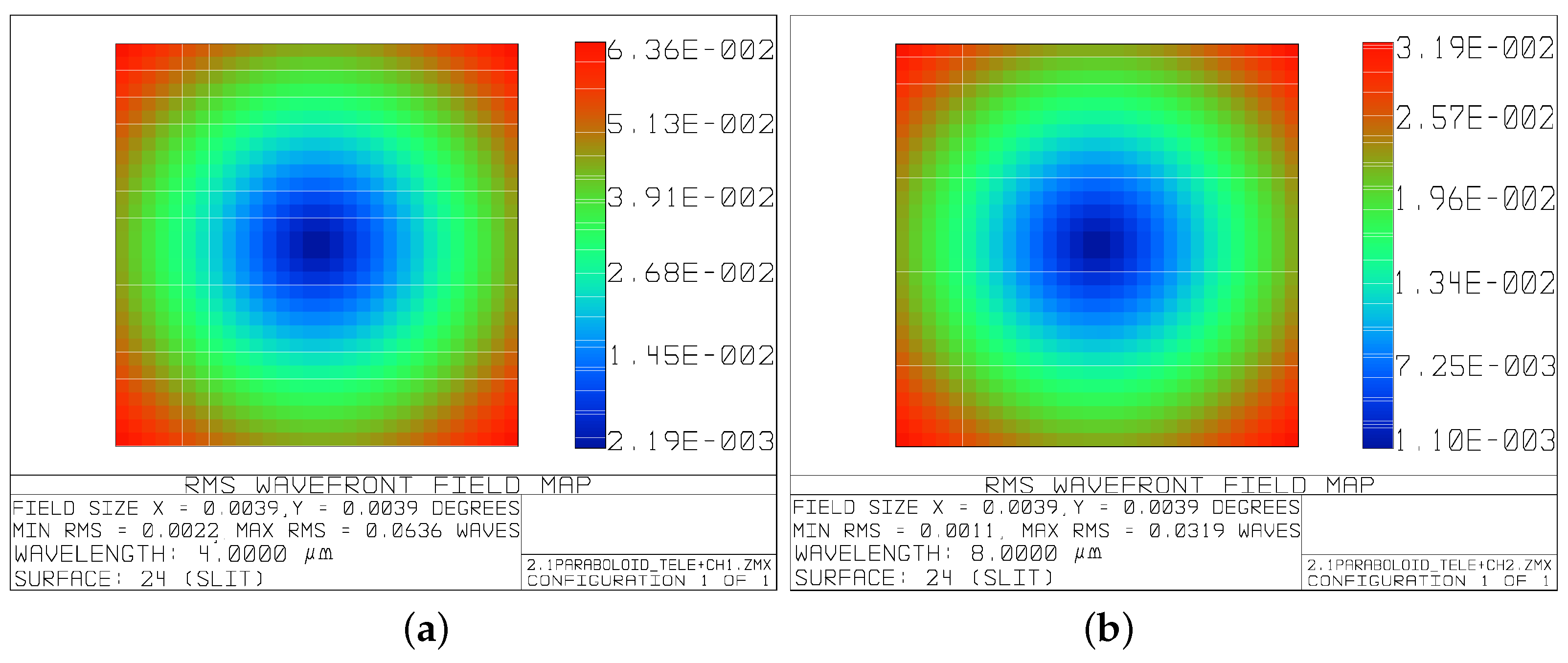
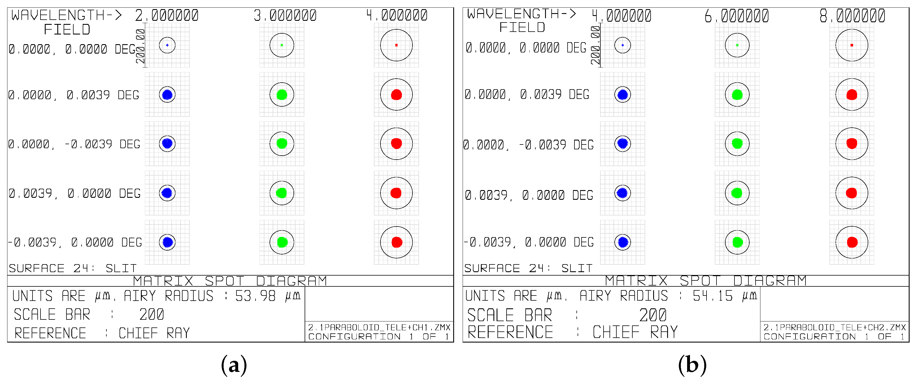
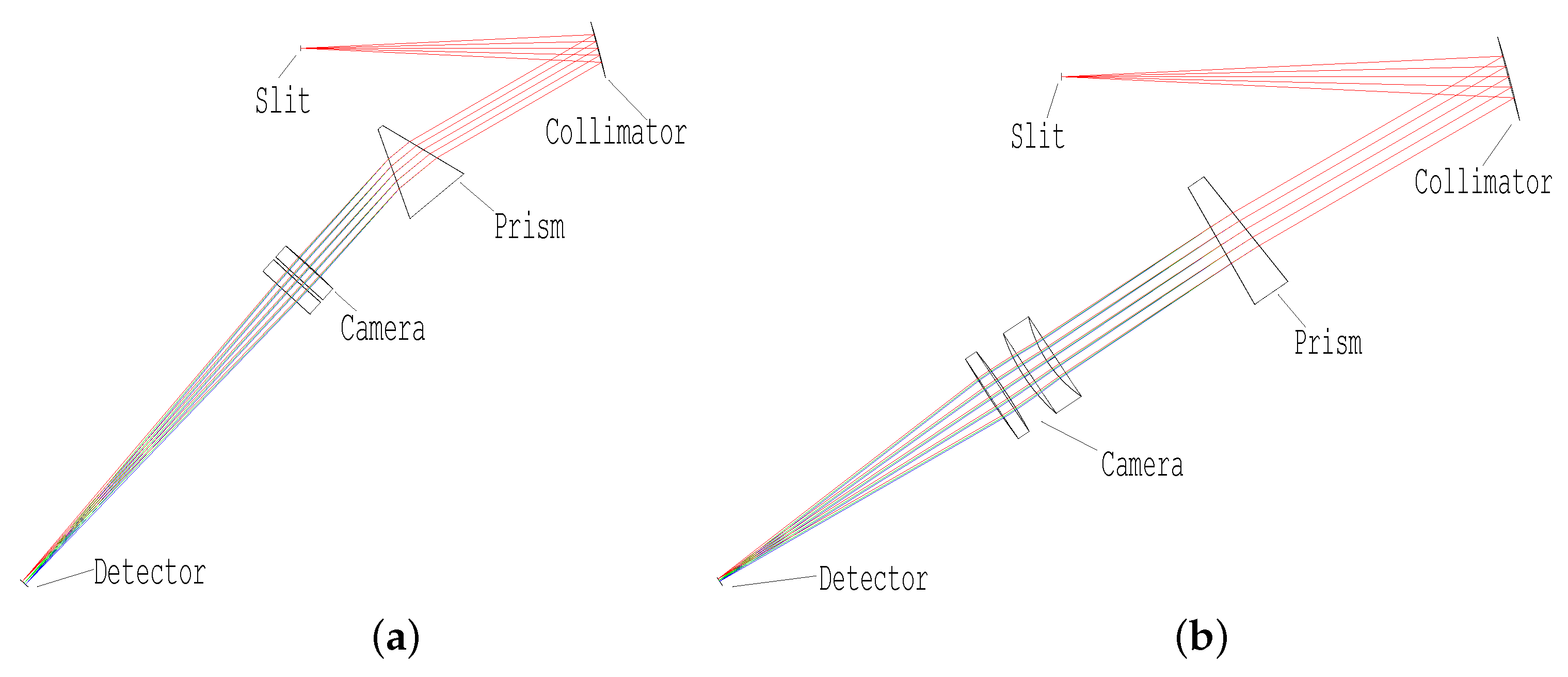
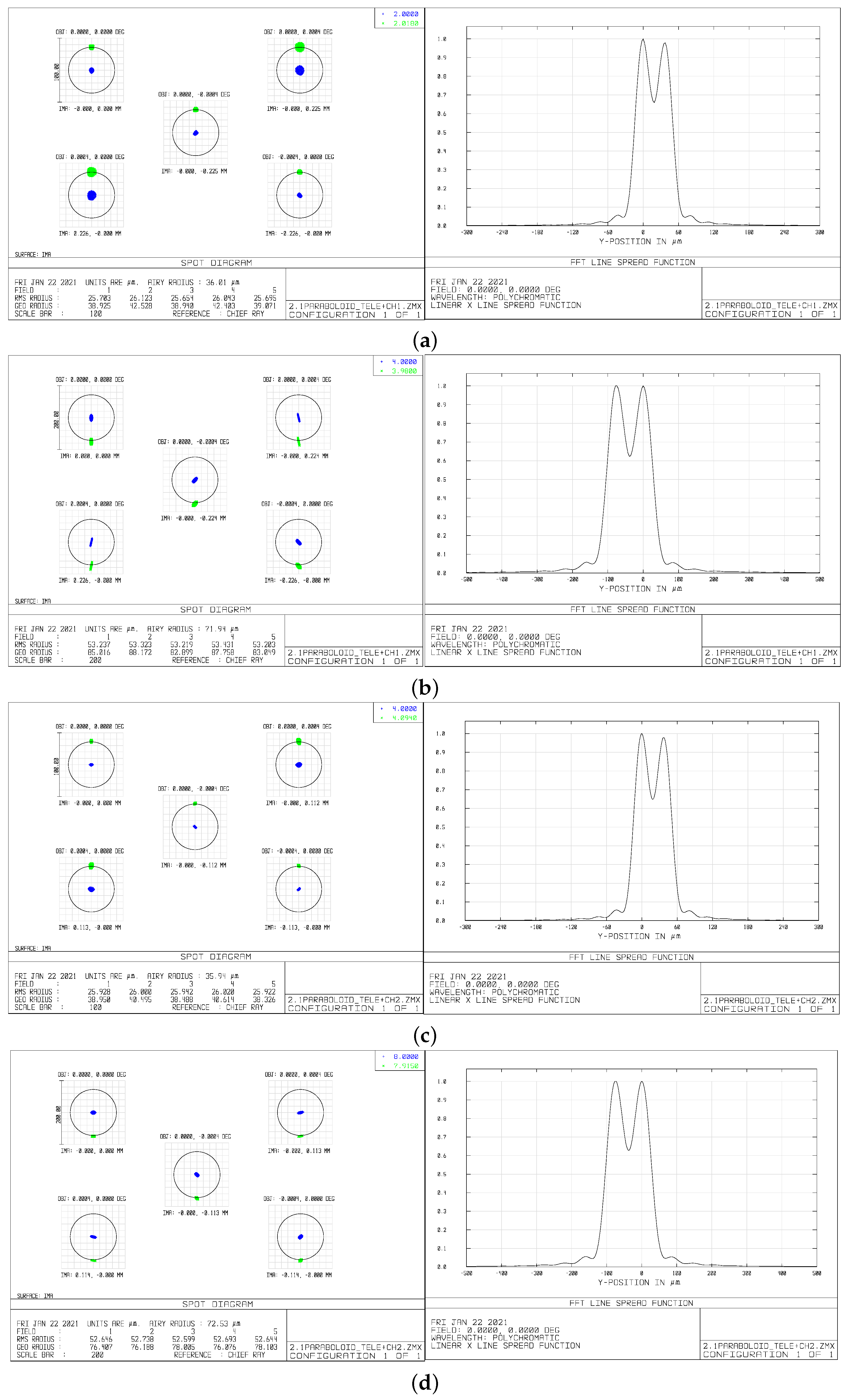
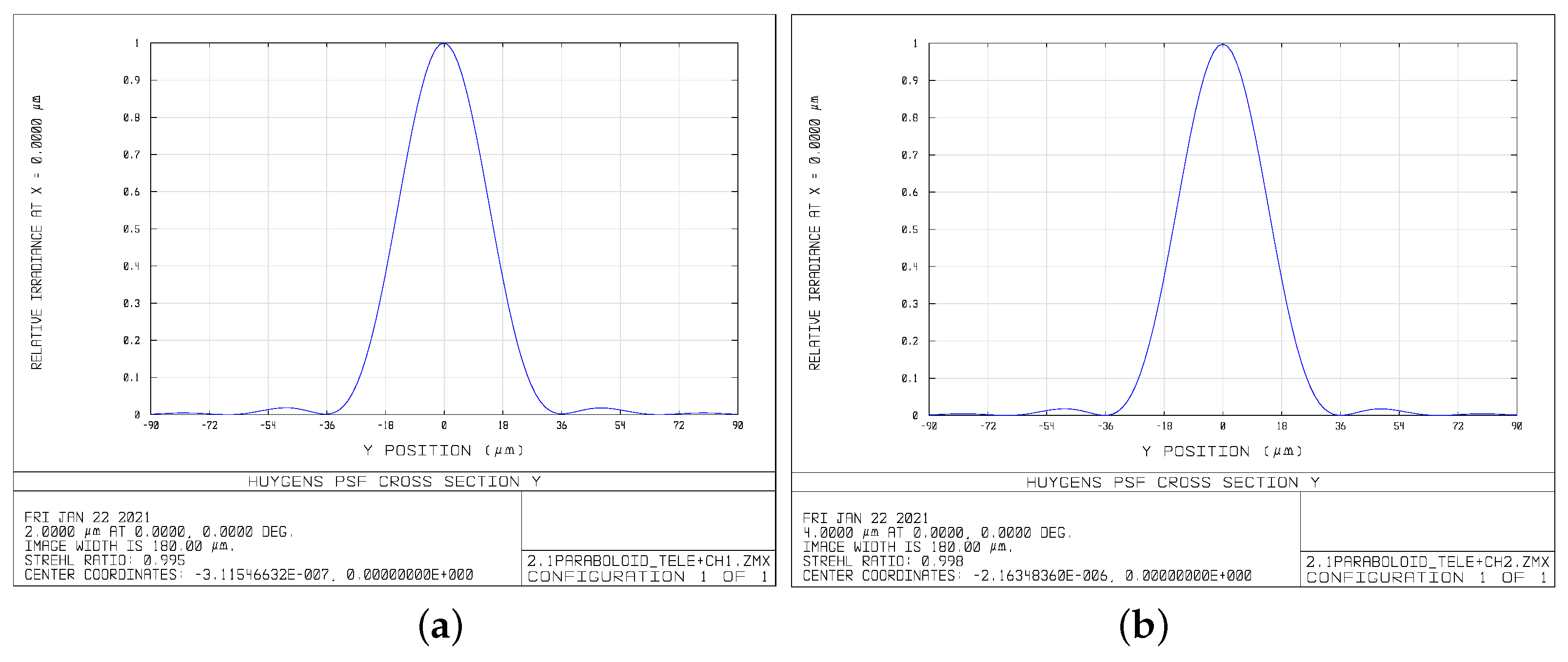
4.3. Infrared Spectrometer
5. Conclusions
Author Contributions
Funding
Institutional Review Board Statement
Informed Consent Statement
Data Availability Statement
Conflicts of Interest
References
- Kaltenegger, L.; Lin, Z. Finding Signs of Life in Transits: High-resolution Transmission Spectra of Earth-line Planets around FGKM Host Stars. Astrophys. J. Lett. 2021, 909, L2. [Google Scholar] [CrossRef]
- Morello, G.; Zingales, T.; Martin-Lagarde, M.; Gastaud, R.; Lagage, P.O. Phase-curve Pollution of Exoplanet Transmission Spectra. Astron. J. 2021, 161, 174. [Google Scholar] [CrossRef]
- Zhang, X. Atmospheric regimes and trends on exoplanets and brown dwarfs. Res. Astron. Astrophys. 2020, 20, 99. [Google Scholar] [CrossRef]
- Wang, F.; Fan, X.; Wang, H.; Shen, Y.; Pan, Y. Exoplanet detection methods and transit spectrometer equipment of astronomical telescopes. In Proceedings of the AOPC 2020: Optical Sensing and Imaging Technology, Beijing, China, 30 November–2 December 2020; Volume 11567, p. 558. [Google Scholar]
- Beichman, C.; Benneke, B.; Knutson, H.; Smith, R.; Lagage, P.O.; Dressing, C.; Latham, D.; Lunine, J.; Birkmann, S.; Ferruit, P.; et al. Observations of transiting exoplanets with the James Webb Space Telescope ( JWST). Publ. Astron. Soc. Pac. 2014, 126, 1134–1173. [Google Scholar] [CrossRef]
- Line, M.R.; Stevenson, K.B.; Bean, J.; Desert, J.M.; Fortney, J.J.; Kreidberg, L.; Madhusudhan, N.; Showman, A.P.; Diamond-Lowe, H. No thermal inversion and a solar water abundance for the hot Jupiter HD 209458b from HST/WFC3 spectroscop. Astron. J. 2016, 152, 203. [Google Scholar] [CrossRef]
- Encrenaz, T.; Tinetti, G.; Coustenis, A. Transit spectroscopy of temperate Jupiters with ARIEL: A feasibility study. Exp. Astron. 2018, 46, 31–44. [Google Scholar] [CrossRef]
- Tinetti, G.; Vidal-Madjar, A.; Liang, M.C.; Beaulieu, J.P.; Yung, Y.; Carey, S.; Barber, R.J.; Tennyson, J.; Ribas, I.; Allard, N.; et al. Water vapour in the atmosphere of a transiting extrasolar planet. Nature 2007, 448, 169–171. [Google Scholar] [CrossRef] [PubMed]
- Seager, S.; Sasselov, D.D. Theoretical transmission spectra during extrasolar giant planet transits. Astrophys. J. 2000, 537, 916–921. [Google Scholar] [CrossRef]
- Deming, D. Quest for a habitable world. Nature 2008, 456, 714–715. [Google Scholar] [CrossRef] [PubMed]
- Mugnai, L.V.; Pascale, E.; Edwards, B.; Papageorgiou, A.; Sarkar, S. ArielRad: The Ariel radiometric model. Exp. Astron. 2020, 50, 303–328. [Google Scholar] [CrossRef]
- Brown, T.M. Transmission Spectra as Diagnostics of Extrasolar Giant Planet Atmospheres. Astrophys. J. 2001, 553, 1006–1026. [Google Scholar] [CrossRef]
- Louie, D.R.; Deming, D.; Albert, L.; Bouma, L.G.; Bean, J.; Lopez-Morales, M. Simulated JWST /NIRISS Transit Spectroscopy of Anticipated Tess Planets Compared to Select Discoveries from Space-based and Ground-based Surveys. Publ. Astron. Soc. Pac. 2018, 130, 044401. [Google Scholar] [CrossRef]
- Berta, Z.K.; Charbonneau, D.; Désert, J.M.; Miller-Ricci Kempton, E.; McCullough, P.R.; Burke, C.J.; Fortney, J.J.; Irwin, J.; Nutzman, P.; Homeier, D. The flat transmission spectrum of the super-earth GJ1214b from Wide Field Camera 3 on the Hubble Space Telescope. Astrophys. J. 2012, 747, 35. [Google Scholar] [CrossRef]
- Sarkar, S. Exoplanet Transit Spectroscopy: Development and Application of a Generic Time Domain Simulator. Ph.D. Thesis, Cardiff University, Cardiff, UK, 2017. [Google Scholar]
- Rauer, H.; Gebauer, S.; Paris, P.V.; Cabrera, J.; Godolt, M.; Grenfell, J.L.; Belu, A.; Selsis, F.; Hedelt, P.; Schreier, F. Potential biosignatures in super-Earth atmospheres. Astron. Astrophys. 2011, 529, A8. [Google Scholar] [CrossRef]
- Seager, S.; Mallen-Ornelas, G. A Unique Solution of Planet and Star Parameters from an Extrasolar Planet Transit Light Curve. Astrophys. J. 2003, 585, 1038–1055. [Google Scholar] [CrossRef]
- Tinetti, G. The ARIEL Mission Proposal—A Candidate for the ESA M4 Mission. 2015. Available online: http://ariel-spacemission.eu/yellow-book-technical-documents (accessed on 30 March 2021).
- Encrenaz, T.; Tinetti, G.; Tessenyi, M.; Drossart, P.; Hartogh, P.; Coustenis, A. Transit spectroscopy of exoplanets from space: How to optimize the wavelength coverage and spectral resolving power. Exp. Astron. 2015, 40, 523–543. [Google Scholar] [CrossRef]
- Leinert, C.; Bowyer, S.; Haikala, L.K.; Hanner, M.S.; Hauser, M.G.; Levasseur-Regourd, A.C.; Mann, I.; Mattila, K.; Reach, W.T.; Schlosser, W.; et al. The 1997 reference of diffuse night sky brightness. Astron. Astrophys. Suppl. Ser. 1998, 127, 1–99. [Google Scholar] [CrossRef]
- Tinetti, G.; Drossart, P.; Eccleston, P. A chemical survey of exoplanets with ARIEL. Exp. Astron. 2018, 46, 135–209. [Google Scholar] [CrossRef]
- Barstow, M.A.; Barstow, J.K.; Casewell, S.L.; Holberg, J.B.; Hubeny, I. Evidence for an external origin of heavy elements in hot DA white dwarfs. Mon. Not. R. Astron. Soc. 2014, 440, 1607–1625. [Google Scholar] [CrossRef]
- Tinetti, G.; Encrenaz, T.; Coustenis, A. Spectroscopy of planetary atmospheres in our Galaxy. Astron. Astrophys. Rev. 2013, 21, 63. [Google Scholar] [CrossRef]
- Al-Refaie, A.F.; Changeat, Q.; Waldmann, I.P.; Tinetti, G. TauREx III: A fast, dynamic and extendable framework for retrievals. arXiv 2019, arXiv:1912.07759. [Google Scholar]
- Waldmann, I.P.; Rocchetto, M.; Tinetti, G.; Barton, E.J.; Yurchenko, S.N.; Tennyson, J. Tau-REx II: Retrieval of emission spectra. Astrophys. J. 2015, 813, 13. [Google Scholar] [CrossRef]
- Pan, Y.; Wang, H.; Jing, N.; Shen, Y.; Xue, Y.K.; Liu, J. Parameter selection and optical design of all-day star sensor. Acta Photonica Sin. 2016, 45, 0122002. [Google Scholar] [CrossRef]
- Sarkar, S.; Papageorgiou, A.; Pascale, E. Exploring the potential of the ExoSim simulator for transit spectroscopy noise estimation. In Proceedings of the Space Telescopes and Instrumentation 2016: Optical, Infrared, and Millimeter Wave, Edinburgh, UK, 26 June–1 July 2016; Volume 9904, p. 99043R. [Google Scholar]
- Pascale, E.; Waldmann, I.P.; MacTavish, C.J.; Papageorgiou, A.; Amaral-Rogers, A.; Varley, R.; de Foresto, V.C.; Griffin, M.J.; Ollivier, M.; Sarkar, S.; et al. EChOSim: The Exoplanet Characterisation Observatory software simulator. Exp. Astron. 2014, 40, 601–619. [Google Scholar] [CrossRef]
- Sarkar, S.; Madhusudhan, N.; Papageorgiou, A. JexoSim: A time-domain simulator of exoplanet transit spectroscopy with JWST. Mon. Not. R. Astron. Soc. 2020, 491, 378–397. [Google Scholar] [CrossRef]
- Sarkar, S.; Pascale, E. ExoSim: A novel simulator of exoplanet spectroscopic observations. Eur. Planet. Sci. Congr. 2015, 10, EPSC2015-187. [Google Scholar]
- Rein, H. A proposal for community driven and decentralized astronomical databases and the Open Exoplanet Catalogue. arXiv 2012, arXiv:1211.7121. [Google Scholar]
- Allard, F.; Homeier, D.; Freytag, B. Models of very-low-mass stars, brown dwarfs and exoplanets. Philos. Trans. R. Soc. A Math. Phys. Eng. Sci. 2012, 370, 2765–2777. [Google Scholar] [CrossRef]
- Mandel, K.; Agol, E. Analytic light curves for Planetary Transit Searches. Astrophys. J. 2002, 580, L171–L175. [Google Scholar] [CrossRef]
- McMurtry, C.; Lee, D.; Beletic, J.; Chen, C.Y.A.; Demers, R.T.; Dorn, M.; Edwall, D.; Fazar, C.B.; Forrest, W.J.; Liu, F.; et al. Development of sensitive long-wave infrared detector arrays for passively cooled space missions. Opt. Eng. 2013, 52, 091804. [Google Scholar] [CrossRef]
- Da Deppo, V.; Pace, E.; Morgante, G.; Focardi, M.; Terraneo, M.; Zocchi, F.E.; Bianucci, G.; Micela, G. A prototype for the primary mirror of the ESA ARIEL mission: Design and development of an off-axis 1-m diameter aluminium mirror for infrared space applications. In Proceedings of the Advances in Optical and Mechanical Technologies for Telescopes and Instrumentation III, Austin, TX, USA, 10–15 June 2018; Volume 1070632, p. 110. [Google Scholar]
- Da Deppo, V.; Middleton, K.; Focardi, M.; Morgante, G.; Pace, E.; Claudi, R.; Micela, G. Design of an afocal telescope for the ARIEL mission. In Proceedings of the Space Telescopes and Instrumentation 2016: Optical, Infrared, and Millimeter Wave, Edinburgh, UK, 26 June–1 July 2016; Volume 9904, p. 990434. [Google Scholar]
- Eccleston, P. ARIEL Payload Design Description; ARIEL-RAL-PL-DD-001; ARIEL Payload Consortium: Paris, France, 2017; Available online: https://arielspacemission.files.wordpress.com/2017/05/sci-2017-2-ariel.pdf (accessed on 30 March 2021).
- Morgante, G.; Terenzi, L.; D’Ascanio, D.; Eccleston, P.; Crook, M.; Hunt, T.; Da Deppo, V.; Focardi, M.; Micela, G.; Malaguti, G.; et al. Thermal architecture of the ESA ARIEL payload. In Proceedings of the Space Telescopes and Instrumentation 2018: Optical, Infrared, and Millimeter Wave, Austin, TX, USA, 10–15 June 2018; Volume 10698, p. 154. [Google Scholar]


| Exoplanet system | Super-Earth GJ 1214 b |
| Star features | M4.5 dwarf, 0.2213 R, 0.176 M, mag = 8.782 |
| Star Phoenix model | T = 3000 K, log g = 5.0, [Fe/H] = 0 |
| Planetary parameters | P = 1.58 d, 6.55 M, 2.84 R, T = 604 K, = 18 g/mol, T = 3161 s |
| A | 282.78 ppm |
| = 2 m) | CH1 | CH2 | Average | ||
|---|---|---|---|---|---|
| 0.3 | 0.573 | 149 | 0.704 | 99 | 124 |
| 0.4 | 0.671 | 109 | 0.819 | 73 | 91 |
| 0.5 | 0.751 | 87 | 0.919 | 58 | 73 |
| 0.6 | 0.831 | 71 | 1.015 | 48 | 60 |
| 0.7 | 0.898 | 61 | 1.095 | 41 | 51 |
| 0.8 | 0.93 | 53 | 1.173 | 36 | 45 |
| 0.9 | 1.019 | 47 | 1.239 | 32 | 40 |
| Exoplanets | ||
|---|---|---|
| hlHD209458b | 8.31227 × 10 | 1 |
| HD189733b | 5.16466 × 10 | 1 |
| WASP-13b | 6.21407 × 10 | 5 |
| WASP-34b | 9.91337 × 10 | 8 |
| HAT-P1b | 6.92584 × 10 | 10 |
| HAT-P26b | 1.00658 × 10 | 10 |
| WASP-12b | 7.61745 × 10 | 13 |
| Designation | FOV (arcsec) | Comments |
|---|---|---|
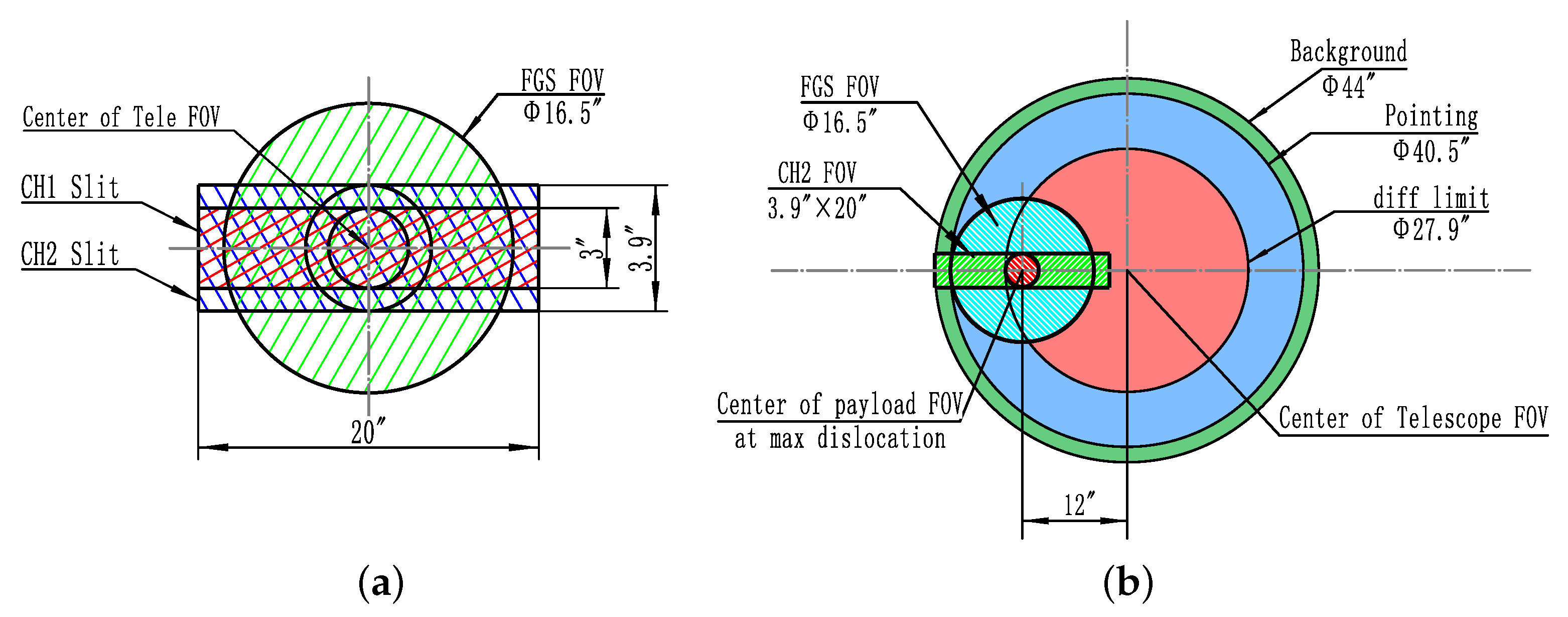
| CH1 | 3 × 20 | CH1 requires rectangular FOV with spectral direction of 3 and spatial direction of 20. |
| CH2 | 3.9 × 20 | CH2 requires rectangular FOV with spectral direction of 3.9 and spatial direction of 20. |
| Pointing system | 16.5 | Pointing system requires a 16.5 circular FOV. |
| Telescope with diffraction limit | 27.9 | Telescope is diffraction-limited within 27.9 to ensure well-resolved point-spread function (PSF) at the slit center. |
| Telescope with pointing acquisition | 40.5 | Telescope FOV within 41.5 allows for capturing a star and locating it in the slit center. |
| Telescope with background | 44 | Edge of telescope FOV is extended to 44 to capture slit background, demanding to be unvignetted to ensure that photons enter the slit without obstacles. |
| Parameter | Value |
|---|---|
| Wavelength coverage | Spectral: 2–8 μm; pointing: 0.5–2 μm |
| F number | 14.754 (2–4 μm); 7.377 (4–8 μm) |
| Resolving power | ∼100 (2–4 μm); ∼30 (4–8 μm) |
| SNR | ∼7 |
| Entrance aperture | ≥1.5 m |
| System throughput | ≥0.4 |
| FOV | Diffraction limited: 27.9; unvigneting: 44 |
| Parameter | Value |
|---|---|
| Wavelength coverage | 0.5–8 μm |
| FOV | Diffraction limited: 27.9, unvignetted: 44 |
| Collecting area | 3.46 m |
| Aperture | 2.1 m |
| Output-beam dimension | 0.2 m |
| Angular magnification | −10.5 |
| Parameters | CH1 (2–4 μm) | CH2 (4–8 μm) |
|---|---|---|
| Input F/# | f/10.8 | f/10.8 |
| Slit size | 0.33 mm × 2.2 mm | 0.43 mm × 2.2 mm |
| Prism material | CaF | CaF |
| Prism apex and incidence angle | 29.4° and 39.6° | 8.9° and 9.1° |
| Camera material | Silicon and germanium | CaF and ZnS |
| Airy radius in | 36 μm | 36 μm |
| PSF sampling and | 2 and 4 pix | 2 and 4 pix |
| Pixel scale | 0.12/pixel | 0.24/pixel |
| Pixel size | 18 μm | 18 μm |
Publisher’s Note: MDPI stays neutral with regard to jurisdictional claims in published maps and institutional affiliations. |
© 2021 by the authors. Licensee MDPI, Basel, Switzerland. This article is an open access article distributed under the terms and conditions of the Creative Commons Attribution (CC BY) license (https://creativecommons.org/licenses/by/4.0/).
Share and Cite
Wang, F.; Fan, X.; Wang, H.; Pan, Y.; Shen, Y.; Lu, X.; Du, X.; Lin, S. Optical System for the Transit Spectral Observation of Exoplanet-Atmosphere Characteristics. Appl. Sci. 2021, 11, 5508. https://doi.org/10.3390/app11125508
Wang F, Fan X, Wang H, Pan Y, Shen Y, Lu X, Du X, Lin S. Optical System for the Transit Spectral Observation of Exoplanet-Atmosphere Characteristics. Applied Sciences. 2021; 11(12):5508. https://doi.org/10.3390/app11125508
Chicago/Turabian StyleWang, Fang, Xuewu Fan, Hu Wang, Yue Pan, Yang Shen, Xiaoyun Lu, Xingqian Du, and Shangmin Lin. 2021. "Optical System for the Transit Spectral Observation of Exoplanet-Atmosphere Characteristics" Applied Sciences 11, no. 12: 5508. https://doi.org/10.3390/app11125508
APA StyleWang, F., Fan, X., Wang, H., Pan, Y., Shen, Y., Lu, X., Du, X., & Lin, S. (2021). Optical System for the Transit Spectral Observation of Exoplanet-Atmosphere Characteristics. Applied Sciences, 11(12), 5508. https://doi.org/10.3390/app11125508