Featured Application
Good mathematical modeling, which is used for prediction, is one of the most important elements of the predictive controller. Even the best simulation model only approximates the behavior of the object. In real applications, usage of the model generated based on simulation data may cause unstable controller behavior due to model mismatch. One method to avoid this inconvenience is to linearize the plant model based on data gained during real-time experiments, not based on simulation results. However, one should then take into account external disturbances, whose appearance causes deterioration of the obtained model quality and extends the time of reliable data collection. The proposed algorithm is a method for linearized plant model tuning based on real measurements. It allows for model identification on the basis of the simulation data and its tuning in order to fit experimental data. This method quickens the model identification procedure and allows for its usage in real MPC (Model Predictive Control) applications. It was proved that the tuned model usage leads to elimination of high-frequency oscillations during its validation based on real-time experimental data.
Abstract
Modeling is the most important component in predictive controller design. It should predict outputs precisely and fast. Thus, it must be adequate for the ship dynamics while having as simple a structure as possible. In a good ship model the standard deviation of a particular coefficient should not exceed of its value. Fitting the validation data to for short-term prediction and for long-term prediction is treated as a declared benchmark for model usage in ship course predictive controller. Regularization was proposed to ensure better state-space models to fit the real ship dynamics and more accurate standard deviation value control. Usage of the simulation results and real-time trials, as model estimation and validation data, respectively, during the identification procedure is proposed. In the first step a predictive linear model is identified conventionally, and then coefficients are regularized, based on the validation data, using a genetic algorithm. Particular linearized model coefficient standard deviations were decreased from more than of their values to approximately of them using genetic algorithm tuning. Moreover, the proposed method eliminated model output signal oscillations, which were observed during the validation process based on experimental data, gained during ship trials. Improved mapping of ship dynamics was achieved. Fit to validation data increased from and to and , respectively, for short-term and long-term prediction. The proposed method, which may be applied to real applications, is easily applicable and reliable. The tuned model is sufficiently suited to plant dynamics and may be used for future predictive control purposes.
1. Introduction
Modeling is the most important element in the model-based control techniques (e.g., Model Predictive Control). Its structure and way of identification depend on future applications (simulation or prediction), identification of data form (time- or frequency-domain), required model form (linear or nonlinear), and control type (discrete or continuous). The identification procedure is a demanding and time-consuming issue, and it should be done as precisely as possible. Therefore, it is still a growing branch in the field of control.
A ship is a highly nonlinear MIMO (Multiple Input Multiple Output) control object, which is characterized by large inertia and susceptibility to external disturbances such as wind and waves. There is a variety of developed ship models for the future control process. In the identification theory they are divided into two main groups: linear, which are accurate only near the set point, and nonlinear, which are proper for a wider ship speed range. Nonlinear ones are based on Kalman Filters [1], identified during model tests as the nonlinear mathematical model parameters [2], based on the backstepping procedure and the tuning design method using the complex model of Wagner–Smith [3]. These nonlinear models may be also based on neural networks, e.g., conventional [4] or probabilistic [5] ones. Linear ship models, for the future application in the ship automatic control system, are identified as a second-order linear Nomoto model based on zig-zag tests [6], input–output time domain data obtained from nonlinear ship dynamics, mathematical models [7], or as linear incremental models [8]. Synthesis of a predictive ship control system forces the use of a predictive plant model [9], which in practical applications is linearized to minimize the controller computational effort.
Deterministic artificial intelligence model reparametrization was presented in [10]. In this publication methodology, which automates control and eliminates tuning completely, the method is used to search for optimal parameter values and then to update the constants and constituent constants in rudder commands. Thus, this method may be an alternative for model predictive control because it easily uses artificial intelligence based reaparametrization instead of model parameters estimation.
System identification, applied to get a reliable ship maneuvering model, may be done in various configurations and based on a variety of algorithms. There are three types of models that are widely applied to the autonomous ship control: white-box (WBM), grey-box (GBM), and black-box (BBM) models. WBM is based on the deterministic equations and knowledge about the ship dynamics and kinematics. Due to nonlinearities, it is hard to identify a reliable ship’s WBM. BBMs are built only based on the input–output data sets. No knowledge about the system structure and parameters is required. This group of models includes neural models [11] and models established by using support vector machines [12]. Black-box modeling is useful when identifying nonlinear ship models. GBM’s structure is known, and parameters are estimated on the basis of gained input–output data. GBM combines advantages of the WBM and BBM. The Nomoto model is often used to model linearized ship dynamics for control purposes. Its coefficients are obtained via optimization procedures, e.g., genetic algorithms [13], particle swarm optimization [14], or frequency–domain identification procedure [15]. Nomoto models are valid for small rudder angles and low frequencies of rudder action [16]. They are also applicable for pod-driven USV [17], but they have a lower performance in output prediction compared to state-space models, whose identification procedure is based on prediction error minimization [8]. Therefore, state-space canonical GBMs are used in model-based control.
Researchers take notable effort to linearize ship dynamics. Proper linear vessel model identification requires a definition of the acceptable set-point deviations. They should be small enough to fulfill linear characteristic conditions and wide enough to allow for model identification. Thus, there is a need to acquire a large number of trials, where different amplitudes and sampling periods of pseudo-random input data are generated and output signal values are recorded. Moreover, all plant modes should be stimulated to get a reliable linear model. The majority of vessels are modeled using time-domain input–output data sets. There are two main methods to obtain a system response for the pseudo-random inputs. Data are obtained from real-time trials or on the basis of nonlinear ship dynamic simulators. The first method seems to be better because we identify real objects, not its mathematical model. However, it is really time-consuming and is a demanding task to obtain the necessary number of samples for the whole identification process. There is also a risk of external disturbances (wind, waves, and currents), which affect outputs. Even when tests are carried out in windless conditions, it is hard to stimulate all plant modes without passing ships into circulation. By having an available non-linear mathematical model, it is possible to simulate these trails, verify them during rapid prototyping, and obtain undisturbed input–output data sets. Although, identification is exposed to numerical errors, such as including some parts of the mathematical dependencies, instead of the actual ship dynamics. The family of the obtained models has significant parametric uncertainties, and individual coefficient values are identified with large standard deviations. In this paper, a regularization technique and model verification based on real-time ship trials is proposed to minimize drawbacks of model identification based on simulation results.
Regularization is a technique presented above and used during the identification procedure. It defines and takes into consideration model flexibility constants. Furthermore, regularization reduces model parametric uncertainties [18]. The higher the model order, the higher its flexibility. However, this leads to the increase in all parameter estimates of variance errors. Regularization leads to better control over parameters’ standard deviations and model matching. The main difficulty is to determine values of the bias error and variance coefficients. Their values define the Mean Square Error (MSE) of the estimated model parameters. Ljung in [18] proposes to use cross-validation, where bias error and variance are determined empirically. It is a time-consuming process where initial guesses may be not optimal ones. The second method to determine these coefficients is Marginalized Maximum Likelihood [18], where the regularization matrix should be parameterized empirically, and the likelihood function for their particular values should be written by hand. This method’s accuracy also depends on the personal experience and particular likelihood functions. The obtained parameter values, also in this case, may not be optimal.
There is a large group of heuristic algorithms that may be successfully used for optimization. Beyond them are, e.g., particle swarm optimization (PSO) and gravitational search algorithm (GSA). PSO may be used for multidimensional problems, and it ensures good convergence [19]. PSO and GSA algorithms, in their conventional form, are dedicated to finding the local minimum. Multilayered GSA proposed in [20] is dedicated to solving real-world problems. It has a better search performance, but its hierarchical structure is quite complicated, and the optimization procedure needs more computational power than when the genetic algorithm is used. Thus, it was proposed to use the conventional genetic algorithm.
The genetic algorithm (GA) is a part of the evolutionary algorithms group, which was developed to find approximate optimization of problem solutions. It simulates the heritage mechanism occurring in nature to find the global minimum in a short time period [21]. It is commonly applied in plant identification for the future control system. GAs are used for Linear Time Invariant (LTI) state-space helicopter model identification [22] and linear quadratic Gaussian (LQR) controller design. They also find applications in medical equipment control. Zermani and others [23] used GA to estimate NARMA input–output model humidification inside a newborn incubator. Modification of GA, called genetic programming (GP), is used in modeling and optimization of the direct methanol fuel cell [24]. Additionally, neural network structure, which is used for non-linear MIMO system modeling, may be determined with the use of GA. This approach is convenient when there is little or no knowledge about the object structure [25].
Genetic algorithms are also used in ship model identification procedures. Hidalgo et al. in [26] used a parallel genetic algorithm for finding high-speed ships’ transmittance parameters. They state the problem of reasonably searching and determining space combined with parallelization, which allows to achieve time constraints. They propose a nonlinear model, taking into account heaves caused by sea waves. A maneuvering non-linear mathematical model for ships was presented in [27]. Model coefficients were estimated on the basis of a classic genetic algorithm, optimizing the distance between the reference and recorded time histories. The devised model was created on the basis of a simulated zig-zag trial and was verified according to turning maneuver and Dieudonne spiral. The genetic algorithm is also used in ship rolling prediction models to automatically adjust least-squares support-vector machine (LSSVM) model parameters [28]. In the LSSVM algorithm the cost function is regularized by the least-squares function with equality constraints. Based on this method, a non-linear ship rolling prediction model was devised. Parameter identification of linear vessel models using gradient and genetic algorithms was presented in [29]. They proposed a way to solve the problem of varying ship parameter values identification in linearized models. Such a possibility is important for the synthesis and realization of control algorithms. The optimized Nomoto model, based on the Kempf trial simulated data, was created and presented.
Grey-box model (GBM) parameters are most often optimized with the use of evolutionary algorithms. The main advantage of this method is that all model parameters are estimated in one run. This is how the ship fuel consumption model [30] and hydraulic process of ship lock [31] were created. GA models are also used in maritime autonomous ship automatic control systems, where they are used for off-line path estimation based on stationary obstacles and on-line path modification to avoid collision [32]. Fitness function is then defined as an economic cost resulting from the shape of the ship’s own route. Ship mathematical models, with parameters optimized by GA, are also used in the automatic non-linear sliding mode control. Ship collision avoidance, taking into account ship maneuverability, was presented in [33], where steering course control parameters were optimized on-line by GA. Additionally, in [34] a nonlinear ship maneuvering model is combined with GA to obtain the optimum rudder angle command and length of target trajectory.
Results of the presented research show that it is justified to use the genetic algorithm in ship model identification and in autonomous ship control. In this paper, GA has been applied to optimize bias and variance error coefficients in the regularization procedure. The best trade-off between them is taken into account, which leads to the best model complexity. Combination of GA and regularization was developed, and it is presented in the paper in application to the training ship’s linear model identification. Results prove that it increases the quality of the model obtained from the simulation data fit to the actual ship input–output data. Thus, this method obtains a reliable linearized model, which will be less complicated and will need lower computing power than the non-linear model does, when applied in the model-based controller. In order to use the model in future MPC autonomous ship controllers, it was decided to identify discrete predictive GBM. This procedure introduces a lower probability of numerical errors related to the discretization of the continuous predictive model.
The rest of this paper is organized as follows. Section 2 describes the training ship, model identification procedure, and linear state-space model form. Section 2.3 presents the regularization procedure, and Section 2.4 shows how GA for regularization was used. Section 3 is devoted to the presentation of the results.
2. Materials and Methods
2.1. Training Ship—LNG Carrier
The training ship is an autonomous vessel used by the Foundation for Safety of Navigation and Environment Protection at Silm Lake, near Ilawa in Poland, during practical training and research activities. The LNG carrier, built at 1:24 scale, has 11.33 m length overall and is equipped with a modern electric drive. It consists of DC batteries, 2 pods located at stern, and a rotatable thruster combined with a tunnel thruster at bow. A picture of the ship is presented in Figure 1.
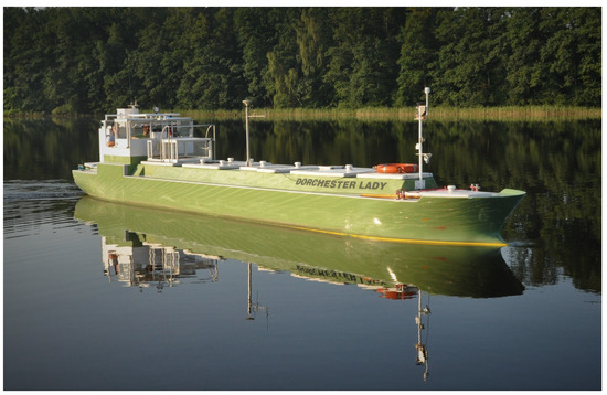
Figure 1.
LNG carrier—‘Dorchester Lady’.
Training vessel dynamics are highly non-linear and reflect the dynamics of a seagoing ship due to fulfillment of the laws of geometrical, kinematic, and dynamic similarity. Only the Reynolds number does not remain constant when comparing training ship to the real LNG carrier. Forces generated by the pods and interaction between them is described in detail in [35]. The whole training vessel model is presented in [36]. It is composed of three main subsystems describing hydrodynamic forces, forces from the propulsion system, and wind forces. It is a 3 DOF (degrees of freedom) nonlinear model, which is considered sufficient to describe surface ship motion. Roll, pitch, and heave are then omitted. In a general form, it is described by the following set of Equations (1)–(3):
where:
- m—ship mass,
- —the mass moment of inertia relative to the axis z,
- —surge, sway, roll
- —total longitudinal force,
- —total transversal force,
- —total torque.
Based on the above-mentioned mathematical model, the simulation test bed has been prepared. Individual subsystems have been implemented in MATLAB/Simulink software, and non-linear MIMO ship dynamics models have been created. It has been used as part of the hardware-in-the-loop system for quickly prototyping control algorithms. This system was also a data source for the linear model identification procedure with GA regularization.
2.2. Ship Linearized Model Identification
In model-based control strategies, such as Model Predictive Control (MPC), modeling is necessary to predict future plant outputs on the basis of past and current input signals. Thus, it determines the quality of designed control system. Fast, reliable, and being as accurate as possible are required. Ship dynamics are highly non-linear, full of cross-couplings between separate channels, and are difficult to model due to inertia and susceptibility to external disturbances. Most commonly known are non-linear ship models [1,5]. However, complications cause increases in computation time and demand for computational power, when determining optimal control values. Thus, there is a need to find simple and reliable linear model identification methodology.
A reliable linear model identification procedure requires:
- input–output data acquisition: identification trials should be recorded without external disturbances (e.g., wind, wave); all plant modes should be properly excited; ship should not enter into circulation; time-domain inputs should have different frequency and amplitude pseudo-random signals;
- model type selection: ship dynamics for the future control system are defined as a discrete state-space, polynomial, or transfer function model, which may be black-box (only the model order is specified) or grey-box (where initial guesses for coefficient values are provided);
- model order selection: the higher the model order is, the higher its flexibility, but there are also more parametric uncertainties in the obtained model; so there is a need to find a compromise between model flexibility and reliability;
- future model purpose definition: a good simulation model, in most cases of ship model identification, may have poor prediction, and vice versa, so one should specify the purpose of using the linear model.
- parameters estimation method selection: three methods are commonly used—subspace, prediction error minimization, and regularized reduction; the choice of parameter estimation method is strictly related to the future purpose of a model.
According to the described recommended model estimation sequence and experience governed during incremental model identification [8], a linear model was chosen. The gray-box state-space model, designed for prediction, identified with prediction error minimization estimation method, was chosen for future consideration.
State-Space Model Identification
A ship’s automatic course or trajectory tracking at constant speed, in the case of an azipod-powered vessel, can be reduced to a one-dimensional problem. In this type of control, course changes are realized by the pods’ angles of rotation change, while the propeller revolutions remain constant. The presented model will be used for a line-of-sight (LOS) trajectory tracking algorithm. The designed automatic control system has one controlled input (rotational speed r[deg/s]) and one output (pod angle of rotation [deg]). Due to this assumption, 3DOF single-input single-output (SISO) described by Equations (4) and (5) was identified. The mathematical model of the LNG Carrier ‘Dorchester Lady’ can be represented in state-space in form, which is schematically shown in Figure 2.
where:
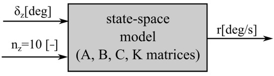
Figure 2.
Linear model structure schematic.
- —dynamic, input, output or sensor matrix,
- —noise component matrix,
- x, u, y—state, input and output vector,
- e—disturbance,
- —current time, next time moment.
The LNG carrier does not have direct feedthrough, which needs to be taken into account during the identification process. State-space model of canonical form, which guarantees observability, with white noise as the disturbance was identified. Viallon et al. [37] proved that the third-order polynomial model is sufficient to represent forces acting on a ship during normal maneuvers. They also include trajectory tracking, which is a future application for the MPC controller and will be built on the basis of the above-described model. In maritime autonomous surface ship (MASS) predictive control there is a need to predict future output instead of the force acting on the ship’s hull during simulation. Thus, it was decided to find empirically the state-space model order. As a first guess, the third order, based on [37], was analyzed. In the next step, the prediction based on the higher-order models was checked. A significant improvement in prediction was noticed after the model order increased to four, but no significant prediction improvement was noticed after further model order increase. Thus, it was decided to use the fourth-order state-space predictive model for further regularization. Individual matrices are described by Equations (6)–(9).
Matrices , and describe model with particular estimated parameters creating vector given by (10).
where: —estimated value of the particular parameter.
where: —parameterized model output prediction.
where:
- N—number of samples,
- —estimated model parameters vector.
According to Ljung [38], when taking into account prediction as the goal of a model, prediction error is determined by (11). In PEM, the quadratic norm of (11) acts as a cost function during the optimization procedure. In this approach, the variances of the parameter estimates may be very large because they are not included the cost function and optimization problem constraints. Cost function (12) is defined as the normalized sum of squared prediction errors. Vectors of the estimated parameter values are calculated during the optimization procedure that consist of minimizing the cost function.
A linear state-space predictive model was identified using the PEM method, based on computer simulation results. Pseudorandom pod angle of rotation sequences () were used as the source of input signals and were delivered to the inputs of the simulation model. They were used then as input data for identification. The ship’s rotational speed (), computed based on the nonlinear mathematical model, was registered and used as output data during the identification process.
2.3. Regularization Procedure
Regularization is a well-known technique used for presenting some initial knowledge in statistical and estimation problems. Ljung in [18] proved that this method may be applied to the identification problems, where an optimal regularization matrix, defined as the quadratic norm, is found. Mismatch of the estimated model may be described by two types of errors:
- –
- variance error: random error, representing uncertainty in the models’ parameter estimates;
- –
- bias error: systematic error, which represents model mismatch.
The model is then parameterized also with bias and variance errors. Perfectly matched parameters minimize the mean square error, described by: . The use of regularization allows for better control of the bias-to-variance ratio during model estimation. The cost function changes its form from (12) to (13) [38].
The standard cost function form is extended by two positively defined and R matrices. Matrix defines the effect of variance error traded for bias error. These two errors are connected together as follows: increase in the causes bias to increase and variance error to decrease. Thus, it improves the estimated model fit, while affecting deterioration of its parametric uncertainties.
R matrix is defined by weights and/or rotation of particular estimated model parameters ( vector values). It has an impact on penalty coefficients shaping and allows for constraint (e.g., model stability) to meet. It also allows for adding information about estimated parameters, such as the reliability of particular vector parameters.
Determination of regularization matrices is an empirical process [18]. It requires a priori knowledge () about estimated parameter values. Then represents the confidence of these parameters. However, the process of finding their values still requires carrying out cross-validation tests and having some guesses about parameter values, which is not trivial. The Marginalized Maximum Likelihood method [18] enforces matrix empirical estimation and allows for matrix parameterization, defined by (15). One may create matrix and write the likelihood functions for each parameter . There are some common ways to parameterize the impulse response of the FIR filter or the ARX model. However, none of them works properly with the state-space linearized ship dynamics model. Therefore, the regularization matrices have been defined using a genetic algorithm.
2.4. Genetic Algorithm for Regularization Matrix in Identification Representation
To determine regularization parameters, the matrix (15) and of the previously identified fourth-order state-space predictive model standard GA were used. It is an evolutionary method that allows for sub-optimal solutions to find and bypass the local minimum. Creating a new generation requires parent selection according to fitness function, selection, crossover, and mutation. The GA flowchart is presented in Figure 3. The initial population of individuals (P) is formulated in each time step according to Formula (16).
where:
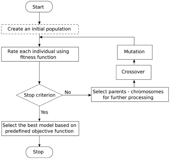
Figure 3.
Regularization genetic algorithm schematic.
- y—validation data output;
- —output of the real system.
Each individual () represents a possible solution to the stated problem, which is a set of parameters defined by matrix and . The fit function evaluates each obtained solution, and a new population is generated in five steps:
- Create an initial population—Real parameters ( and values) are coded as 13-bit chromosomes. and minimal values amount to , which is 100 times smaller than the estimated parameter magnitude and is treated as multiplication by zero. Their maximal values are, respectively, 200 for and 100 for , which is more than of the biggest estimated model coefficient value. The fit function is given by (17). The population reaches eight chromosomes. This parameter was obtained empirically. Bigger values caused only longer computation, without improving the results at the same time.
- Rate each individual using the fitness function—Fit value indicator describes how well the predicted model response () matches the measured data (y). Nonlinear ship model simulation data sets were used for input definition during the model identification process. Data measured during real-time lake trials was used in the model verification process when counting the fitness function value. The above-mentioned procedure was used in order to match the model as accurately as possible to the training ship dynamics. Moreover, during each individual rating process, the standard deviation (STD) of each model parameter was determined, and models whose STDs were bigger than of the identified parameter value were rejected. This elimiated unreliable models.
- Select parents—Chromosomes are selected with the use of stochastic methods. First of all, the algorithm rates individuals according to their survival curve. Next, it draws positions where the individuals will be placed in compliance with the pre-determined order. The total number of the individuals does not change.
- Crossover—Features of two parent chromosomes are passed on to descendants. Parental chromosomes exchange randomly chosen genes between each other and give two sets of genes for the descendants. Crossover probability () is equal to 0.25. A decrease in value leads to an unsuitable population with large STDs in it.
- Mutation—Mutation brings genes that do not come from any parent. It randomly changes one or more genes in the chromosome. Each gene of each individual in the population mutates independently of other genes with the probability () equal to 0.05. Too small a value of leads to a very small fitness function value. Its excessive increase causes a lack of algorithm convergence.
Genetic operators applied to the initial population create a new one. The fitness function rates it, and the next iteration of the algorithm begins. There are two termination conditions: fitness function value is bigger than , or its value does not change more than during the iteration. Compliance with the first condition means that a very good model has been identified. When the second condition is met there is no change due to regularization in the model identification procedure.
3. Results
The predictive model was identified on the basis of nonlinear LNG Carrier dynamics simulation data with the use of Matlab System Identification Toolbox. A large number of simulated time series was used to identify linear state-space models. However, these models were not reliable due to high standard deviations for some parameters. In Table 1, examples of model parameters and their STD values are presented. The STDs for parameters and are bigger than their values. Models like this occurred frequently during the classical identification process and were rejected.

Table 1.
Examples of unreliable model parameters and their STD values.
In order to use the model in the MPC algorithm it should be averaged, especially if a particular identified parameter varies more than . Example results of two models’ parameters whose STDs were smaller than of the coefficient value are presented in Table 2. In the fourth column averaged coefficients are presented. Figure 4 shows 5- (a) and 10-steps ahead (b) prediction of model 1, model 2, and the averaged model. The pseudo-random angle of pod rotation () with 5 s sampling time is an input signal (c). Quantitative analysis of the particular coefficients suggests the results are too widely spread. But when one has a look at the prediction results of the model compared against simulation validation data there are hardly any differences in the trials. Model 2 has more than 10 percentage points less fit. In the 10-step predicted response for model 2, high-frequency oscillation occurs, which should be eliminated before the model is applied to the MPC algorithm.
Table 2.
Examples of identified models and the average model comparison.
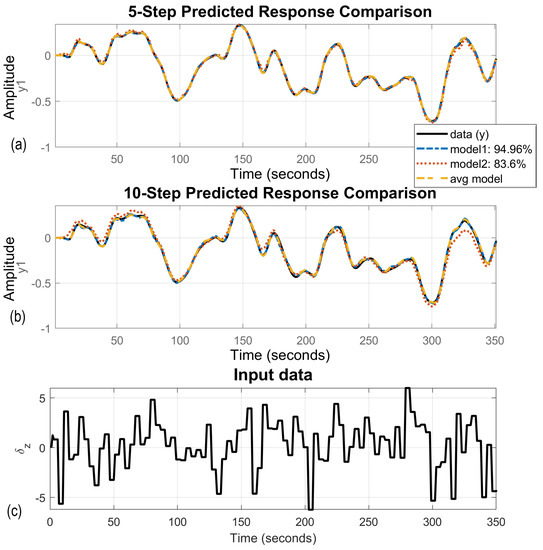
Figure 4.
Examples of identified model predictions based on simulated validation data. (a) 5-steps ahead prediction, (b) 10-steps ahead prediction, (c) validation data sequence.
In the second stage of model verification, real-time trials on Silm Lake were done. Pseudo-random pod angles of rotation are input signals that, combined with outputs, create validation data sets. Conventionally identified models generated oscillations during validation. This is presented in Figure 5. Model 1 and the averaged model produced high-frequency oscillations with magnitude within of the output signal value. However, oscillations that occurred during model 2 validation process were bigger than the output signal amplitude multiplied by 15. This means this model is useless for all prediction horizons. Moreover, the fit of the model outputs to the validation data was less than for model 1 and reached for the averaged model. Using them in the prediction process will lead to significant errors. Therefore, GA regularization was applied during the model identification process. Figure 6 presents an enlarged section (50 seconds of the trial) cut of the graph presented in Figure 5. It shows that model 1 and the averaged model were not good enough, but also were not completely useless as model 2.
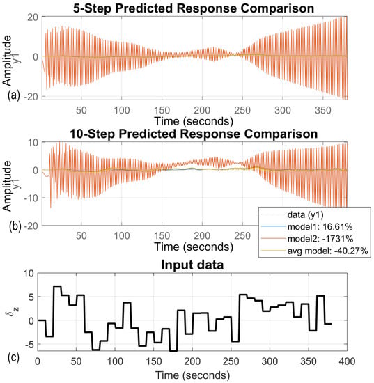
Figure 5.
Examples of model predictions based on real-time lake validation data; (a) 5-steps ahead prediction, (b) 10-steps ahead prediction, (c) validation data sequence.
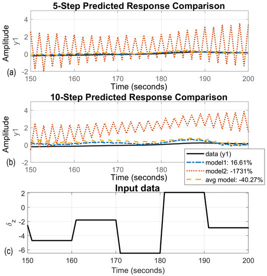
Figure 6.
Examples of model predictions based on real-time lake validation data, magnified figure. (a) 5-steps ahead prediction, (b) 10-steps ahead prediction, (c) validation data sequence.
Fifteen real-time lake experiments were conducted, in which pseudorandom pod angles of rotation sequences were pod command signals. The ship’s rotational speed was recorded during the whole research experiment. Sequences of pod angles of rotation combined with the ship’s rotational speed were then used as validation data. Models were identified on the basis of the simulation results and regularized, using GA, on the basis of the real-time ship trial results. Exemplary model parameters, their STD values, and regularization parameters for each coefficient () are compiled in the Table 3. The model was identified with . It gave reliable results with STDs less than of the coefficient values. Figure 7 presents GA model fit to the validation data obtained during the real-time lake trial (c). There were no high-frequency oscillations in the time trials. For 5-step ahead prediction (a) results fit the validation data and reached , which gives very good prediction. For 10-step ahead (b) the fit decreased and gave a reliable model with fit equal to , which can be used in the MPC controller. Prediction of horizon elongation led to decreased fit. The model that reflects ship dynamics and whose fit function is greater than is good enough to be a component of the MPC. Figure 8 and Figure 9 illustrate, respectively, the regularized GA model and conventional model 5- and 10-step ahead predictions based on real-time lake validation data. These data, combined with the averaged non-regularized model fit, are presented in Table 4. In both cases prediction of horizon elongation caused the fit to decrease. In the conventionally identified model, two high-frequency oscillations make its application to MPC impossible. In the GA model the fit was greater and the output signal was smooth. Moreover, the GA model fitness function had about bigger value, which proves the legitimacy of using the GA algorithm during the identification process. In Table 5 the percent improvement of the prediction ability of the tuned model is presented, compared to the reference values, guaranteeing the performance of the MPC controller and the non-regularized model prediction ability.
Table 3.
Example of GA tuned model parameters and their STD values.
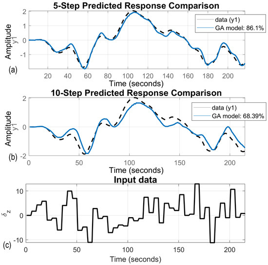
Figure 7.
Examples of regularized GA model prediction based on real-time lake validation data; (a) 5-steps ahead prediction, (b) 10-steps ahead prediction, (c) validation data sequence.
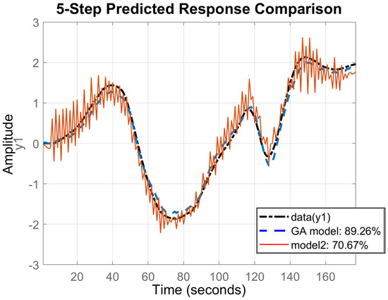
Figure 8.
Regularized GA model and conventional model 5-step ahead prediction comparison based on real-time lake validation data.
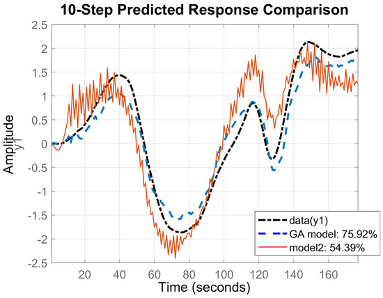
Figure 9.
Regularized GA model and conventional model 10-step ahead prediction comparison based on real-time lake validation data.
Table 4.
Prediction ability of the GA regularized model combined with the averaged non-regularized model.
Table 5.
Percent improvement of the prediction ability of the tuned model, compared to the reference values guaranteeing MPC controller performance and non-regularized model prediction ability.
Table 6 presents the percentage STD values in relation to the model parameter values. They should not exceed in order to get a good model, and exceeding the value of makes the model unreliable. The GA tuning method decreased their percentage values, and only one of them was bigger than but still remained less than . These percentage values guaranteeing model reliability were not obtained during the conventional identification procedure. A significant improvement in the quality of the model was achieved during GA tuning for – coefficients. Percentage STD values for the rest of the coefficients were comparable in both the conventional identification and GA tuning method.
Table 6.
Percentage STD values in relation to the model parameter values.
Model division for future MASS predictive control requires averaging the estimated parameters values. During the identification procedure we obtained one model for each data set, and the controller needs one model for each working point. Figure 10 presents results of averaging the parameters. The model output was compared with validation lake trial data. The model fit decreased as the prediction horizon elongated. The model fit for short-term prediction (a) reached almost and fell to almost for mid-term prediction (b). Long-term prediction (c) is rarely used in MASS control systems. From the obtained result, the mapping rotational speed changing tendency was sufficient. Results presented in Figure 10 prove that it is justified to regularize the identified model using real validation data. This avoids the occurrence of high-frequency disturbances related to the identification of the mathematical relationships that constitute the mathematical model, instead of the dynamics of the ship.
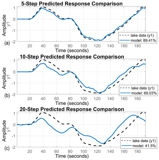
Figure 10.
Regularized GA model: 5-, 10-, and 20-step prediction comparisons based on real-time lake validation data; (a) 5-steps ahead prediction, (b) 10-steps ahead prediction, (c) 20-steps ahead prediction.
4. Discussion
A great variety is observed in ship dynamics modeling. The situation is much easier when we deal only with simulations. However, it is complicated when the controller is applied to a real plant/floating ship. It turns out that there were unmodeled elements of the object dynamics. Failure to take them into account in the predictive model causes the oscillations that were observed during experimental data validation. The obtained results proved this theory and showed that there was a perfect fit to the simulation validation data and a poor fit to the experimental validation data. In the case of simulating validation data, no deterioration in the prediction quality was observed along with the length of the prediction horizon. Nevertheless, such a deterioration was recorded during model validation based on real-time experimental data gained during lake trials. It can be concluded that the input data used for linearization are much more important than the structure of the model itself. The presented method allows for maintaining a simple structure of the model while tuning its parameters to the real plant/ship.
During identification based on simulation data, a linear model is created by mapping mathematical, not physical, relationships. Not all cross-couplings between several channels are taken into account. Thus, the proposed method gives the opportunity to take into account the most important, from the prediction point of view, cross-couplings and allows for the model to be tuned to the real dynamics of the object, not only its mathematical description.
Widely used in ship control theory and applications, the Nomoto model is insufficient for prediction purposes. Hence, there is a need to develop a different methodology for building a simple predictive ship model. The proposed algorithm for linear model identification in state-space combined with GA tuning is the answer to this need in real applications.
Neural-network and LSSVM models are vert extended ones. Their identification is time consuming, and usage in MPC is limited, due to the computation power of the on-board ship controller. The proposed model is a very simple, linear state-space one, which is easy to implement in real-world applications and may be used in MASS predictive control systems.
5. Conclusions
Model Predictive Controller design requires incorporating good ship dynamics in the predictive model. A large amount of data for the identification procedure may be obtained in two ways: during non-linear ship model simulations or during real-time lake trials. We should obtain reliable data where all modes of the plant will be excited. Lake identification trials should be done without any disturbances such as wind, waves, and current. There is also difficulty with all modes of excitation without bringing the training ship into circulation. These trials are time-consuming and susceptible to severe errors. Thus, a method that combines simulation test and real-time trial validation data is presented. This method reduces the number of lake trials by about four times and gives acceptable results, indicating it is a good predictive model for further usage.
Regularization is a straightforward procedure allowing for better control of the identification process. It allows for minimizing the standard deviations of particular coefficients and maximizing fitness function values. The GA procedure quickens matrix and parameters search. It also brings their sub-optimal values, which are hard to find during conventional computations. Use of modern computers, with high computation power, allows for on-line parameter search. The obtained model may be modified during automatic MPC control, when ship parameters are changing, for example during underway replenishment, when the ship’s metacentric height, draught, and load displacement change.
Overall, the GA and conventional model qualities are measured by acceptable STDs and the validation fitness function value. The model whose coefficient STDs are bigger than of their value is rejected. They are treated as unreliable. In addition, models causing high-frequency oscillations in the output signals are useless. GA regularization prevents the appearance of the above-mentioned unwanted STDs and oscillations. Parameters such as dynamic, output, and noise component matrices, whether or not GA regularization has been used, have STDs less than . However, input matrix coefficients, when identification was done on the basis of the simulation data, had STDs exceeding even of the coefficient value. GA regularization usage minimizes them to the values amounting to a small percent. Only the STD for the coefficient () exceeded , but it did not reach , which is acceptable for a single parameter for MPC design purposes. Moreover, use of GA regularization prevents oscillations in output signals. Therefore, the method presented in this paper can be used to predict future plant outputs for MPC.
The minimal fit to validation data, in order to get a reliable predictive model for future control purposes, was equal to for short-time and for long-time predictions. GA regularization resulted in a model with predictive capabilities exceeding the reference short- and long-time prediction ability by 9 and 11 percentage points, respectively. The non-tuned model did not meet the reference values. Thus, significant prediction performance was achieved, which reached and percentage points for short- and long-time predictions, respectively.
This algorithm is a good tool for identification of the real plant indirectly based on simulation data associated with real experiments. It may be used not only for ships, but for all nonlinear and nonholomical control objects. It gives a reliable prediction model, which may be applied to the MPC algorithm for future automatic control systems.
Funding
The project was financed within the program of the Polish Ministry of Science and Higher Education called “Regional Initiative of Excellence” for the years 2019–2020, project number 006/RID/2018/19 financing amount 11,870,000 PLN.
Institutional Review Board Statement
Not applicable.
Informed Consent Statement
Not applicable.
Data Availability Statement
Data available on request due to privacy.
Conflicts of Interest
The author declares no conflict of interest.
Abbreviations
The following abbreviations are used in this manuscript:
| BBM | Black-box model |
| DC | Direct current |
| DOF | Degrees of freedom |
| GA | Genetic algorithm |
| GBM | Gray-box model |
| GP | Genetic programming |
| GSA | Gravitational Search Algorithm |
| LNG | Liquid Natural Gas |
| LOS | Line-of-sight |
| LSSVM | Lest-Squares Support-Vector Machines |
| LTI | Linear Time Invariant |
| MASS | Maritime Autonomous Surface Ship |
| MIMO | Multiple Input Multiple Output |
| MPC | Model Predictive Control |
| MSE | Mean Square Error |
| NARMA | Nonlinear Autoregressive Moving-average |
| PEM | Prediction Error Minimization |
| PSO | Particle Swarm Optimization |
| SISO | Single Input Single Output |
| STD | Standard deviation |
| USV | Unmanned Surface Vessel |
| WBM | White-box model |
References
- Shi, C.; Zhao, D.; Peng, J.; Shen, C. Identification of ship maneuvering model using extended Kalman Filters. Mar. Navig. Saf. Sea Transp. 2009, 3, 105–110. [Google Scholar]
- Skjetne, R.; Smogeli, Ø.N.; Fossen, T.I. Identification of ship maneuvering model using extended Kalman FiltersA nonlinear ship manoeuvering model: Identification and adaptive control with experiments for a model ship. Model. Identif. Control. 2004, 25, 3–27. [Google Scholar] [CrossRef]
- Casado, M.H.; Ferreiro, R. Identification of the nonlinear ship model parameters based on the turning test trial and the backstepping procedure. Ocean. Eng. 2005, 32, 1350–1369. [Google Scholar] [CrossRef]
- Dai, S.L.; Wang, C.; Fuo, L. Identification and learning control of ocean surface ship using neural networks. IEEE Trans. Ind. Inform. 2012, 8, 801–810. [Google Scholar] [CrossRef]
- Araghi, L.F.; Khaloozade, H.; Arvan, M.R. Ship identification using probabilistic neural networks (PNN). In Proceedings of the International Multiconference of Engineers and Computer Scientists, Hong Kong, China, 18–20 March 2009; pp. 18–20. [Google Scholar]
- Artyszuk, J. A study on the identification of the second-order linear Nomoto model from the zigzag test. Zesz. Nauk. Akad. Morskiej Szczecinie 2018, 53, 59–67. [Google Scholar]
- Gierusz, W. Synteza Wielowymiarowych Ukladow Sterowania Precyzyjnego Ruchem Statku z Wykorzystaniem Wybranych Metod Projektowania Ukladow Odpornych; Akademia Morska w Gdyni: Gdynia, Poland, 2004. [Google Scholar]
- Miller, A. Identification of a multivariable incremental model of the vessel. In Proceedings of the 21st International Conference on Methods and Models in Automation and Robotics (MMAR), Miedzyzdroje, Poland, 29 August–1 September 2016; pp. 219–224. [Google Scholar]
- Khaled, N.; Pattel, B. Practical Design and Application of Model Predictive Control: MPC for MATLAB® and Simulink® Users; Butterworth-Heinemann: Oxford, UK, 2018. [Google Scholar]
- Sands, T. Development of Deterministic Artificial Intelligence for Unmanned Underwater Vehicles (UUV). J. Mar. Sci. Eng. 2020, 8, 578. [Google Scholar] [CrossRef]
- Rajesh, G.; Bhattacharyya, S. System identification for nonlinear maneuvering of large tankers using artificial neural network. Appl. Ocean. Res. 2008, 30, 256–263. [Google Scholar] [CrossRef]
- Wang, X.; Zou, Z.; Ren, R.; Cai, W. Black-box modeling of ship maneuvering motion in 4 degrees of freedom based on support vector machines. Ship Build. China 2014, 55, 147–155. [Google Scholar] [CrossRef]
- Marcjan, K.; Gucma, L. Optimizing the parameters of the simplified hydrodynamic model using genetic algorithms for the prediction marine systems use. Zesz. Nauk. Akademia Morska w Szczecinie 2010, 20, 87–91. [Google Scholar]
- Chen, Y.; Song, Y.; Chen, M. Parameters identification for ship motion model based on particle swarm optimization. Kybernetes 2010, 39, 871–880. [Google Scholar] [CrossRef]
- Ghorbani, M. Line of sight waypoint guidance for a container ship based on frequency domain identification of Nomoto model of vessel. J. Cent. South Univ. 2016, 23, 1944–1953. [Google Scholar] [CrossRef]
- Xing, D.; Zhang, L.; Wang, X.; Ma, R. Nonlinear cloud model control for ship steering based on genetic algorithms. In Proceedings of the 2011 International Conference on Consumer Electronics, Communications and Networks (CECNet), Xianning, China, 11–13 March 2011; IEEE: Piscataway, NJ, USA, 2011; pp. 499–502. [Google Scholar]
- Mu, D.; Wang, G.; Fan, Y.; Bai, Y. The Response Model of Modeling and Identification of Podded Propulsion Unmanned Surface Vehicle. J. Comput. 2017, 28, 125–138. [Google Scholar]
- Ljung, L.; Singh, R.; Chen, T. Regularization features in the system identification toolbox. IFAC-PapersOnLine 2015, 48, 745–750. [Google Scholar] [CrossRef]
- Cao, Y.; Zhang, H.; Li, W.; Zhou, M.; Zhang, Y.; Chaovalitwongse, W.A. Comprehensive learning particle swarm optimization algorithm with local search for multimodal functions. IEEE Trans. Evol. Comput. 2018, 23, 718–731. [Google Scholar] [CrossRef]
- Wang, Y.; Gao, S.; Zhou, M.; Yu, Y. A multi-layered gravitational search algorithm for function optimization and real-world problems. IEEE/CAA J. Autom. Sin. 2020, 8, 94–109. [Google Scholar] [CrossRef]
- Davis, L. Handbook of Genetic Algorithms; Van Nostrand Reinhold: New York, NY, USA, 1991. [Google Scholar]
- Wang, T.; Chen, Y.; Liang, J.; Wu, Y.; Wang, C.; Zhang, Y. Chaos-genetic algorithm for the system identification of a small unmanned helicopter. J. Intell. Robot. Syst. 2012, 67, 323–338. [Google Scholar] [CrossRef]
- Zermani, M.A.; Feki, E.; Mami, A. Application of Genetic Algorithms in identification and control of a new system humidification inside a newborn incubator. In Proceedings of the 2011 International Conference on Communications, Computing and Control Applications (CCCA), Hammamet, Tunisia, 3–5 March 2011; IEEE: Piscataway, NJ, USA, 2011; pp. 1–6. [Google Scholar]
- Huang, Y.; Gao, L.; Yi, Z.; Tai, K.; Kalita, P.; Prapainainar, P.; Garg, A. An application of evolutionary system identification algorithm in modelling of energy production system. Measurement 2018, 114, 122–131. [Google Scholar] [CrossRef]
- Vassiljeva, K.; Belikov, J.; Petlenkov, E. Genetic algorithm based structure identification for feedback control of nonlinear mimo systems. In Proceedings of the International Conference on Adaptive and Intelligent Systems Proceedings, Klagenfurt, Austria, 6–8 September 2011; Springer: Berlin/Heidelberg, Germany, 2011; pp. 215–226. [Google Scholar]
- Hidalgo, J.I.; Prieto, M.; Lanchares, J.; Tirado, F.; De Andres, B.; Esteban, S.; Rivera, D. A method for model parameter identification using parallel genetic algorithms. In Proceedings of the European Parallel Virtual Machine/Message Passing Interface Users’ Group Meeting, Barcelona, Spain, 26–29 September 1999; Springer: Berlin/Heidelberg, Germany, 1999; pp. 291–298. [Google Scholar]
- Sutulo, S.; Soares, C.G. An algorithm for offline identification of ship manoeuvring mathematical models from free-running tests. Ocean. Eng. 2014, 79, 10–25. [Google Scholar] [CrossRef]
- Wang, Y.; Fu, H. Parameters selection of LSSVM based on adaptive genetic algorithm for ship rolling prediction. In Proceedings of the 33rd Chinese Control Conference, Kunming, China, 22–24 May 2014; IEEE: New Jersey, NJ, USA, 2014; pp. 6632–6636. [Google Scholar]
- Bańka, S.; Brasel, M.; Dworak, P.; Jaroszewski, K. A comparative and experimental study on gradient and genetic optimization algorithms for parameter identification of linear MIMO models of a drilling vessel. Int. J. Appl. Math. Comput. Sci. 2015, 25, 877–893. [Google Scholar] [CrossRef]
- Yang, L.; Chen, G.; Rytter, N.G.M.; Zhao, J.; Yang, D. A genetic algorithm-based grey-box model for ship fuel consumption prediction towards sustainable shipping. Ann. Oper. Res. 2019, 1–27. [Google Scholar] [CrossRef]
- Gu, Z.; Dong, Z. Intelligent identification on hydraulic parameters of ship lock based generalized genetic algorithms. In Proceedings of the 2008 International Conference on Intelligent Computation Technology and Automation (ICICTA), Changsha, China, 20–22 October 2008; IEEE: Washington, WA, USA, 2008; Volume 1, pp. 1082–1086. [Google Scholar]
- Zeng, X.M.; Ito, M.; Shimizu, E. Building an automatic control system of maneuvering ship in collision situation with genetic algorithms. In Proceedings of the 2001 American Control Conference (Cat. No. 01CH37148), Arlington, VA, USA, 25–27 June 2001; IEEE: Evanston, IL, USA, 2001; Volume 4, pp. 2852–2853. [Google Scholar]
- Fang, C.; Deng, H. The ship’s mathematic motion models of altering course to avoid collision based on the optimization of genetic algorithm. In Proceedings of the 33rd Chinese Control Conference, Kunming, China, 22–24 May 2014; IEEE: Piscataway, NJ, USA, 2014; pp. 6364–6367. [Google Scholar]
- Gupta, D.; Vasudev, K.; Bhattacharyya, S. Genetic algorithm optimization based nonlinear ship maneuvering control. Appl. Ocean. Res. 2018, 74, 142–153. [Google Scholar] [CrossRef]
- Gierusz, W. Simulation model of the LNG carrier with podded propulsion Part 1: Forces generated by pods. Ocean. Eng. 2015, 108, 105–114. [Google Scholar] [CrossRef]
- Gierusz, W. Simulation model of the LNG carrier with podded propulsion, Part II: Full model and experimental results. Ocean. Eng. 2016, 123, 28–44. [Google Scholar] [CrossRef]
- Viallon, M.; Sutulo, S.; Soares, C.G. On the order of polynomial regression models for manoeuvring forces. IFAC Proc. Vol. 2012, 45, 13–18. [Google Scholar] [CrossRef]
- Ljung, L. System Identification—Theory for the User, 2nd ed.; Prentice-Hall: New York, NY, USA, 1999. [Google Scholar]
Publisher’s Note: MDPI stays neutral with regard to jurisdictional claims in published maps and institutional affiliations. |
© 2021 by the author. Licensee MDPI, Basel, Switzerland. This article is an open access article distributed under the terms and conditions of the Creative Commons Attribution (CC BY) license (https://creativecommons.org/licenses/by/4.0/).