1. Introduction
From the moment of its appearance, when the first regulators for machines with steam engines appeared, and in more than a century and a half of its development, the theory of automatic control has come a long way of transformation from a scattered set of control methods for mechanical, hydrodynamic and other systems to fundamental science. Almost all scientific research in control was carried out within the framework of studying the possibility of creating various innovative technical solutions from machine tools at the inception stage to automatic flying and space vehicles or nuclear power plants. The 20th century is famous for the creation of automatic control systems for industrial complexes and production processes using computers. However, the 21st century prepares new challenges associated with the emergence of universal objects, such as autonomous robots and robotic systems, capable of autonomously performing completely different tasks in different conditions and environments. Modern control systems must be able to quickly change, refine, learn. This circumstance requires both the universalization and automation of the very process of developing control systems that are not tied to the physics of the control object, operating with laws and patterns that are valid for objects of any complexity and nature. Machine learning control (MLC) meets these new challenges.
In control theory, two main tasks for machine learning are distinguished—the identification of the control object model and the synthesis of the control system. In both cases, the task involves finding an unknown function. The function can be set up to parameters, then machine-learning techniques are used only to adjust the parameters [
1]. In general case, both the structure of the function and its parameters should be found.
Typically, machine learning implies the use of neural network technologies [
2,
3,
4,
5,
6]. At first glance, it seems that a variety of neural network structures can satisfy any control problems. However, in fact, the structure of the neural network is determined by the developer and it is a given structure, in which only parameters are configured, while the structure itself remains unchanged. It is difficult to even guess whether this structure is optimal for a given task. In addition, for complex tasks, a neural network has a complex structure, and for a development engineer who is used to describing objects and systems with some functions that have physical meaning and geometric representation, working with a neural network seems to be a kind of black box. Inspite of the popularity of the neural networks, tutorials on machine learning [
7,
8] indicate that neural networks are only part of machine learning and there are other learning technologies.
Today, more and more examples appear on the application of symbolic regression methods to MLC problems. Symbolic regression methods look for a control function in the form of code. The variety of symbolic regression methods is defined by different ways of coding functions. The search for the optimal control function is carried out on the code space using evolutionary algorithms. The genetic programming (GP) [
9] was the first symbolic regression method capable to search for mathematical expressions. Now there is a variety of such methods [
10,
11,
12,
13,
14,
15,
16].
The present paper is focused on the application of symbolic regression to the solution of the control synthesis. The successful solutions of applied control problems have so far been demonstrated mainly by the method of genetic programming [
17,
18,
19]. In this paper, we want to show that there are many different symbolic regression methods that can cope with solving MLC problems. For this purpose, the mathematical formulation of the ML is introduced in
Section 2 either for supervised machine learning or unsupervised one (or commonly known reinforcement learning). Then the problem of control synthesis is addressed as MLC.
All methods of symbolic regression can search for functions, so they can automate the process of synthesis of control systems, but very little are used in this direction, in view of a number of difficulties. One such setback is a complexity of the search space. The search is organized on the non-numerical space of codes of functions where only some symbolic metric can be set such as the Levenshtein, Hamming or Jaro distance. However, the estimation of the solutions during the search is performed in the space of functions with absolutely another metric. It turns out that the search process is carried out on the space of function codes, where there is no single metric. To overcome the mentioned difficulty of the search space complexity, the paper discusses how the convergence of symbolic regression methods can be significantly accelerated for solution of control synthesis problem through the application of the principle of small variations of the basic solution (
Section 3).
Methods of symbolic regression are discussed in
Section 4. The example section provides a detailed description of four most effective symbolic regression methods and their application to control synthesis for a mobile robot as unsupervised machine learning control.
2. Problem Statement of Control Synthesis as MLC
In general, machine learning aims to establish some functional dependency that determines the relationship between input and output data. MLC is aimed to design a control law for some object to achieve given goals optimally in terms of some formulated functional. The control law in general case is a multi-dimensional vector-function that should be defined.
Today machine learning, especially in the field of control, is mostly used for the optimal tuning of parameters, like the parameters of a neural network or some given regulator. As a result of learning, an estimate of the unknown parameter vector is received.
With the new possibilities that symbolic regression methods open up in machine learning, we are now able to define more broadly a machine learning problem that is to find an unknown function, including both the optimal structure and its parameters.
For this, let us introduce the following definitions.
Definition 1. A set of computational procedures, that transforms a vector from an input space to a vector from an output space , and there isn’t any mathematical expression for them, is called an unknown function.
Denote the unknown function between input vector
and output vector
as
The unknown function (
1) can be presented as some device, or collection of experimental results. It is called a black box, because the exact description of it is not known.
Let a set of input vectors be determined
For every input vector, an output vector is determined by the unknown function (
1)
Definition 2. A pair of sets of compatible dimensionsis called a training set if , and it is assumed that there is a one-to-one mapping . Therefore, from the search of the unknown control function perspective, machine learning can be divided into two main classes: supervised learning, when there is a training sample, and unsupervised, when there is no training sample but some estimate function is given. So machine learning problems can be formulated as follows.
Definition 3. Unsupervised machine learning consists in finding a functionand parameters , , such that for some given estimate , it is true where δ is a small positive value.
In machine learning control problems, such an evaluation criterion is a functional.
Definition 4. Supervised machine learning consists in building a training set (4) and finding a function (5) such that if the total error for the training set is less than the given value εthen for not included in the training set the following inequation is fulfilledwhere . The function
in (
5) includes a vector of parameters
. Often in the control tasks the structure of this function is defined beforehand on the basis of experience or intuitively, and it is necessary to find only values of some parameters, for example, coefficients of a PID controller [
20,
21] or parameters of some feedback NN-based controller [
22,
23,
24]. Symbolic regression methods allow to search for both the very structure of the control function and its parameters.
The problem of finding a control function (or a control law) that depends on the state of an object in control theory is called a control synthesis problem. For example, the design task of a feedback controller is a control synthesis problem since such controllers produce control signal based on the object state. The search of such a control function should be considered as machine learning control problem.
Consider the formal statement of control synthesis problem.
A mathematical model of control object is given
where
is a vector of the state space,
,
is a vector of control,
,
is a compact set,
. We limit our analysis to all those control problems where
is compact, because this encompasses real examples of control problems where the control is bounded, not infinite, and the boundary values also belong to the admissible control.
An area of initial conditions is given
A terminal conditions is given
where
is a time of reaching the terminal condition from the initial area. This time isn’t given, but is limited,
,
is a given limited time of reaching the terminal condition.
It is necessary to find one control function in the form
where
, that makes the object described by the dynamic model
achieve the terminal goal
from any initial condition
with the optimal value of the given quality criterion.
The described MLC problem of control synthesis can be solved as either supervised or unsupervised machine learning control.
The supervised approach is machine learning with application of a training set. A training set for control synthesis problem can be obtained by constructing optimal trajectories from multiple points of the given initial set. For this it is necessary to solve the optimal control problem for each particular initial condition from
and to receive sets of optimal controls
and optimal trajectories
Therefore, to solve the control synthesis problem and to find the control function in the form (
12) it is enough to approximate by any symbolic regression method the training set (
16) on a criterion
where
,
is a partial solution of the Equation (
13) with the initial conditions
,
is a trajectory from (
16),
.
The unsupervised machine learning for control synthesis is a direct search of the control function (
12) on the basis of the quality criterion minimization. The difficulty here is a huge and complex search area on a non-numerical space of codes of functions where there is no single metric. As in the space of words: there is an alphabet and words can be close, based on the assessment of symbols, but have completely different meanings, based on the semantic assessment. The proximity of the names does not correspond to the proximity of the meanings. The same is the case with the search on the space of function codes. Function evaluation works with mappings. The search is carried out on codes. Thus, the metric between the names of the functions does not correspond to the distances between the values of the functions. Probably, this can explain the fact that symbolic regression methods, despite the wide range of their capabilities, have not yet emerged as a powerful tool in solving the problem of machine learning control. Most likely, the introduction of additional mechanisms is required to facilitate and accelerate the search for optimal solutions. One such mechanism can be a principle of small variations of the basic solution.
3. Small Variations of the Basic Solution
Searching for an optimal solution in the space of codes is complicated by the fact that this space does not have a metric measure. For such search spaces it is impossible to use evolutionary algorithms with arithmetic operations. Evolutionary algorithms are the search engine in all symbolic regression methods. Most of known evolutionary algorithms include arithmetic operations to transform possible solutions and produce evolution. Therefore, genetic algorithm is a main searching algorithm on the space of codes, that doesn’t use arithmetic operations in its steps.
Studies of this problem have led to the formulation of the principle of small variations of the basic solution. According to this principle, the search for the mathematical expression can be started in the neighbourhood of one given possible solution. This solution is coded by a symbolic regression method and it is called a basic solution. The essence of the principle is that for a code of function, many possible small variations are determined. A small variation is such a minor change in the code that leads to the appearance of a new possible solution. According to the principle, others possible solutions are coded as sets of small variations of this basic solution. To obtain any other possible solution it is necessary to apply a vector of small variations to the basic solution. Genetic operations are applied to the vector of variations. After some generations the basic solution is changed on the best current solution. Such an approach is very convenient for search of control systems, because there are many specialists in control that can create good control system intuitively or on the basis of their experience. This control system can be considered as a basic solution.
The code of small variation is an integer vector with three or four components depending on the method of symbolic regression. These components include information about the location of the element to be changed and its new value.
For example, to record a small variation in Cartesian genetic programming it is enough to use an integer vector with three components
where
is a number of column in the code,
is a number of line in the column
,
is a new value of element.
The vector of small variation in the network operator method consists of four elements
where
is a type of variation,
is the line number,
is the column number of the network operator matrix, and
is a new value of an element.
Possible solutions are coded as sets of small variation vectors
where
d is a length or depth of variations.
Genetic algorithm performs evolution on the sets of small variation vectors.
For example, to perform the operation of crossover two possible solutions are selected
A point of crossover is determined randomly .
New possible solutions are received by exchanging tails of the selected possible solutions starting from the crossover point
To receive the symbolic regression code of possible solution
and evaluate the performance of this solution, the set of small variations is applied to the basic solution
where
is a code of the basic solution.
Such an approach might seem like a double coding of the possible solutions but it provides two benefits. First, the use of the basic solution provides a guideline for searching in a complex space of functions and significantly speeds up the search. Secondly, the application of the operations of the genetic algorithm not to the codes of possible solutions directly, but to the vectors of variations, allows to always get the correct codes of possible solutions without the need to introduce additional checks.
So the principle of small variations can be applied to any known symbolic regression method to overcome challenges of solving control synthesis problem.
4. Symbolic Regression Methods
All methods of symbolic regression encode the mathematical expression and search for optimal solution on the space of codes by the genetic algorithm. To encode a mathematical expression it is needed to create the base sets of elementary functions. These sets will be alphabets for codding, and their elements are letters for creating words or codes.
The base sets of functions can be combined by the number of arguments. The following base sets are possible:
- -
a set of arguments or a set of functions without arguments
where
,...,
are variables,
,...,
are parameters,
,...,
are unit elements for functions of two arguments;
- -
a set of functions with one argument
where
is an identity function that is often needed for codding;
- -
a set of functions with two arguments
All functions with two arguments have to possess the following properties:
- -
- -
- -
have a unit element
where
is a unit element for the function,
.
These base sets (
24)–(
26) are generally enough to describe any mathematical expression of the control function based on the Kolmogorov–Arnold representation (or superposition) theorem, which states that any complex function can be represented as a combination of one-dimensional functions [
25,
26].
Let us consider an example of codding of a mathematical expression by different symbolic regression methods.
Let the mathematical expression be given
To present this mathematical expression the following base sets are enough:
- -
the set of arguments of the mathematical expression (
30)
- -
the set of functions with one argument
- -
the set of functions with two arguments
4.1. The Genetic Programming
Genetic programming (GP) is the first invented and the most popular method of symbolic regression [
9].
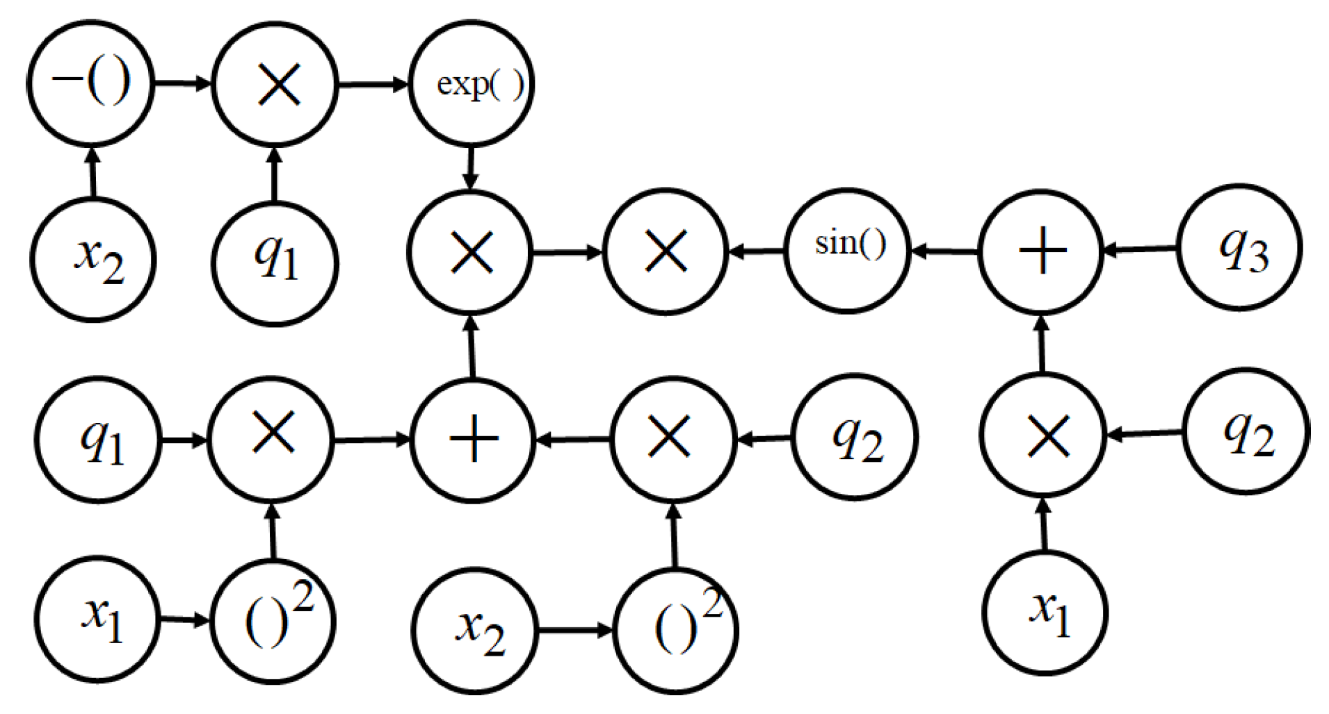
GP codes the mathematical expression in the form of computational tree.
Figure 1 shows the computational tree for the example mathematical expression (
30).
In the computer memory the mathematical expression is written in the form of an ordered multi-set of integer vectors with two components, the first component is the number of arguments of function, the second component is a function number.
The code of GP for the example is
Despite the popularity of the method, it has a computational weakness. The code of GP has different length for different mathematical expressions. In this regard, other methods considered below seem to us more attractive from a computational point of view.
4.2. The Network Operator
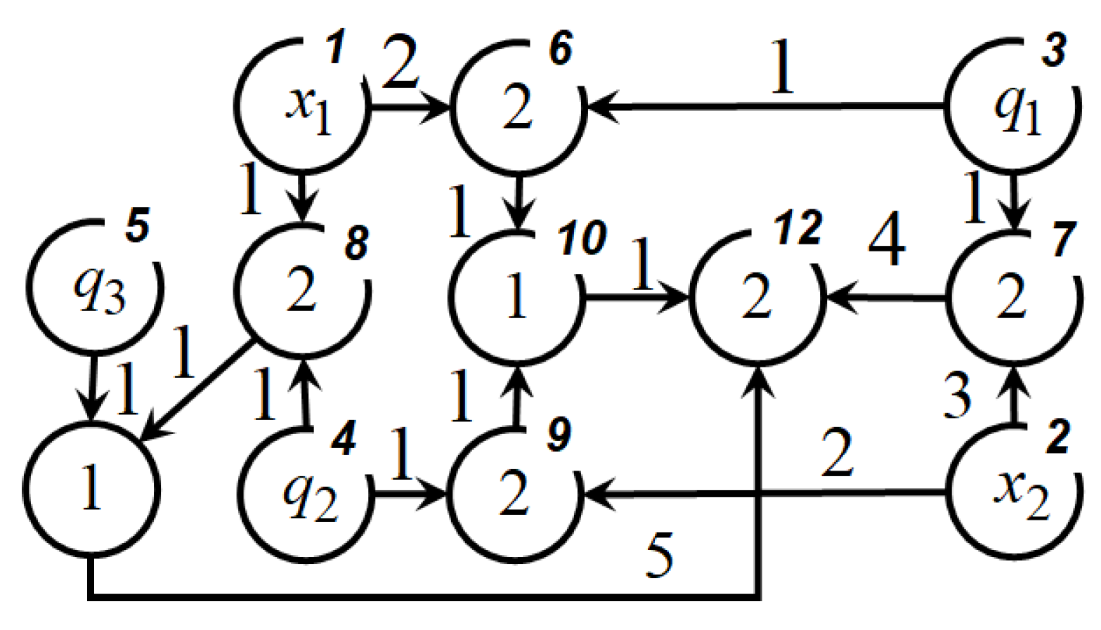
The network operator method (NOP) codes a mathematical expression in the form of oriented graph [
15]. Source-nodes correspond to arguments of the mathematical expression, other nodes correspond to functions of two arguments, and arcs correspond to functions with one argument.
The graph of NOP for the mathematical expression (
30) is presented in
Figure 2.
In the graph (
Figure 2), numbers near arcs are numbers of functions with one argument. Numbers inside nodes (except source nodes) are numbers of functions with two arguments. Numbers in upper parts of the nodes are the node numbers.
In the computer memory the NOP-code of the mathematical expression is presented in the form of an integer matrix. The NOP matrix of the mathematical expression (
30) is
In the matrix of NOP, each line corresponds to a node. Nonzero numbers in the main diagonal are numbers of functions with two arguments. Other numbers are numbers of functions with one argument.
4.3. Cartesian Genetic Programming
Cartesian genetic programming (CGP) encodes consecutive calls of elementary functions [
13]. To encode a call, the sets of elementary functions is united
For the example the following set of elementary functions is obtained
CGP encodes every call in the form of an integer vector. The first component of this code is a number of the element from the set (
36). Other components are numbers of elements from the set of arguments. As soon as the elementary function is calculated, the result is included into the set of arguments (
24) of the mathematical expression, therefore, after every calculation, the number of elements in the set of arguments is increased. A number of components of integer vector is equal to the largest number of arguments and plus one for function number.
To encode the example function (
30) three components are enough. The CGP code of the mathematical expression from the example has the following form.
4.4. Binary Complete Genetic Programming
The binary complete genetic programming (BCGP), unlike the genetic programming, has codes of the same length for different mathematical expressions [
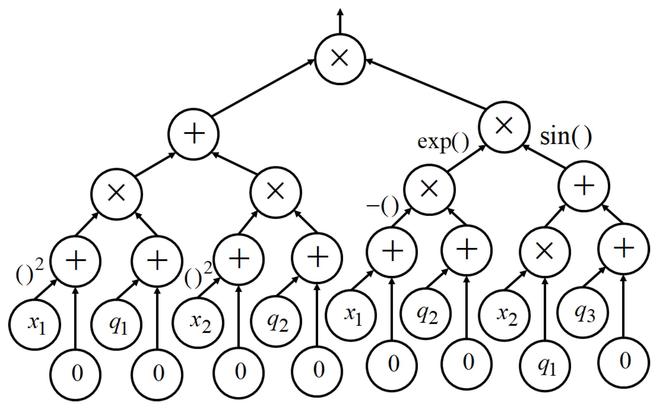
10]. The graph of BCGP for the example (
30) is presented in
Figure 3. In the BCGP graph, nodes correspond to functions with two arguments. Leaves correspond to arguments of the mathematical expression. Arcs correspond to functions with one argument. Each level has a certain number of elements equal to a power of two. In the code of BCGP extra functions are entered for obtaining complete binary tree.
In the computer memory, the BCGP code is presented in the form of an integer array with determined number of elements. The number of elements depends on the number of levels in the complete binary tree.
The BCGP code for the example is
The last level contains numbers of elements from the set of arguments (
31), where 6 is the number of unit element for the sum function
.
5. Computational Experiment
Now let us consider the solution of the control synthesis problem as MLC with the considered symbolic regression methods. Consider the problem of stabilization system synthesis for a mobile robot Khepera II [
27]. The mathematical model of the control object is
where
is a vector of state,
is a control vector.
The control has restrictions
The given set of initial conditions included 26 elements:
The terminal conditions were set as one point
It is necessary to find a control function in the form
where
are constant parameters,
, such that a robot from all 26 initial conditions (
42) got to terminal condition (
43) with minimal total time and high accuracy.
For solution of this problem, the network operator method, the Cartesian genetic programming, and the complete binary genetic programming were used with the principle of small variation of the basic solution.
Proportional controllers for each variable were used as a basic solution in all algorithms. The operations of addition and multiplication were used as binary operations, and a set of 28 smooth elementary functions was used as unary operations. The description of these functions can be found in the supplementary material to [
28].
The network operator found the following control law
where
, , .
The Cartesian genetic programming found the control law as (
45), where
, , , .
The complete binary genetic programming found the following solution (
45), where
, .
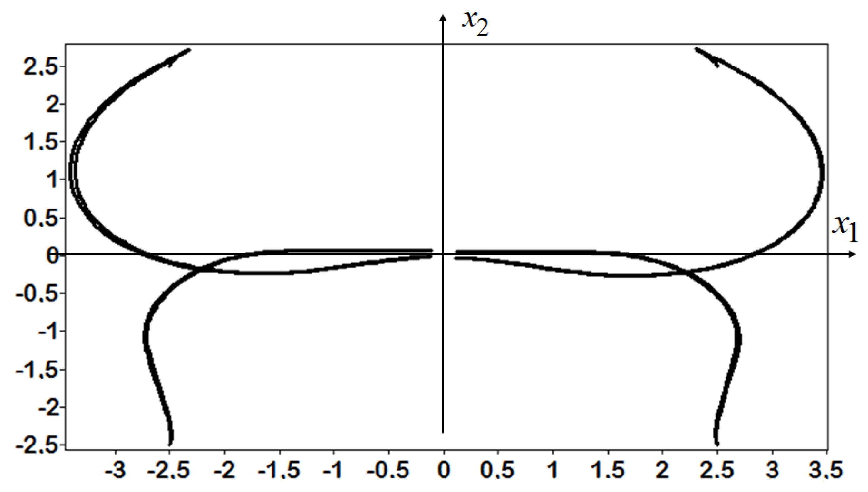
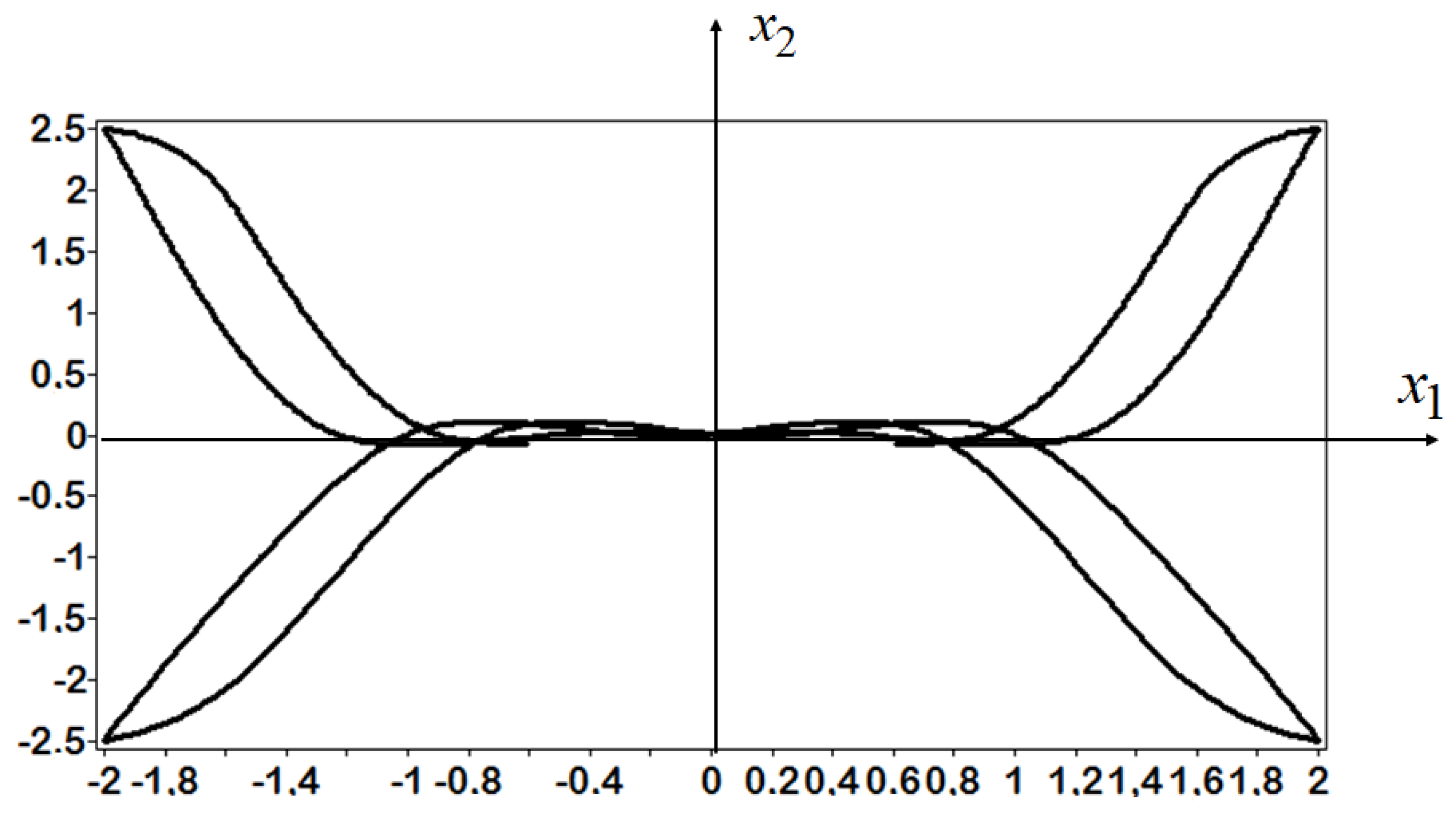
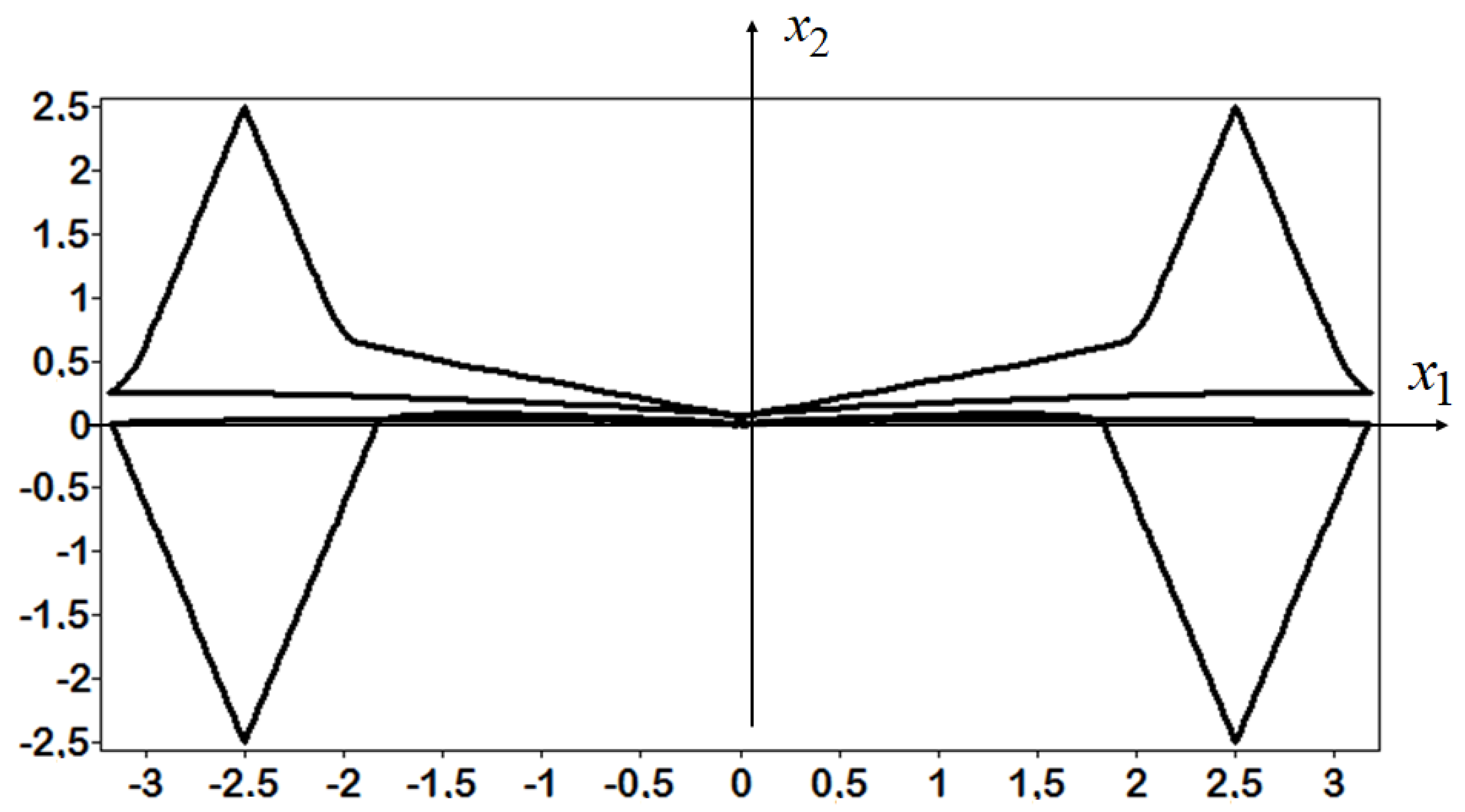
The trajectories of the robot moving from eight initial conditions (
52) to the terminal position (
43) are presented in
Figure 4,
Figure 5 and
Figure 6.
The goal of experiments was to show that computational symbolic regression methods allow to obtain a control function that, when substituted into the right-hand sides of a system of differential equations of the control object, makes this object stable. As a result, it was demonstrated that various symbolic regression methods can successfully solve this machine learning problem without laborious construction of a training set, basing only on the criterion for minimizing the quality functional.
6. Conclusions
The paper considered symbolic regression methods for machine learning control tasks. The theoretical formalization of MLC is proposed. The paper focused on the control synthesis problem as MLC. The scope of application of symbolic regression methods for supervised and unsupervised machine learning is discussed. The principle of small variations is considered to overcome the computational difficulties of symbolic regression methods associated with the complexity of the search space. Computational example of control synthesis for a mobile robot demonstrates the capabilities and prospects of such symbolic regression methods as network operator, Cartesian genetic programming and binary complete genetic programming as unsupervised machine learning control technique. Thus, the presented possibilities of various methods of symbolic regression in the field of machine learning control open up new perspectives in the field of control associated with the departure from manual and analytical search for solutions and the transition to machine search and machine learning control.
