Methods for Preventing Visual Attacks in Convolutional Neural Networks Based on Data Discard and Dimensionality Reduction

Abstract

The article is devoted to the study of convolutional neural network inference in the task of image processing under the influence of visual attacks. Attacks of four different types were considered: simple, involving the addition of white Gaussian noise, impulse action on one pixel of an image, and attacks that change brightness values within a rectangular area. MNIST and Kaggle dogs vs. cats datasets were chosen. Recognition characteristics were obtained for the accuracy, depending on the number of images subjected to attacks and the types of attacks used in the training. The study was based on well-known convolutional neural network architectures used in pattern recognition tasks, such as VGG-16 and Inception_v3. The dependencies of the recognition accuracy on the parameters of visual attacks were obtained. Original methods were proposed to prevent visual attacks. Such methods are based on the selection of “incomprehensible” classes for the recognizer, and their subsequent correction based on neural network inference with reduced image sizes. As a result of applying these methods, gains in the accuracy metric by a factor of 1.3 were obtained after iteration by discarding incomprehensible images, and reducing the amount of uncertainty by 4–5% after iteration by applying the integration of the results of image analyses in reduced dimensions.

1. Introduction

Today, computer vision systems are very important in many industries and fields. In [1], a brief overview of the application of computer vision algorithms in automation and robotics is provided. Technologies that use graphs in computer vision are now being used [2]. In [3] an analysis of combinations of image descriptors that are used was performed, which makes it possible to significantly improve the quality of image processing in relation to the task of analyzing images of industrial parts without textures. The main idea of this process is to use a support vector machine, which, for this narrow class, allowed more efficient processing than that of deep learning models.

Nevertheless, it is rightfully believed that a significant leap in the quality of computer vision systems occurred with the advent of deep learning methods [4]. With the growth of computational capabilities, the complexity of convolutional neural networks (CNNs) began to increase. One such breakthrough is considered to be the emergence of the AlexNet network [5], which significantly surpassed all previously known metrics in recognition tasks. The network successfully recognized images from the ImageNet database, where the input images were submitted in a size of 224 by 224 pixels, after which they were sequentially passed through paired convolution and pooling layers, providing feature extraction using convolutional kernels. The authors of [5] managed to achieve great success due to their use of drop out regularization, which, in 2012, had just begun to be used, and was described in detail in [6]. These architectures were further supplemented by next generation CNNs, such as VGG [7], Inception [8], ResNET [9], and Xception [10]. In [7], an architecture with 16–19 weight layers and a small convolution kernel (3 by 3) was proposed. The first version [8] of Inception was a little deeper; namely, it had 22 layers. However, in 2014, it became the state-of-the-art (SOTA) model in image recognition, since the authors managed to choose an architecture that was the most efficient at the time in terms of resource use. In [9], a network with 152 layers was considered, which made it possible to reduce the error rate on the ImageNet dataset to 3.57%. Further improvements [10] allowed the 123-layer network to extract nearly 23 million features from the image.

The development of algorithms for detecting objects in images has become a logical extension of the recognition task. The main idea is that it is possible to solve the recognition problem on a limited local area of an image. This is how the R-CNN network was suggested for detection and recognition by Ross Girshick [11]. R-CNN proposes an algorithm for the selection of regions or local areas in an image. However, the operation of such a network was rather slow, since it was necessary to perform convolution for each proposed region, most of which were unsuccessful, i.e., they did not contain objects. Moreover, they could partially enclose an object in the form of a bounding rectangle; it is important for the algorithm that the frame bounds the directly detected object, and not be a part of it. Then, the Fast R-CNN architecture was produced [12], where regions were formed directly on a feature map obtained as a result of convolution and pooling. This required reflecting these regions in the original image, and a regression model was applied to refine the bounding box coordinates. The next step in acceleration was the emergence of an algorithm in which the method of forming regions was improved; the Faster R-CNN algorithm [13]. In this architecture, a special neural network is trained, which more efficiently suggests regions for subsequent object detection. Finally, in 2017, the Mask R-CNN architecture appeared in the R-CNN family of architectures [14], which solves, in addition to detection and recognition tasks, segmentation and instance object segmentation tasks.

This analysis shows that, in recent years, there has been a movement away from the transition of classical algorithms for image processing, based on the mathematical description of random fields [15,16,17], to algorithms based on convolutional neural networks [18,19,20,21], especially under the conditions of growing computational capabilities. In [22], a model of a convolutional network is proposed, the functionality of which depends on time. It should be noted that the network is multichannel and capable of solving a wider range of tasks, which, according to the authors, makes it suitable for use in real life.

However, there are a number of problems inherent to the convolutional network approach. First, in a number of tasks, even for the implementation of direct network operation and not just its training, significant computing resources are required. In this case, one can either optimize the inference rate [23] or apply procedures for fine-tuning [24], quantization [25], and distillation [26] of networks. Secondly, there may be problems with the amount of data needed to ensure good accuracy in solving problems in real-world applications. To eliminate this drawback, data augmentation algorithms are actively used [27,28]. Finally, a problematic issue is the instability of neural networks and the lack of understanding of the processes of outputting network responses. Recently, artificial intelligence has begun to actively impose requirements for its explanatory ability [29]. Moreover, convolutional networks are largely susceptible to influence from various visual attacks [30], which, on unbalanced datasets [31], can lead to an extremely low quality recognition. Figure 1 shows an example of changing the feature map when one pixel is distorted.

The first line shows the convolutional and pooling processes for the original image. The second line shows the convolution and pooling process for an image in which one pixel was attacked. Analysis of the changes caused by this distortion in subsequent processing shows that 4% of the information is distorted in the original image, 18.75% in the feature map, and 50% at the output of the max pooling layer. It should be noted that there is a zero coefficient in the convolution kernel and that the dimensions of the kernel are small enough–(2 × 2).

Attacks can be targeted [32] if they change the prediction of the model in accordance with the desired result, and not targeted [33], such as noise in an image, which can randomly change a CNN prediction. The fight against both is difficult enough; for example, in [34], a method of teaching diversity was proposed to combat attacks. The goal of this method is to train the model more flexibly. However, in this case, it can be heavily over trained. In [35], use of a special loss function is proposed, which is determined by the difference between the model output for a not-attacked and an attacked image. However, its field of application is limited to filtering tasks, which can be successfully and efficiently solved using methods for reducing the dimensions of data [36]. Simultaneous dimensionality reduction and image noise removal is possible using singular value decomposition (SVD) [37].

It also should be noted that CNNs are only a part of image processing algorithms. In computer vision, the model-based approach [38,39] and structural system identification [40,41] are widely known. Model-based algorithms do not require resources and time for learning, and structural methods can be applied for analyses of complex structures in images, such as in structural engineering in aerospace, civil construction, mechanical systems, etc. Nevertheless, for processing for one referral, typical general images of handwritten numbers and animals, convolutional neural networks have proven themselves effective.

In this work, the simplest types of visual attacks are used, including additive white noise, point noise, and damage to the image area. To combat these attacks, an approach is proposed that is notable for its scientific novelty and allows to increase the efficiency and stability of CNNs using an ensemble of two models. The first model pre-learns to distinguish between affected (attacked) and unaffected (not attacked) images, thereby leaving only the answers with which the CNN is efficient. The second model, in turn, performs matrix SVD procedures for feature reduction and noise suppression. Then, for different dimensions, the recognition results are compared based on labels inherent only in undistorted images. As a result of the second network operation, the results of the first network are refined. Efficiency and stability are understood here as the ability of a network to (a) show a high percentage of the share of correct recognitions and (b) skip few visual attacks. In particular, it was possible to increase the accuracy of the metric by 30% and return about 5% of the distorted images, giving them the correct label. Comparisons are made with respect to the same networks where the proposed preprocessing methods were not applied.

2. Materials and Methods

Let us introduce the concept of a visual attack on CNNs and the types of attacks that will be considered in this article. If a distorted image is fed into the network input in a special way (according to the specified rules), then such a process will be called a visual attack. The distortion process itself is described by specified rules and can be implemented in different ways, forming different types of attacks. Within the framework of this article, the main attention is focused on the development of more universal methods of dealing with visual attacks; therefore, the types of attacks used in this task are not so important. For simplicity, the following types of attacks will be analyzed in the following sections.

(1) Distortion by white Gaussian noise with different variances.

We will assume that the brightness of an image at each point and color channel is described by the function $F(c,x,y)$, where $c$ (color) characterizes one of the three color channels in RGB; and $(x,y)$ is the spatial coordinates of the pixel in the specified chroma channel. If the brightness storage system is used in the uint8 data type, then the values can vary in the range of 0 (black corresponds to 0 in all channels) to 255 (white corresponds to 255 in all channels), then a change in noise should not lead to overshooting this range. To do this, it is possible to use a simple procedure for equalizing noisy images. The expression that allows to form a distorted noisy image can be written using Formula (1).

$$A_1(c,x,y)={[F(c,x,y)+N(0,\sigma )]}_{eq255},$$

(1)

where $N(0,{\sigma }_N^{})$ is random noise additive at any point, obeying the Gaussian distribution and characterized by zero mean and variance, ${\sigma }_N^2$; ${[\dots ]}_{eq255}$ is the brightness equalization procedure (for values from 0 to 255).

For the convenience of constructing comparative tables, this attack is named as “Attack No. 1”.

(2) One-pixel distortion

During this project’s implementation, the brightness of a randomly selected pixel was replaced by values close to the boundary values, i.e., for black pixels, the possible range of values is (0,1,2) and for white pixels it is (253,254,255). In this case, the same values are set for all color channels. As shown above (Figure 1), even a small change in the original image can lead to a strong modification of the feature vector used for recognition. The image model with a distortion of one pixel can be written as Formula (2).

$$A_2(c,x,y)=\{\begin{array}{c}F(c,x,y),\begin{array}{cc}if& (x,y)\ne (x_0,y_0),\end{array}\\ 0(255)+(-)j,\begin{array}{cc}if& (x,y)=(x_0,y_0),\end{array}\end{array}$$

(2)

where $j$ is random integer from (0; 3) interval.

Since changes are made within the range of 0–255, additional equalization of the distorted picture is not required.

For further convenience, we will call this attack “Attack No. 2”.

(3) Single color distortion of the image area

This type of attack is based on the idea of Attack No. 2, with the difference being that, instead of changing the brightness of one pixel, a procedure of maximizing or minimizing the brightness of a group of pixels located in a certain local neighborhood takes place. The attack implies that the brightness values inside this neighborhood will be the same for all pixels. In the simplest case, a rectangular area can be distorted. The model of such an attack can be written in accordance with Expression (3).

$$A_3(c,x,y)=\{\begin{array}{c}F(c,x,y),\begin{array}{cc}if& (x,y)\notin D_0,\end{array}\\ 0(255)+(-)j,\begin{array}{cc}if& (x,y)\in D_0,\end{array}\end{array}$$

(3)

where $D_0$ is a local area with a given distorted brightness.

Further in the text, we refer to this type of attack as “Attack No. 3”.

(4) Binary distortion of the image area

This type of attack develops the “Single color distortion” attack. Binary distortion refers to the replacement of pixels with two possible brightness values. In practice, in the case of this attack, it is necessary to change all pixels belonging to a region so that the probability of accepting “white” or “black” brightness is the same. The fulfillment of this condition is not difficult. A local area binarization procedure can be performed by generating a random number that obeys a uniform distribution and is in the range of (0; 1). Such a number with a 50% probability will be greater than 0.5, and, therefore, such a threshold will allow performing a close-to-equal pixel division. Extending Expression (3) to Formula (4) we get:

$$A_4(c,x,y)=\{\begin{array}{c}F(c,x,y),\begin{array}{cc}if& (x,y)\notin D_0,\end{array}\\ \begin{array}{l}0+j,\begin{array}{cc}if& (x,y)\in D_0,ran{d}_{(x,y)}<0.5\end{array},\\ 255-j,\begin{array}{cc}if& (x,y)\in D_0,ran{d}_{(x,y)}\ge 0.5,\end{array}\end{array}\end{array}$$

(4)

where $ran{d}_{(x,y)}$ is random real value from the range (0; 1) generated for a pixel with coordinates $(x,y)$, belonging to region $D_0$.

The attack leading to changes in the original image by Expression (4) will be referred to as “Attack No. 4”.

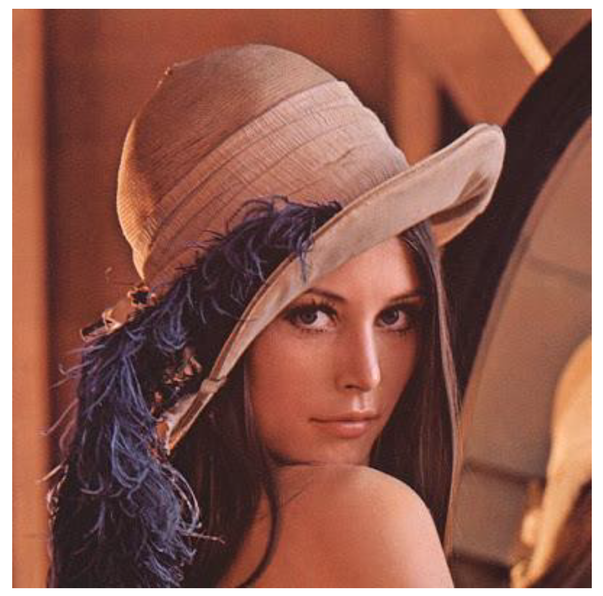
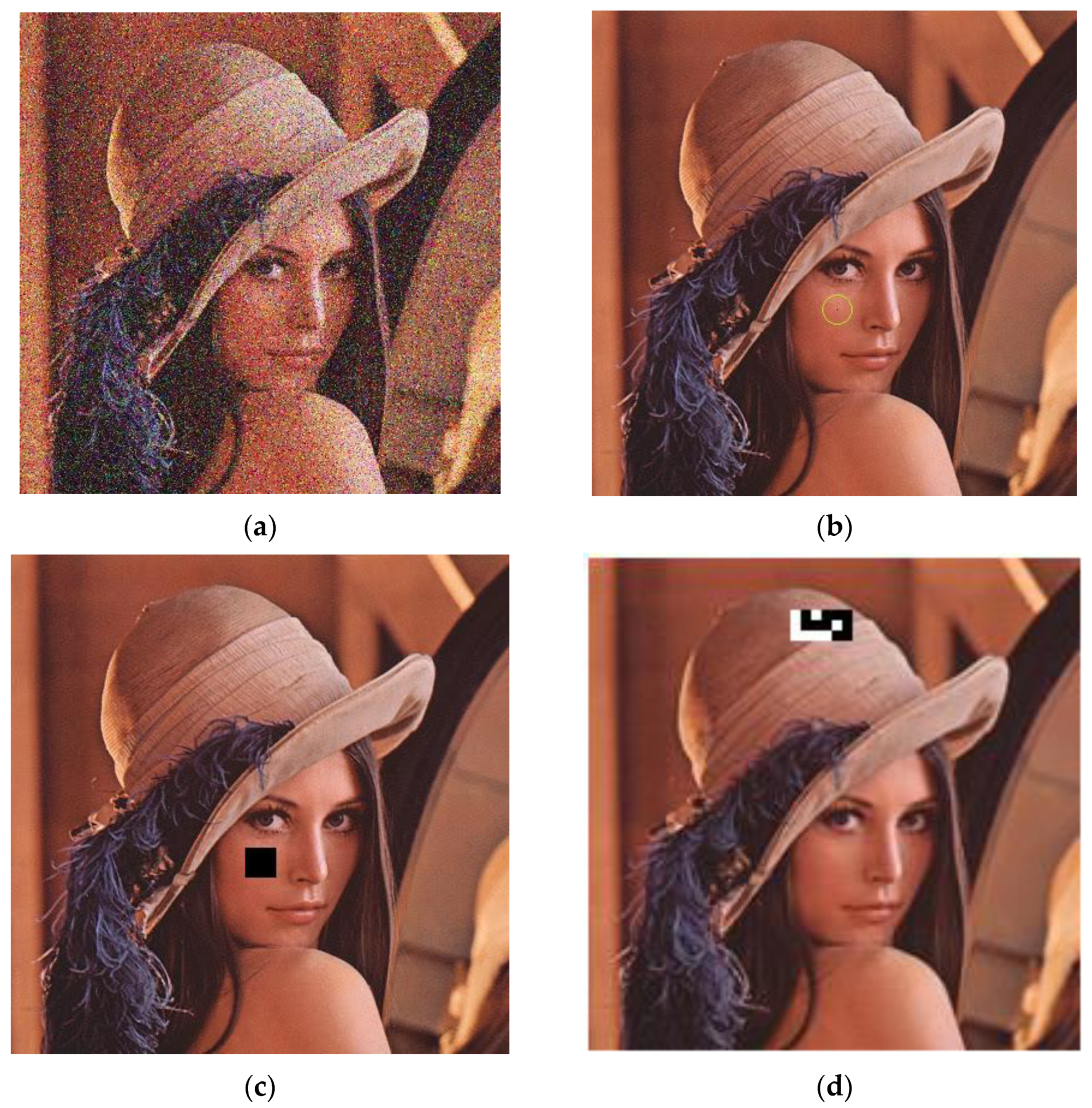
Using the Lena image as an example, which is widely used by specialists in the field of image processing and is available from the University of Southern California (USC SIPI) image database [42], we will show the results of the impact of the visual attacks described by Expressions (1)–(4). Figure 2 shows the original image. Figure 3 shows the original image subjected to the attacks. In other words, Figure 3a shows the superposition of Gaussian noise with a variance two times less than the signal variance. Figure 3b shows a distortion of one pixel, Figure 3c shows single color distortion of the image area, and Figure 3d shows binary distortion of the image area.

It should be noted that, in Figure 3b, the distorted pixel is located in the center of the additionally represented circle. It also should be noted that, for Figure 3d, the damage area is arbitrarily chosen, for simplicity as a rectangular shape and the black and white pixels are random.

In the task of recognition, color channels can often be neglected if color is not a priority feature for the objects being recognized. However, acceptable quality is usually also achieved with grayscale images. Thus, before applying the methods of dimensionality reduction, it is possible to reduce the original number of features (pixel brightness) by a factor of three times. Then, we turn to a two-dimensional representation of the image instead of a multidimensional one, such as $M\times N\times 3$, where $M$ is number of pixels in a column and $N$ is the number of pixels per row. Then, if we represent the image in the form of a matrix of dimensions, $M\times N$, using the SVD of matrices, one can then arrive at the dimension $\tilde{M}\times \tilde{N}$, where $\tilde{M}\le M$, $\tilde{N}\le N$. The SVD for a matrix $A$ has the following Formula (5):

$$A=UW{V}^T,$$

(5)

where $U$ is a rectangular matrix with the dimension $M\times N$; $W$ is diagonal matrix with $N\times N$ sizes, consisting of the singular values of the matrix, $A$; and $V^T$ is transposed matrix $V$ with dimensions $N\times N$.

Based on an analysis of the singularity of the matrix $A$ it is possible to evaluate its rank, range, and zero space. Decomposition (5) can also be used to reach the dimension $\tilde{M}\times \tilde{N}$, where $\tilde{M}\le M$, $\tilde{N}\le N$.

To determine the SVD, you must first introduce matrix $A$ into Formula (6).

$$A=PBS,$$

(6)

where $B$ is a bidiagonal matrix and $P$ and $S$ are matrices obtained by iterative application of the Householder transform [43]. QR decomposition [44] is sought at the second stage for bidiagonal matrix $B$. This must then provide the validation of Expression (7).

$$B=Q^{T}WQ,$$

(7)

where $W$ is the sought diagonal matrix from the SVD, $Q$ ($Q^T$) are matrices obtained through iterative zeroing of rows (columns) of matrix $B$ using Givens rotation [45].

Finally, substituting $B$ From (7) into (6), we can write the singular value decomposition (8) for matrix $A$.

$$A=P{Q}^{T}WQS,$$

(8)

where $U=P{Q}^T$, $V^T=QS$.

The resulting expansion will be used to reduce the dimension.

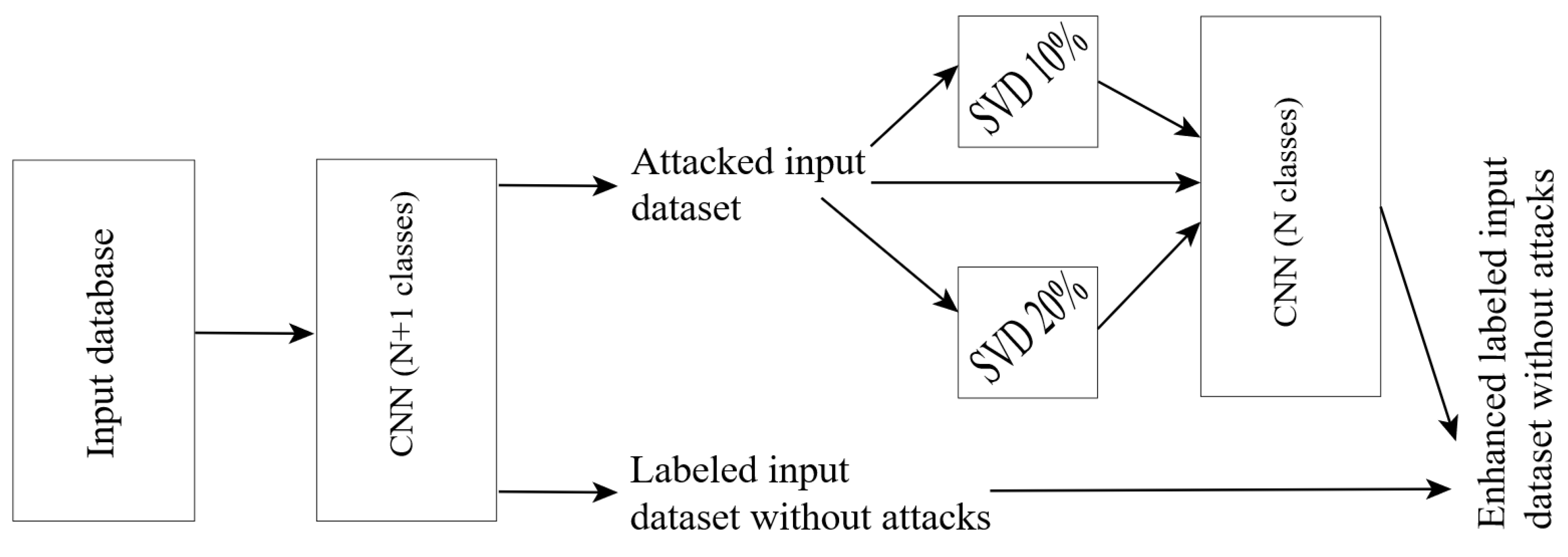
The idea of the proposed algorithm for preventing visual attacks is that you can first teach a network to distinguish distorted images and then discard them with the “attacked” label. This approach will potentially allow obtaining a large proportion of correct recognitions directly from the pre-filtered images. For the rejected images, alternate dimensionality reduction will be performed based on the SVD. The original rejected image and images reduced by 10% and 20% will be passed through a network that cannot distinguish between distorted images. If all 3 classifiers give the same answer, then such an image will be returned to the undistorted database with a corresponding label. Figure 4 shows a diagram of the described ensemble. Units SVD means SVD with different levels of feature reduction.

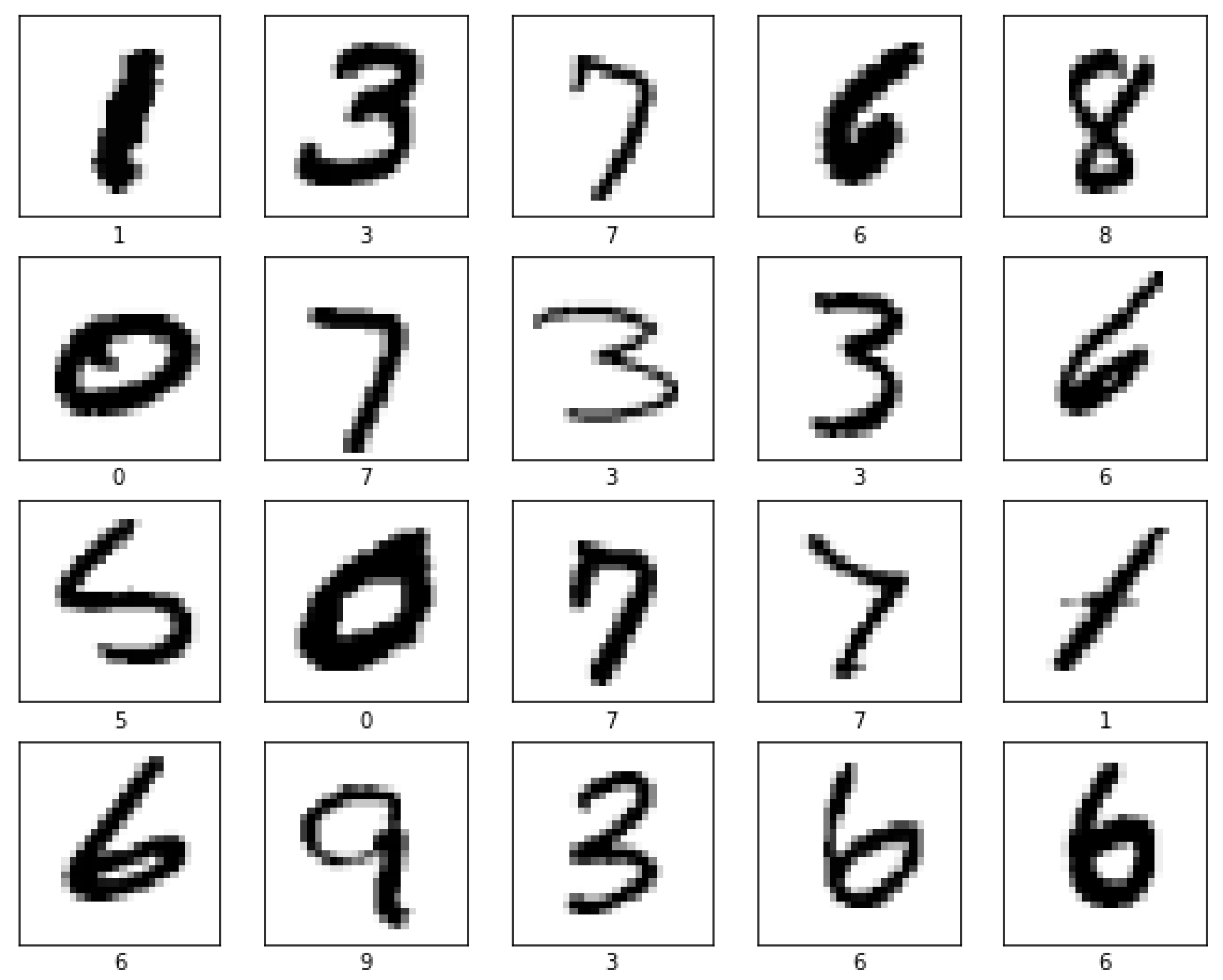
Note again that, for the scheme shown in Figure 4, the input images will be presented in grayscale. Since the analyses will be performed for datasets with an equal number of instances in each class, the use of additional metrics, such as precision and recall [46], is not required. We will only evaluate the probability of correct recognition in the dataset. This metrics is also known as accuracy. For this study, the MNIST dataset was first selected, namely MNIST.DIGITS, which contains 28 × 28-pixel images of handwritten digits. The MNIST database contains 60,000 images for training and 10,000 images for testing [47]. Half of the training and testing samples were from the NIST training set and the other half were from the NIST testing set [48]. Figure 5 shows examples of some images from the MNIST.DIGITS set.

Using the examples in Figure 5, it becomes obvious that the main task is recognition, since each image contains only one digit. Considering the size of the images, 28 × 28, the distortion of the rectangular area can only be carried out with side lengths of 2 and 3 pixels.

Using the specified MNIST database, we will prepare two separate datasets. In the first, all images will remain original (not attacked), and in the second, a number of images will be subjected to the attacks discussed previously. To analyze the effectiveness of the proposed algorithm, the following sets were obtained:

(1) MNIST-1 set. Consists of 60,000 training images without distortion, as well as 6000 images for a test sample without distortion, 1000 images of a test sample with distortions by Attack No. 1, 1000 images of a test sample with distortions by Attack No. 2, 1000 images of a test sample with distortions by Attack No. 3, and 1000 images of the test sample with distortions by Attack No. 4.

(2) MNIST-2 set. Consists of 52,000 training images without distortion, 2000 training images with distorted by Attack No. 1, 2.000 training images with distorted Attack No. 2, 2000 training images with distorted Attack No. 3, and 2000 training images with distorted Attack No. 4; the test sample is similar to that described earlier. Distortions are evenly distributed over images of all classes.

Since the MNIST dataset does not allow for a qualitative study of the dependencies of the recognition accuracy on the size of distorted regions and the noise level, the dogs vs. cats dataset from the Kaggle portal is also used [49].

This dataset contains labeled images of cats and dogs. At the same time, the training sample contains 12,500 images of cats and 12,500 images of dogs, and the test sample contains 12,500 unlabeled images. For the convenience of further accuracy calculations, the test sample was compiled by truncating the training sample. This dataset does not have fixed image sizes, so additional scaling procedures were applied. All images were reduced to 150 × 150 pixels just before being fed to the convolutional network. These sizes are 5 times the size of the MNIST images, so the size of the distortion regions ranged from 2 × 2 pixels to 15 × 15 pixels. 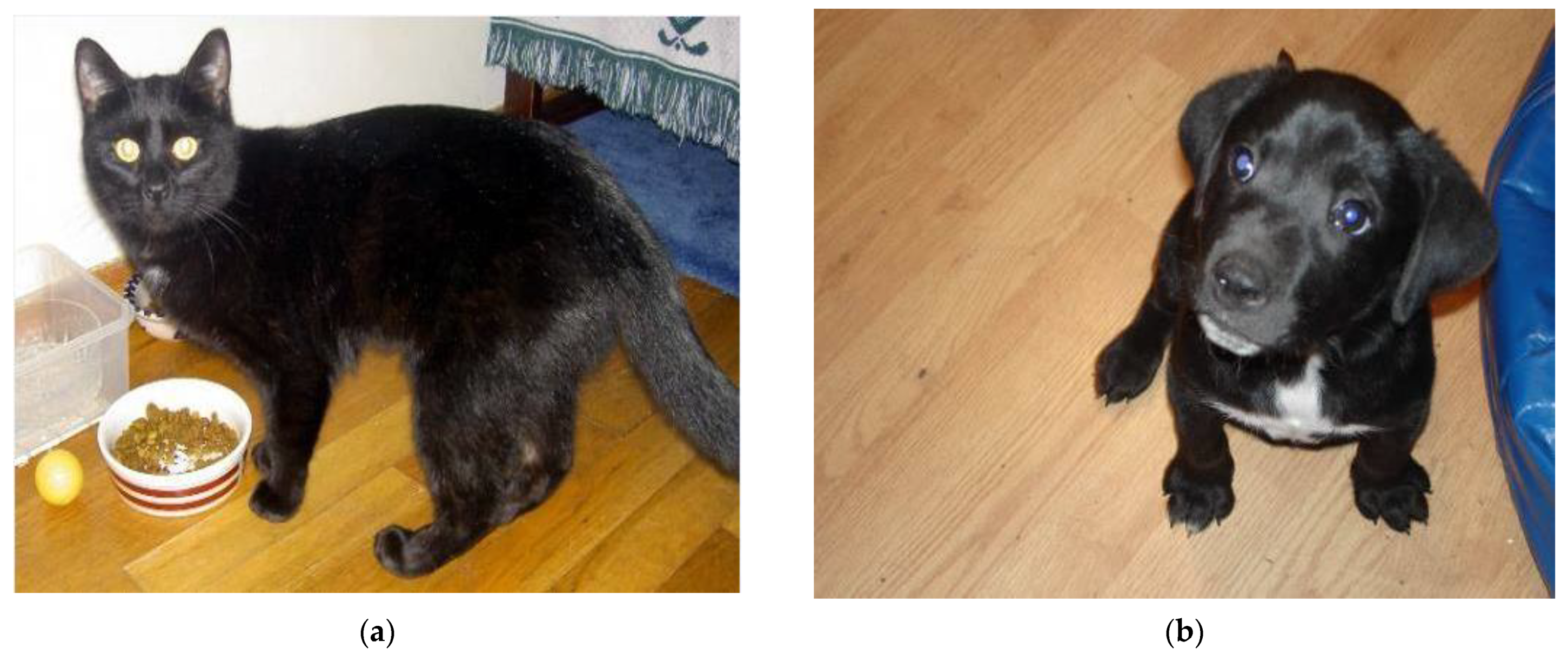Figure 6 shows examples of images with a cat (a) or a dog (b).

Note that, the presented in Figure 6 color images of arbitrary sizes were converted to grayscale images of specified sizes. Since there are only 2 classes in such a database, and only one class is represented in each image, provided that the classes are balanced, we define the accuracy metric as the main one. Furthermore, it becomes obvious that the images are presented in such a way that each of them belongs to only one of the two classes. To analyze the effectiveness of the proposed algorithm, the following sets were obtained from the dogs vs. cats data:

(1) DVC-1 set. Contains 18,000 distortion-free training images; 5000 images of the test sample without distortion, 500 images of the test sample with distortions by Attack No. 1, 500 images of the test sample with distortions by Attack No. 2, 500 images of the test sample with distortions by Attack No. 3, and 500 images of the test sample with distortions by Attack No. 4.

(2) DVC-2 set. Contains 15,600 training images without distortion, 600 training images with distorted by Attack No. 1, 600 training images with distorted by Attack No. 2, 600 training images with distorted by Attack No. 3, and 600 training images with distorted by Attack No. 4; the test sample is similar to that described earlier.

For both datasets, the signal-to-noise ratios are set in Attack No. 1 in the range of (0.2; 2).

The proposed algorithm was tested both on well-known CNN architectures and on a network with a full learning process. In total, during the recognition process, characteristics were obtained for the following three architectures:

(1) The VGG-16 network is a learning transfer-based architecture [50]. During the transfer, only the fully connected layer was trained to extract features that are important for the training data. Feature prefetching has always followed the VGG-16 architecture. The basic idea behind VGG architectures is to use more layers with smaller filters. In the VGG-16 version, the architecture consists of 16 layers. With small filters, you do not get many parameters, but you can handle them much more efficiently. Training is performed with a fully connected layer of 256 neurons. In the rest of the text, we will call this network “VGG-16”.

(2) The Inception-v3 network is a learning transfer-based architecture [51]. Learning takes place only for the fully connected layer, similar to the VGG-16 architecture. The main ideas of CNN Inception-v3 are as follows:

−

maximizing the flow of information in the network due to the careful balance between depth and width. Property maps are incremented before each pooling;

−

with increasing depth, the number of properties, or the width of the layer, also systematically increases;

−

the width of each layer is increased to increase the combination of properties before the next layer;

−

only 3 × 3 convolutions are used whenever possible. Considering 5 × 5 and 7 × 7 filters can be decomposed with multiple 3 × 3 convolutions.

Training is performed with a fully connected layer of 256 neurons. Further in the text we will call this network “Inception-v3”.

(3) The architecture of the simplest convolutional network has the following settings: 2 × 2 kernel and 5 hidden layers, with 16, 32, 64, 128 and 256 inputs, respectively. A fully connected layer also consists of 256 elements. Since 5 layers of convolution are used, hereinafter we will call this network “CNN-5”.

The next section discusses the obtained results.

3. Results

Since we managed to provide balanced datasets for the research, we restricted ourselves to analyzing only the accuracy metric, which actually reflects the proportion of correct recognitions. All subsequent results of measuring the proportion of correct recognitions, which are presented in this section, were obtained using a graphics computing device (NVIDIA GeForce GTX1060 3 GB GDDR5 1708 MHz video card), which made it possible to speed up the calculations in comparison with a CPU.

First, a study of the influence of Attacks No. 1 and No. 3 was carried out in order to determine the noise levels and the sizes of the distorted areas. Since the sizes of the images in the dogs vs. cats dataset provided a wider range of sizes for the distortion regions, only this dataset was used.

Table 1. Dependence of the proportion of correct recognitions on the signal-to-noise ratio (SNR).

Architecture	SNR = 0.2	SNR = 0.5	SNR = 1	SNR = 1.5	SNR = 2
VGG-16	81.38	83.16	84.32	89.65	91.37
Inception-v3	82.55	84.01	85.11	90.32	92.16
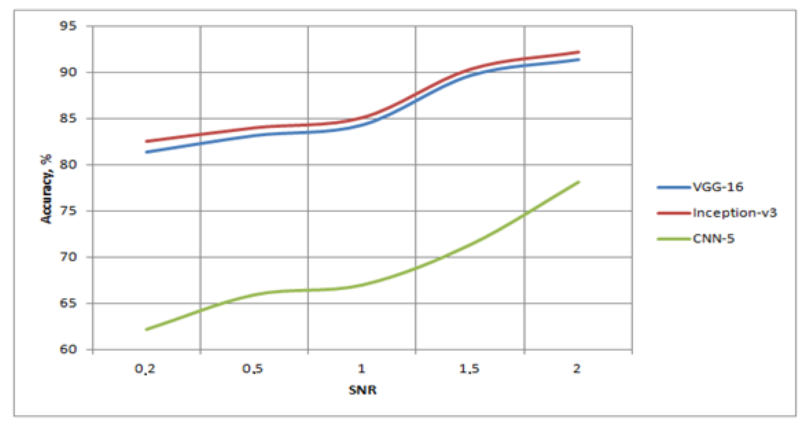
CNN-5	62.22	65.96	67.02	71.37	78.12

shows the characteristics of recognition when using only Attack No. 1 in the test set and only non-distorted images in the training set. The DVC-2 kit was selected for research. At the same time, different noise levels were set for Attack No. 1.

Due to our intentions to test the procedure using an extreme worst-case scenario, low SNR levels were also investigated. An analysis of the obtained results showed that at signal-to-noise values greater than one, the transfer learning algorithms approached the limit in recognition possibilities, and that the CNN-5 algorithm provided insufficient accuracy, even with limited values. A visualization of Table 1 is shown in Figure 7. From the graphs presented in Figure 7, it can be seen that, before reaching SNR = 100%, a slow increase in the accuracy of neural networks was observed, of the order of 3–5%. However, after the signal was further increased in relation to the noise, the increase in accuracy reached about 10–15%.

Table 2. Dependence of the proportion of correct recognitions on the size of the distorted area.

Architecture	${\mathit{S}}_{\mathit{c}}/{\mathit{S}}_{\mathit{i}}=0.0002$	${\mathit{S}}_{\mathit{c}}/{\mathit{S}}_{\mathit{i}}=0.0007$	${\mathit{S}}_{\mathit{c}}/{\mathit{S}}_{\mathit{i}}=0.0028$	${\mathit{S}}_{\mathit{c}}/{\mathit{S}}_{\mathit{i}}=0.0054$	${\mathit{S}}_{\mathit{c}}/{\mathit{S}}_{\mathit{i}}=0.01$
VGG-16	89.65	88.32	85.11	83.07	80.08
Inception-v3	89.98	89.02	86.49	84.22	80.65
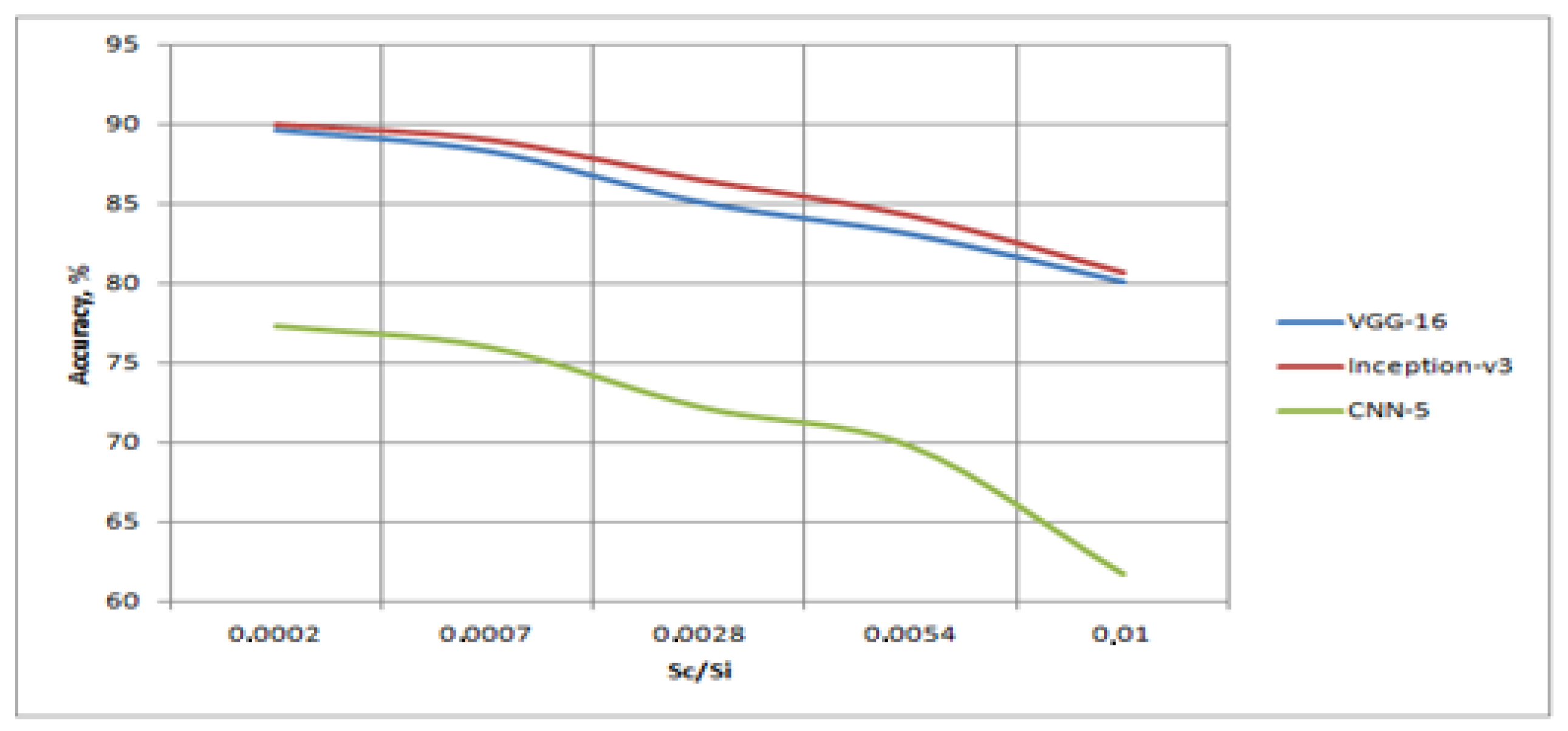
CNN-5	77.35	76.04	72.25	69.76	61.73

shows the characteristics of recognition when using only Attack No. 3 in the test set, and only non-distorted images in the training set. The DVC-2 set was selected for the research. At the same time, different sizes of distorted regions were set for Attack No. 3. However, since all the original images were 150 × 150 pixels in size, the dependence on the ratio of the area of the distorted area to the area of the image $S_c/S_i$ was investigated.

The analyses of the obtained results showed that at small distortion sizes, transfer learning algorithms are capable of demonstrating a high accuracy; however, a slight increase in the distortion area, up to 0.01 of the image area, led to a loss of about 10% in accuracy. At the same time, the CNN-5 algorithm was invariant to even smaller distortions, and, with an increase in the distortion area, its quality decreased sharply. A visualization of

Table 3. Percentage of correct MNIST.DIGITS image recognitions without prevention of visual attacks.

Architecture	No Attack	Attack No. 1	Attacks No. 1–2	Attacks No. 1–3	Attacks No. 1–4
VGG-16	72.83	79.64	82.35	88.65	94.67
Inception-v3	74.60	80.32	83.18	90.32	95.84
CNN-5	63.22	72.18	73.27	81.37	90.12

is shown in Figure 8.

Analyses made it possible to establish the values of the parameters of visual attacks based on the inflections of the graphs, i.e., for the SNR ratio, 1.1 was chosen, and for the area ratio, 0.001 was chosen. Further, all types of attacks and methods of dealing with them were investigated. For the curves in Figure 8, the situation was opposite to that in Figure 7. At first, the decrease in accuracy occurred very slowly, but after reaching the share of damage of 0.3%, especially for the CNN-5 network, a decrease in accuracy was observed.

Table 3 and

Table 4. Percentage of correct Kaggle.Dogs vs. Cats image recognitions without prevention of visual attacks.

Architecture	No Attack	Attack No. 1	Attacks No. 1–2	Attacks No. 1–3	Attacks No. 1–4
VGG-16	66.91	73.65	79.78	86.63	90.08
Inception-v3	70.32	78.54	82.16	88.82	92.32
CNN-5	60.10	65.55	68.94	73.45	80.64

present the results for the test sample, taking into account the classification into 10 (MNIST) and 2 (Dogs vs. Cats) classes. At the same time, images distorted by Attacks No. 1–4 were gradually added to the training set. Table 3 corresponds to the results for the MNIST handwritten number dataset, and Table 4 corresponds to the Kaggle dogs vs. cats dataset.

An analysis of the obtained results shows that the use of learning transfer is advisable, since the results of the VGG-16 and Inception-v3 networks were much better than those of a network trained from scratch, even in the absence of knowledge about possible attacks during training. In addition, the effect of adding distorted symbols to the training set was obvious. For example, for the Inception-v3 network, it was possible to increase the efficiency of correct recognition by 21% and 22% compared to the network, which was trained on the not-attacked images.

Table 5. Percentage of correct MNIST.DIGITS image recognitions with prevention of visual attacks.

Architecture	No Attack	Attack No. 1	Attacks No. 1–2	Attacks No. 1–3	Attacks No. 1–4
VGG-16	72.83	81.12	83.63	90.08	97.22
Inception-v3	74.60	82.54	84.90	92.64	98.55
CNN-5	63.22	73.07	75.25	83.37	91.09

and

Table 6. Percentage of correct Kaggle.Dogs vs. Cats image recognitions with prevention of visual attacks.

Architecture	No Attack	Attack No. 1	Attacks No. 1–2	Attacks No. 1–3	Attacks No. 1–4
VGG-16	66.91	75.12	81.80	87.92	91.74
Inception-v3	70.32	79.24	83.74	90.11	94.82
CNN-5	60.10	68.55	70.24	75.50	84.62

present the results from the test sample, taking into account classification into 11 (MNIST) and 3 (Kaggle) classes. Additional classes define distorted images that are not included in the calculation of the final accuracy metric. Thus, the share of correct recognitions was calculated only for images that did not fall into the added (distorted) class. Moreover, the data in the second columns of Table 5 and Table 6 were obtained when calculating the initial number of classes, i.e., 10 for MNIST.DIGITS and 2 for dogs vs. cats. This is due to the fact that, in the absence of distorted images in the training set, it is impossible to identify a new class. At the same time, images distorted by Attacks No. 1–4 in such a way that the distorted images constituted a new class were gradually included in the training set, similar to the experiments in Table 3 and Table 4. The accuracy of the network was finally recalculated only for images that the network classified as undistorted. Table 5 corresponds to the results for the MNIST dataset and Table 6 for the dogs vs. cats dataset.

Similar dependences noted for the results in Table 3 and Table 4 are preserved in Table 5 and Table 6. However, the main conclusion that can be drawn from the analysis of Table 5 and Table 6 is the conclusion about the effectiveness of the proposed method. Indeed, the use of attack prevention in post-processing allowed us to increase the proportion of correctly recognized images by 2–3%. Moreover, the best results in each case were provided by the Inception-v3 network, which provided 98.55% correct recognition for the MNIST.DIGITS image database and 94.82% for the Kaggle.Dogs vs. Cats image database.

However, this approach discarded about 25–30% of the images. Additional validation of these images with SVD can reduce this figure. Then you need to take into account the images revised by the architecture when calculating the recognition accuracy. The use of additional analysis with a reduction in dimensions by 10% and 20% allowed reducing the proportion of distorted images to 21–27%. At the same time, the accuracy characteristics change insignificantly, and in some cases even increased. The recalculated results are presented in

Table 7. Percentage of correct MNIST.DIGITS image recognition with prevention of visual attacks and reduction of dimension.

Architecture	No Attack	Attack No. 1	Attacks No. 1–2	Attacks No. 1–3	Attacks No. 1–4
VGG-16	72.07	81.16	83.33	90.02	96.58
Inception-v3	74.31	82.73	84.76	92.78	98.02
CNN-5	61.18	73.08	74.19	82.11	88.58

and

Table 8. Percentage of correct Kaggle.Dogs vs. Cats image recognition with prevention of visual attacks and reduction of dimension.

Architecture	No Attack	Attack No. 1	Attacks No. 1–2	Attacks No. 1–3	Attacks No. 1–4
VGG-16	66.94	72.11	80.95	87.96	91.76
Inception-v3	70.55	77.03	83.34	89.55	94.62
CNN-5	60.16	63.96	68.67	73.30	81.18

.

Analyses of the presented results shows that, on average, the accuracy characteristic for the studied datasets deteriorates after returning some rejected images. However, the recognition process is still robust. Thus, such algorithms can be used for enhanced output datasets with labels.

However, it is much more interesting to compare results against known and widely used architectures. Thus, it is possible to take our best network for each dataset; called Inception-v3 + Prevention + SVD, because using SVD allows the processing of more data. The comparison will be produced for data which were not rejected by our algorithm.

Table 9. Percentage of correct recognitions.

Architecture	Accuracy
MNIST
AlexNet	71.28
ResNet	73.32
Xception	75.61
Ours	98.02
Kaggle.Dogs vs. Cats
AlexNet	67.75
ResNet	71.90
Xception	71.82
Ours	94.62

presented the results for the MNIST and Kaggle.Dogs vs. Cats datasets. It should be noted that other architectures were learning on not-attacked images.

From Table 9, it can be seen that preventing attacks by using augmentations in training datasets shows great results in comparison to attempting to process images using neural networks which were trained only on clear data.

It was also interesting to test more complex types of attacks. The non-uniform noise generated in non-overlapping windows of different sizes and having different white Gaussian noises parameters was used.

Table 10. Non-uniform attack processing.

Dataset	3 × 3	5 × 5	7 × 7	10 × 10	15 × 15
MNIST	89.96	91.90	92.95	94.52	97.71
Dogs vs. Cats	85.15	85.73	86.88	89.12	91.10

presents the results for our best architectures and different window sizes. The noise expectation varies from −1 to +2 and noise variance lies in range from 0.1 to 2.5. The Gaussian noise model was randomly selected for each window. The average accuracy was calculated in 30 experiments.

From Table 10, it can be seen that a non-uniform noise decrease resulted for our solution. However, for big sizes of non-overlapping windows, it is possible to achieve results that are closest to the best ones for uniform noise. Results for MNIST are better because the images in the dataset were smaller.

4. Discussion

The article gave a brief overview of computer vision problems that are currently being solved using convolutional neural networks. Such networks are highly sensitive to various kinds of influences. In the work, simulating four types of influences were proposed: Gaussian noise, distortion at a point, distortion in an area with one color, and distortion in an area with two colors. For such attacks, studies were carried out on the dependence of the recognition accuracy on the noise level and the size of the distorted regions. It was found that upon reaching the signal-to-noise ratio of 1.1, the processing quality greatly increased (by 4–5%). In addition, when the relative area of distortions in an image was equal to 0.001, there as a sharp drop in the accuracy metric (by 3%). A procedure for filtering images based on training the network for known types of attacks was proposed, which made it possible to increase the average recognition accuracy by 20–25%. In order to reduce the number of rejected images, using a convolutional network block and a singular value decomposition block was proposed. The use of these blocks allowed, on average, to return about 4% of the rejected images to the output of the neural network. Transfer training using dogs vs. cats and MNIST datasets, using the Inception-v3 network, provided the best results among the considered architectures. Non-uniform noise decreased the quality of the model by 7–8%.

It should also be noted that the proposed algorithm is invariant with respect to neural network architectures. Augmentation with distorted images and training for new classes can be done using other architectures. The dimensionality reduction method, based on singular value decomposition of matrices, also implies only preprocessing data before feeding them to the input of a neural network. In particular, the implementation of such an algorithm makes it possible to increase the proportion of correct recognitions, based on the AlexNet network, by 16% and the return of up to 8% of distorted images. Further research can be aimed at improving the algorithm and using the ensemble based on ResNet, GoogleNet, and Xception architectures.

In the future, it will be necessary to improve the image return unit, but with the preservation of a high recognition accuracy. In addition, the results obtained also allow to conclude that an alternative approach to combat visual attacks without preprocessing can be augmentation of the training set using images distorted by various attacks. Perhaps the development of data augmentation algorithms that differ from standard methods will also improve the quality in the fight against visual attacks.