Abstract
In recent studies, self-supervised learning methods have been explored for monocular depth estimation. They minimize the reconstruction loss of images instead of depth information as a supervised signal. However, existing methods usually assume that the corresponding points in different views should have the same color, which leads to unreliable unsupervised signals and ultimately damages the reconstruction loss during the training. Meanwhile, in the low texture region, it is unable to predict the disparity value of pixels correctly because of the small number of extracted features. To solve the above issues, we propose a network—PDANet—that integrates perceptual consistency and data augmentation consistency, which are more reliable unsupervised signals, into a regular unsupervised depth estimation model. Specifically, we apply a reliable data augmentation mechanism to minimize the loss of the disparity map generated by the original image and the augmented image, respectively, which will enhance the robustness of the image in the prediction of color fluctuation. At the same time, we aggregate the features of different layers extracted by a pre-trained VGG16 network to explore the higher-level perceptual differences between the input image and the generated one. Ablation studies demonstrate the effectiveness of each components, and PDANet shows high-quality depth estimation results on the KITTI benchmark, which optimizes the state-of-the-art method from 0.114 to 0.084, measured by absolute relative error for depth estimation.
1. Introduction
Estimating depth from a single image is a significant computer vision task in enabling computers to comprehend real scenes. It has been widely applied in AR (augmented reality) [1], robotics navigation [2], and self-driving cars [3] for generating high-quality depth from color instead of using expensive LiDAR sensors. Although the monocular camera is cheap and light weight, the depth estimation task is still challenging for the traditional SfM/SLAM algorithm [4].
In the deep learning method of monocular depth estimation, it can be coarsely classified into two categories, supervised and self-supervised learning. For the supervised learning task, the original view to be estimated and its ground-truth depth data are both the input of the neural network [5]. The depth map is obtained by expensive LiDAR sensors [6], which is sparse compared with the original image on the pixel level. In the case of poor ambient light, the capability of LiDAR will be greatly affected. Therefore, the generalization ability of the prediction network trained by the ground truth depth map obtained by the LiDAR sensor is insufficient. When the trained model is applied to a new camera or to predict the depth of a new scene, the reliability of the prediction will be greatly reduced. Meanwhile, obtaining significant ground-truth depth data for the dataset is challenging. However, unsupervised learning methods utilize geometric constraints of stereo images as the only source of supervision, i.e., unsupervised learning takes the image obtained by a monocular camera as input and uses view synthesis to supervise the training network. This method is simpler than supervised learning and has a stronger generalization ability between different cameras and different scenes.
However, self-supervised methods still do not perform as well as supervised methods on the standard benchmarks. The reason lies in the weak supervision of the photometric consistency, which refers to the pixel-level difference between the image from a perspective and the reconstructed image generated by another perspective. Most of the previous unsupervised monocular depth estimation methods rely on the color constancy hypothesis, which assumes that if the original image and the reconstructed image are identical at corresponding pixels, then they should have the same RGB values at each other’s positions. However, in reality, as Figure 1 shows, many factors will cause color fluctuation, which may affect the color distribution. For example, the light intensity, noise and the reflection of light, etc., are different in two different views. Therefore, the unsupervised loss we use is easily affected by these common factors that interfere with the color. When the reconstructed image is generated from another image disturbed by the above factors, the losses incurred in the undisturbed areas are inaccurate, so that causing unreliable results when generating a depth map. The problem caused by color constancy hypothesis is referred to as the color fluctuation problem.
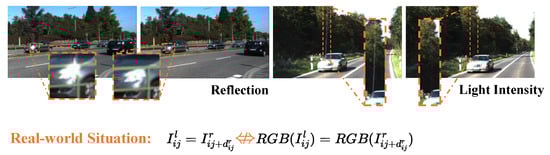
Figure 1.
Illustration of the color constancy hypothesis problem in previous self-supervised depth estimation task, where and represent the left and right view, represents the disparity map of the right view, represents the coordinates on an image, and RGB represents the RGB value on each pixel.
At the same time, the low texture problem also affects the depth estimation. In the low texture region of the two images, if the feature information is ambiguous, then the disparity map generated by the model may not be accurate. For example, when calculating the photometric loss in those regions, the loss values could be very small for the model to represent, but in fact, the two areas may not be the same.
To solve the above problems, we propose a novel self-supervised depth estimation network—PDANet, which contains two extra unsupervised signals: (1) the perceptual consistency uses the loss in the high-order semantics level rather than the pixel level, which brings abstract matching clues for the model to match the low texture and color fluctuation region. (2) The data augmentation consistency effectively enhances the robustness of the image to color fluctuation caused by illumination and other factors instead of applying color constancy hypothesis.
For the perceptual consistency, we use the outputs of several layers of the pre-trained VGG16 model to extract the abstract semantic information of the image and utilize the pyramid feature aggregation method to aggregate high-order and low-order features. Model training is supervised by minimizing the perceptual consistency loss between the generated image and the original image.
For the data augmentation consistency, we compare the unprocessed areas of two disparity maps, which are obtained by feeding the original image and the image after data augmentation on some areas into the network.
Table 1 shows the comparison between the above approaches and PDANet in terms of data acquisition, generalization ability, limitations, and prediction effect.

Table 1.
Comparison of different approaches.
An example result from our algorithm is illustrated in Figure 2. Specifically, our contributions are as follows:
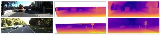
Figure 2.
Examples of PDANet’s results on KITTI2015 [6]. From left to right: input images, ground truth disparity maps, and results of PDANet.
- Based on the baseline monocular depth estimation network, we integrate data augmentation consistency and perceptual consistency as supervised signals to overcome the color constancy hypothesis and image gradient disappearance in low-texture regions for previous work.
- We propose a new unsupervised loss based on perceptual consistency to excavate the deep semantic similarity before and after image reconstruction so that the model still obtains genuine image differences in low texture and color fluctuation regions.
- We also innovatively propose a heavy data augmentation consistency to solve the color fluctuation problem and greatly enhance the generalization of the model.
2. Related Work
2.1. Supervised Depth Estimation
Since the ground truth is used as the supervising signal for the network in the supervised approaches, the deep network directly learns the mapping between the RGB map and the depth map. Eigen et al. [5] first use CNNs for the monocular depth estimation, the architecture consists of two components: coarse-scale networks to extract global information, and fine-scale networks to refine local information. Based on [5], they propose a unified multiscale network for three tasks: depth estimation, semantic segmentation, and normal vector estimation [7]. Laina et al. [8] propose a fully convolutional network, using residual networks to extract global information and designing residual up-sampling blocks to improve the quality of depth estimations.
Many methods have converted depth estimation to a classification problem. Cao et al. [9] discretize continuous depth values into several bins and use a CNN to classify them. Fu et al. [10] propose a spacing-increasing discretization strategy to discretize the depth, reconstructing deep network learning as an ordered regression problem to prevent over-strengthened loss.
Supervised methods require annotated datasets, while the acquisition of these datasets are costly. To alleviate the burden of the annotation task, weakly supervised methods in the form of supervised appearance matching terms [11], parse ordinal depths [12], and known object sizes [13] have been proposed. Since research on these tasks have reached a bottleneck, self-supervised monocular depth estimation has been explored in recent studies.
2.2. Self-Supervised Depth Estimation
The self-supervised approach is under photometric and geometric constraints instead of costly depth values. Many methods are developed in a supervised manner, either using stereo pairs or exploiting monocular sequences. Here, we concentrate on research related to self-supervised depth estimation based on stereo pairs.
Garg et al. [14] first present self-supervised depth estimation by converting the depth estimation problem into a left–right view stereo matching problem with photometric loss. Godard et al. [15] extend reconstruction constraints by disparity smoothness loss and left–right depth consistency loss. Tosi et al. [16] introduce a traditional depth estimation method, which generates proxy labels as supervised signals in the form of reverse Huber loss, image reconstruction loss, etc. Wong et al. [17] propose a new objective function to illuminate the bilateral cyclic relationship between the left and right disparity and introduce an adaptive regularization scheme to deal with the co-visible and occluded regions in stereo pairs.
To optimize the quality of depth estimation, various approaches have been developed, such as generating virtual three-eye views from stereo pairs [18], utilizing the adversarial learning framework [19,20], and designing a context-aware network [21].
3. Method
Here, we describe our PDANet for monocular depth estimation in detail. The PDANet is designed to require only a left view as input and output a disparity map , which is used to estimate depth on each pixel from the input image. As shown in Figure 3, the PDANet consists of three components: data augmentation consistency, photometric consistency, and perceptual consistency. It adopts the monocular depth estimation (Monodepth) model proposed by Godard et al. [13] as the baseline. The architecture is designed to enforce the depth estimation and robustness on low texture and color fluctuation areas. Moreover, it preserves spatial structures as much as possible.
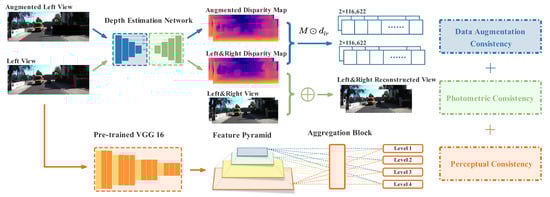
Figure 3.
Illustration of the overall architecture of PDANet, which consists of three components: data augmentation consistency, photometric consistency, and perceptual consistency.
3.1. Backbone of Depth Estimation
Most of the existing training methods are supervised learning methods. By comparing the real depth map with the predicted depth map, a loss is generated to reverse the prediction network and converge the model. However, due to different scenarios, it is challenging to obtain quantitative ground-truth depth data. However, Godard et al. [15] propose the Monodepth, which is a CNN-based model to calculate the disparity value of each pixel, a depth D is calculated by predicted disparity map d, as shown in Equation (1).
where f represents focal length of binocular cameras, and T represents the baseline distance.
The model applies the reconstruction loss, the disparity smoothness loss, and the left–right disparity loss as unsupervised signals to replace the ground-truth depth data. This model produces state-of-the-art results and even outperforms some supervised methods. Hence, we used Monodepth [15] as the basis of our depth estimation work. Next, we introduce the above-mentioned losses of photometric consistency.
3.1.1. Reconstruction Loss
Similar to [15], we input two images at the training time; the purpose is to generate the disparity map of the left image and calculate its corresponding depth map, the right view is the same. As shown in Equation (2) , is the loss before and after image reconstruction, is the original input image, is the image generated by the network, is set to , which is used to balance two weights. structural similarity (SSIM) and L1 are combined to generate to ensure that the reconstructed image is consistent with the original input image in the spatial domain.
3.1.2. Disparity Smoothness Loss
As discontinuities often occur at image gradients [15], is a smooth term on the disparity maps in Equation (3), which ensures the disparity maps are locally smooth. Here ∇ is a differential operator that computes the gradients of the disparity map and the input image. d represents the disparity map generated from the left view, and i, j are used to locate the coordinate of an image.
3.1.3. Left–Right (LR) Consistency Loss
To generate more accurate disparity maps, our network predicts both left and right disparity maps, while only receiving input as the left view to the CNNs part. To ensure the coherence, L1 left–right disparity penalty is applied to minimize the different between the left disparity map and the projected map. Equation (4) shows the LR consistency where or represents the left or right disparity map generated from the left view.
3.2. Perceptual Consistency
In previous self-supervised depth estimation networks such as Monodepth, the reconstruction work is supervised by minimizing the difference between the input image and its reconstruction image on a pixel level. However, in the low texture and color fluctuation areas, the ignorance of high-level semantic information affects the photometric consistency.
For the low-texture areas, we present the reasons in detail by calculating the gradient through the reconstruction loss [22]. Assuming that is the direct loss of the original image and the generated image at the pixel level, the gradient of on is calculated as follows:
The gradient of reconstruction loss mainly depends on the . In the low texture region, the gradient is close to zero so that the value of the entire equation closes to zero, resulting in the disappearance of the image gradient. However, high-level semantic features such as contours in the low-texture regions enhance the feature representation, greatly increase the image gradient, and improve the prediction capability of the model.
As for the color fluctuation regions, it is unreliable to use RGB values to evaluate the image reconstruction effect; however, the semantic features such as shapes and sizes of the objects in this region will not be affected by external factors; therefore, using high-level semantic features to evaluate the effect of image reconstruction will produce more reliable results.
Therefore, the perceptual loss is utilized to solve the above problems by ensuring multi-scale feature consistency. In this section, we describe our approaches, including feature extraction, feature aggregation, and computation of perceptual loss.
3.2.1. Feature Extraction
The perceptual loss aims at calculating multi-scale image losses at the semantic level. The pre-trained VGG16 is capable of feature extraction, e.g., some CNN layers of VGG16 are exploited to evaluate semantic differences between images in the field of style transformation and single-image super-resolution issue [23], etc. To evaluate the feature-wise differences in the reconstruction work, we apply a pre-trained VGG16 to extract feature representations. The backpropagation is not necessary for the feature extraction to work.
As shown in Figure 4, the output of VGG16 is a feature pyramid, which consists of four scale features obtained by convolution layer 2, 4, 7, and 9 of VGG16. Each layer is followed by an activation function ReLU. represents the feature maps extracted at level l for feature pyramid).
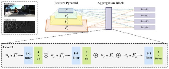
Figure 4.
Visualization of a feature fusion sample result and a brief illustration of feature aggregation. For each level, each layer of the original feature pyramid is resized to specific size and the number of channels and fused with specific weights.
3.2.2. Feature Aggregation
Multi-scale feature maps generated by VGG16 are used to excavate perceptual differences. Meanwhile, to refine our loss functions, we draw inspiration from recent works that aggregate features [24,25] to weave context information from multiple scales. At each new level, the aggregation block is constructed to fuse feature maps at all the levels in the pyramid. In Figure 4, the three steps of feature aggregation are exhibited: feature resizing, 1 × 1 filter, and feature aggregation.
Here, the convolution filter is utilized to modify the number of channels of to that of . For level l, we resize the feature maps at the other level to the same size as that of . Feature maps at four levels in the feature pyramids have different shapes, so we apply the up-sampling and down-sampling strategies to modify the shape at each level, e.g., at level 3, and need to be upsampled by transposed convolution and needs to be downsampled by a convolution layer with a stride of
To achieve better fusion for feature maps of the different receptive fields, we assign different weights to create stronger representative feature maps instead of using the sum of pixel wise.
The adjustment in weight parameters represents the contribution of feature fusion. Here, set and , for , , and are suppressed, and is enhanced by feature aggregation.
3.2.3. Perceptual Loss
At last, the multi-scale feature maps are generated by the VGG16 and the aggregation block, which contain contextual information from low-level to high-level representation, so we propose the perceptual loss based on to integrate self-supervision constraint to depth estimations.
Finally, the perceptual loss is measured by calculating loss between generated by the input left image I and generated by the reconstruction.
3.3. Data Augmentation Consistency
Some works [26,27] in contrastive learning show the benefits of data augmentation in self-supervised learning. The purpose is that data augmentation creates challenging samples, which interfere with the reliability of unsupervised learning losses and provide robustness towards different inputs. However, data augmentation is rarely used in unsupervised methods because it brings natural color interference to the original image. Therefore, we conduct the unsupervised learning by comparing the original data with the augmented sample output, rather than optimizing the original objective of view synthesis.
Assuming that a random vector is used to parameterize any data augmentation operation to the input image I, so an image is generated after operates on the original image I. As Equation (8) shows, the disparity map obtained by inputting an original image I generated by the disparity estimation network is Relatively, the disparity map obtained by inputting an augmented image through network prediction is We compare the disparity maps obtained before and after data augmentation through L1. Under the real-world situations, if we exclude the augmentation part of the two images, the remaining part of the disparity map generated by the two images should be the same. The disparity prediction is not interfered with by the changes of other pixels, which indicates that the prediction model generated in this case is robust. Therefore, the data augmentation consistency is guaranteed by minimizing the difference between d and is a three-dimensional matrix containing only a true or false value, which represents the unoccluded mask generated by augmentation operation . ⊙ is an operation used to obtain unprocessed parts in two images. The epipolar constraints between views confine us not to change the spatial location of pixels.
3.3.1. Random Masking
To simulate the possible occlusion problem in two images, we randomly add a binary mask to some areas of the original image to block these areas and project these masks to the corresponding positions of the right image. Assuming that the unoccluded regions are not affected by the occluded area when predicting the depth, we compare the unoccluded area of the original sample and the data augmentation sample to generate a loss that affects the model prediction. The random masking operation is presented by .
3.3.2. Gamma Correction
Gamma correction is a nonlinear operation to change the light intensity of the image. In this way, we strengthen the robustness of the interference caused by different scenes of light, so that the model adapts to the interference under different ambient light. The gamma correction operation is in form of .
3.3.3. Color Jitter and Blur
Many transformations on the image bring color interference to the image, such as color jitter, random blur, and so on. Owing to the color fluctuation, the loss generated by the regular training method based on color constancy may generate inaccurate results. Therefore, our method creates difficult scenes to strengthen the robustness of the model for color fluctuation problem under unsupervised training. The color jitter and blur operation is . Therefore, the final data augmentation transformation is combined by the above-mentioned three augmentations:
where ∘ represents function composition.
3.4. Overall Architecture and Loss
Above all, we use the additional perceptual consistency and data augmentation consistency as unsupervised signals on the baseline structure to solve the color constancy hypothesis problems mentioned above and enforce robust prediction towards low-texture regions. Hence, the final loss is defined as follows:
where the weights are set as: , . To have the same smoothness at each scale, r is used to rescale the disparity smoothing term . Thus , where r is the downsampling factor of this layer relative to the input image.
4. Results
Comprehensive experiments were conducted to evaluate our PDANet model. Firstly, we describe the experimental process and parameter settings of the baseline monocular depth estimation model using a single image as input. Secondly, the superior performance of the model on low texture and color fluctuation regions are presented by comparing our PDANet with the existing supervised and unsupervised models. Meanwhile, to demonstrate the effectiveness of each part of PDANet, we perform an ablation experiment by evaluating the performance of the Monodepth with and without perceptual consistency or data augmentation consistency.
4.1. Implementation Details
Our PDANet was implemented in PyTorch with about 31 million parameters and trained on a Titan RTX. The parameter setting and the split of dataset were the same as [15]. We trained the model for 30 epochs using the Adam optimizer; the batch size was set to 8. The initial learning rate was set to , which keeps constant for the first 10 epochs, then halved every 10 epochs until the end. Initially, we tested the reverse transmission of data augmentation loss separately; the model takes a single image as an input using the reconstruction loss as supervised signal, then serially uses another augmented image to acquire data augmentation loss as another supervision to the network. However, we notice that the results were not as expected by training in a serial way. Finally, we parallelized the data augmentation component and the depth prediction component and minimized the reconstruction loss combined with the data augmentation loss together to achieve promising experimental results.
To optimize the prediction results, we applied two extra operations that enforces the detail representations of images to our model. The operations are as follows.
4.1.1. Post Processing
To reduce the impact of stereo occlusion, we adopt a post-processing step similar to [15]. For the input image I , we calculate the disparity map of the image after its mirror flip . A disparity map is obtained by turning this image back. The final disparity map is generated by assigning the first on the left from and the last on the right of the image using . The central part is the average of and . This post-processing improves accuracy and reduces visual artifacts, which is called .
4.1.2. Low-Texture Regions
Based on the perceptual consistency, we add a regularization to ensure the loss to provide a large gradient on low-texture regions. In formula, is a differential operator that computes the gradients of the feature map and the orignal image.
4.2. KITTI
Following the Eigen split mentioned in [5], the KITTI dataset [6] was divided into two subsets: one contains 22,600 images from 32 scenes for training and the other contains 697 images from 29 scenes for testing. We limited the maximum prediction value of all networks to 80 m.
To compare with existing works, estimation on the KITTI 2015 was performed, including the models trained on different datasets. The evaluation indicators of monocular depth estimation generally contains root mean square error (rmse), absolute relative error (abs_rel), and square relative error (sq_rel). So we compared PDANet with some typical supervised and unsupervised models based on these indicators; the comparison results are shown in Table 2. We quantitatively analyzed that our model performs better than other models in most of the indicators. Supervised models tend to have better performance on accuracy indicators, while unsupervised models usually achieve better performance on integrity indicators. It can be concluded that the proposed method is similar to the supervised model in terms of indicator tendency. At the same time, compared to the model with better performance using photometric consistency as the main supervision method, our architecture struggled to fall into local minimum. Instead, it optimizes the whole training process.
Table 2.
Comparison between PDANet and other models. Best results in supervised methods are in bold, and in unsupervised methods are underlined. For metrics with ↓ the lower the better, for metrics with ↑ the higher the better. All models are tested on KITTI 2015 [6]. Our PDANet outperforms the other models in all metrics; specifically, the abs_rel error is significantly lower than the other models.
In addition to quantitative comparative tests, we also present a qualitative analysis, as shown in Figure 5. Our method not only deals with low texture pixels but also obtains a clear contour when encountering billboards and landmarks. The blue patches show the differences in detail between our model and the baseline model. As for challenging scenes, our method still effectively segments the depth information of each instance, with fewer overlaps and blurry contours. The depth assessment indicators are calculated as Table 3:
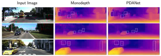
Figure 5.
Comparison between PDANet and Monodepth on KITTI 2015 [6]. PDANet achieves much better performance than Monodepth in terms of edges, land marks, and low-texture areas.
Table 3.
Evaluation indicators for depth estimation models, where presents the ground-truth depth, d denotes the predicted depth, and is the number of predicted depth.
4.3. Other Datasets
To demonstrate the generalization ability of our network, we use Cityscapes dataset [37] and Make3D dataset [38] for testing. Although these datasets are different in camera parameters, image resolution, etc., our network still achieves reliable results.
4.3.1. Cityscapes
The CityScapes dataset [37] uses stereo video sequences to record 50 different city street scenes, including 22,973 stereo pairs. We also applied our model to the Cityscapes for testing and obtain a better test result, as shown in Figure 6. We preprocessed the images by removing the hood part of the car and retain only the top 80% of the image. Although KITTI [6] and Cityscapes differ in image size, scene content, and camera parameters, our model still achieves superior results. The low-texture areas such as billboards are clearly predicted, and good predictions are obtained for objects such as cars and streetlights. All of these show that the PDANet has a strong generalization ability.
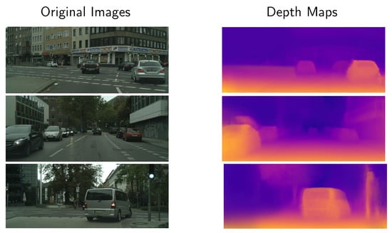
Figure 6.
Results on the Cityscapes dataset [37]. The strongly reflective Mercedes-Benz logo is removed and only the top 80% of the output image is retained.
4.3.2. Make3D
Make3D [38] consists of RGB monocular images and their depth maps, but stereo images are not available, so the unsupervised depth estimation model cannot be trained on this dataset. We therefore tested the Make3D with PDANet trained only on the KITTI, using the same camera parameters as those provided by the KITTI dataset. As a requirement of the aspect ratio of the images in the model, we cropped the input images. As shown in Table 4, the model achieves reasonable results, surpasses the baseline model, and even outperforms some supervised models in some metrics. The ground truth matrix of Make3D is too sparse, which prevents the supervised model from estimating the depth of each pixel properly. Our self-supervised learning method ignores this problem and obtains better depth results, as shown in Figure 7, although it cannot obtain numerically as good results as the supervised model.
Table 4.
Results on the Make3D dataset [38]. Losses are calculated on the cropped central images and the depth is lower than 70 m.
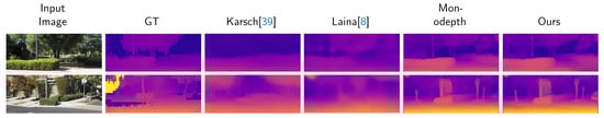
Figure 7.
Results and comparison on Make3D dataset [38].
4.4. Ablation Study
To present the impact of our data augmentation consistency and perceptual consistency improvement on the overall effect, an ablative analysis was implemented by combining different components. The quantitative results of different loss combinations are shown in Table 5. It shows that the prediction capability of the model improves with the addition of perceptual consistency and data augmentation consistency, and achieves the best results when the two components are integrated. Visualization of improvements by different components are shown in Figure 8, as shown in the blue patches, the edge performance, and detail representation significantly improve.
Table 5.
Ablation study of different components in PDANet.
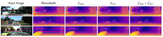
Figure 8.
Visualization of ablation study. From left to right: input images, the result of Monodepth, the result of Monodepth with data augmentation consistency, the result of Monodepth with perceptual consistency, and the result of PDANet, where is the data augmentation consistency loss and is the perceptual consistency loss. Blue patches show the different effects in detail when applying each module separately.
4.4.1. Effect of Perceptual Consistency
Perceptual loss uses multi-scale high-level features to optimize the contrast effect of reconstruction loss. It not only considers the differences between pixels but also reflects the differences in semantics. Large numbers of the input images with uneven illumination and shadows appear in the datasets, and the effect of prediction is significantly improved. As shown in Table 5, compared with the network without perceptual loss, the model with perceptual loss has a significant improvement in each indicator. Both of them contain the same data augmentation and reconstruction loss function, and the abs_rel error decreases from 0.0921 to 0.0846.
4.4.2. Effect of Data Augmentation Consistency
It is always necessary for unsupervised training to perform data augmentation, which improves the results of the self-supervised depth estimation network without affecting training time. As shown in Table 5, all indicators are better than the basic model. At the same time, data augmentation improves the generalization ability of the model and facilitates the migration of the model.
5. Conclusions
In this paper, we innovatively propose an unsupervised depth estimation method (PDANet) based on Monodepth. It aims at solving the problems of unreliable prediction caused by the color constancy hypothesis in the previous work of image reconstruction and the failure to obtain reliable image reconstruction loss in low-texture regions. The proposed method enforces the data augmentation consistency; consequently, the model has strong robustness in dealing with color interference. On the other hand, perceptual consistency solves the problem of image gradient disappearance in low-texture regions and enhances the consistency of reconstructed images at higher semantic levels. Experiments and ablation analysis on KITTI benchmark demonstrate the effectiveness of our unsupervised learning model. We also tested our model on Cityscapes and Make3D datasets and obtained superior results. Our model shows not only strong deep prediction capability but also generalization ability on different datasets.
Although our proposed perceptual consistency and data augmentation consistency improve the quality of the results, the method still has some limitations. Our model still fails to perform better when encountering transparent areas such as glass. Further, the training process of our model requires the input of two high-quality images with different perspectives to generate unsupervised signals, meaning that our model cannot be trained on a dataset with only a single perspective image.
In future work, we will extend our model to video by considering the relationship among multiple frames and ensuring the consistency of the same region among video frames. We will also further investigate the limitations mentioned above in subsequent research, improve the effectiveness of self-supervised depth estimation, bridge the gap between our method, and fully supervised learning methods.
Author Contributions
Conceptualization, H.G. and X.L.; methodology, H.G. and X.L.; validation, H.G., X.L., and M.Q.; writing—original draft preparation, H.G., M.Q., and S.H.; writing—review and editing, H.G., M.Q., and S.H.; visualization, H.G. and X.L.; supervision, M.Q.; funding acquisition, M.Q. All authors have read and agreed to the published version of the manuscript.
Funding
This paper was supported by the Shandong Provincial Natural Science Foundation, China (No. ZR2018MA032, ZR2020MA064).
Institutional Review Board Statement
Not applicable.
Informed Consent Statement
Not applicable.
Data Availability Statement
Data are not availability for public.
Conflicts of Interest
The authors declare no conflict of interest.
Abbreviations
The following abbreviations are used in this manuscript:
| SfM | Structure from Motion |
| SLAM | Simultaneous Localization and Mapping |
| VGG16 | Visual Geometry Group Network with 16 convolutional layers |
| LiDAR | Light Detection and Ranging |
| RGB | Red Green and Blue |
| CNN | Convolution Neural Network |
| Monodepth | Monocular Depth Estimation Network proposed by Godard et al. |
| SSIM | Structural Similarity |
| L1 | Least Absolute Deviation |
| PP | Post Processing |
| RMSE | Root Mean Square Error |
| abs_rel | Absolute Relative Error |
| sq_rel | Square Relative Error |
| GT | Ground Truth |
References
- Newcombe, R.A.; Lovegrove, S.J.; Davison, A.J. DTAM: Dense tracking and mapping in real-time. In Proceedings of the 2011 International Conference on Computer Vision, Barcelona, Spain, 6–13 November 2011; pp. 2320–2327. [Google Scholar]
- Kak, A.; DeSouza, G. Vision for mobile robot navigation. IEEE Trans. Pattern Anal. Mach. Intell. 2002, 24, 237–267. [Google Scholar]
- Menze, M.; Geiger, A. Object scene flow for autonomous vehicles. In Proceedings of the IEEE Conference on Computer Vision and Pattern Recognition, Boston, MA, USA, 7–12 June 2015; pp. 3061–3070. [Google Scholar]
- Engel, J.; Koltun, V.; Cremers, D. Direct sparse odometry. IEEE Trans. Pattern Anal. Mach. Intell. 2017, 40, 611–625. [Google Scholar] [CrossRef] [PubMed]
- Eigen, D.; Puhrsch, C.; Fergus, R. Depth map prediction from a single image using a multi-scale deep network. arXiv 2014, arXiv:1406.2283. [Google Scholar]
- Geiger, A.; Lenz, P.; Urtasun, R. Are we ready for autonomous driving? the kitti vision benchmark suite. In Proceedings of the 2012 IEEE Conference on Computer Vision and Pattern Recognition, Providence, RI, USA, 16–21 June 2012. [Google Scholar]
- Eigen, D.; Fergus, R. Predicting depth, surface normals and semantic labels with a common multi-scale convolutional architecture. In Proceedings of the IEEE International Conference on Computer Vision, Santiago, Chile, 7–13 December 2015; pp. 2650–2658. [Google Scholar]
- Laina, I.; Rupprecht, C.; Belagiannis, V.; Tombari, F.; Navab, N. Deeper depth prediction with fully convolutional residual networks. In Proceedings of the 2016 Fourth International Conference on 3D Vision (3DV), Stanford, CA, USA, 25–28 October 2016; pp. 239–248. [Google Scholar]
- Cao, Y.; Wu, Z.; Shen, C. Estimating depth from monocular images as classification using deep fully convolutional residual networks. IEEE Trans. Circuits Syst. Video Technol. 2017, 28, 3174–3182. [Google Scholar] [CrossRef]
- Fu, H.; Gong, M.; Wang, C.; Batmanghelich, K.; Tao, D. Deep ordinal regression network for monocular depth estimation. In Proceedings of the IEEE Conference on Computer Vision and Pattern Recognition, Salt Lake City, UT, USA, 18–22 June 2018; pp. 2002–2011. [Google Scholar]
- Zhan, H.; Garg, R.; Weerasekera, C.S.; Li, K.; Agarwal, H.; Reid, I. Unsupervised learning of monocular depth estimation and visual odometry with deep feature reconstruction. In Proceedings of the IEEE Conference on Computer Vision and Pattern Recognition, Salt Lake City, UT, USA, 18–22 June 2018; pp. 340–349. [Google Scholar]
- Chen, W.; Fu, Z.; Yang, D.; Deng, J. Single-image depth perception in the wild. arXiv 2016, arXiv:1604.03901. [Google Scholar]
- Wu, Y.; Ying, S.; Zheng, L. Size-to-depth: A new perspective for single image depth estimation. arXiv 2018, arXiv:1801.04461. [Google Scholar]
- Garg, R.; Bg, V.K.; Carneiro, G.; Reid, I. Unsupervised cnn for single view depth estimation: Geometry to the rescue. In Proceedings of the European Conference on Computer Vision, Amsterdam, The Netherlands, 11–14 October 2016; Springer: Berlin/Heidelberg, Germany, 2016; pp. 740–756. [Google Scholar]
- Godard, C.; Mac Aodha, O.; Brostow, G.J. Unsupervised monocular depth estimation with left-right consistency. In Proceedings of the IEEE Conference on Computer Vision and Pattern Recognition, Honolulu, HI, USA, 21–26 July 2017; pp. 270–279. [Google Scholar]
- Tosi, F.; Aleotti, F.; Poggi, M.; Mattoccia, S. Learning monocular depth estimation infusing traditional stereo knowledge. In Proceedings of the IEEE/CVF Conference on Computer Vision and Pattern Recognition, Long Beach, CA, USA, 15–20 June 2019; pp. 9799–9809. [Google Scholar]
- Wong, A.; Soatto, S. Bilateral cyclic constraint and adaptive regularization for unsupervised monocular depth prediction. In Proceedings of the IEEE/CVF Conference on Computer Vision and Pattern Recognition, Long Beach, CA, USA, 15–20 June 2019; pp. 5644–5653. [Google Scholar]
- Poggi, M.; Tosi, F.; Mattoccia, S. Learning monocular depth estimation with unsupervised trinocular assumptions. In Proceedings of the 2018 International Conference on 3D Vision (3DV), Verona, Italy, 5–8 September 2018; pp. 324–333. [Google Scholar]
- Pilzer, A.; Xu, D.; Puscas, M.; Ricci, E.; Sebe, N. Unsupervised adversarial depth estimation using cycled generative networks. In Proceedings of the 2018 International Conference on 3D Vision (3DV), Verona, Italy, 5–8 September 2018; pp. 587–595. [Google Scholar]
- CS Kumar, A.; Bhandarkar, S.M.; Prasad, M. Monocular depth prediction using generative adversarial networks. In Proceedings of the IEEE Conference on Computer Vision and Pattern Recognition Workshops, Salt Lake City, UT, USA, 18–22 June 2018; pp. 300–308. [Google Scholar]
- Zhai, M.; Xiang, X.; Lv, N.; Kong, X.; El Saddik, A. An object context integrated network for joint learning of depth and optical flow. IEEE Trans. Image Process. 2020, 29, 7807–7818. [Google Scholar] [CrossRef]
- Shu, C.; Yu, K.; Duan, Z.; Yang, K. Feature-metric loss for self-supervised learning of depth and egomotion. In Proceedings of the European Conference on Computer Vision, Glasgow, UK, 23–28 August 2020; Springer: Berlin/Heidelberg, Germany, 2020; pp. 572–588. [Google Scholar]
- Johnson, J.; Alahi, A.; Fei-Fei, L. Perceptual losses for real-time style transfer and super-resolution. In Proceedings of the European Conference on Computer Vision, Amsterdam, The Netherlands, 11–14 October 2016; Springer: Berlin/Heidelberg, Germany, 2016; pp. 694–711. [Google Scholar]
- Yang, G.; Zhao, H.; Shi, J.; Deng, Z.; Jia, J. Segstereo: Exploiting semantic information for disparity estimation. In Proceedings of the European Conference on Computer Vision (ECCV), Glasgow, UK, 8–14 September 2018; pp. 636–651. [Google Scholar]
- Liu, S.; Huang, D.; Wang, Y. Learning spatial fusion for single-shot object detection. arXiv 2019, arXiv:1911.09516. [Google Scholar]
- Xie, Q.; Dai, Z.; Hovy, E.; Luong, M.T.; Le, Q.V. Unsupervised data augmentation for consistency training. arXiv 2019, arXiv:1904.12848. [Google Scholar]
- Chen, T.; Kornblith, S.; Norouzi, M.; Hinton, G. A simple framework for contrastive learning of visual representations. In Proceedings of the International Conference on Machine Learning, PMLR, Cambridge, MA, USA, 13–18 July 2020; pp. 1597–1607. [Google Scholar]
- Dovesi, P.L.; Poggi, M.; Andraghetti, L.; Martí, M.; Kjellström, H.; Pieropan, A.; Mattoccia, S. Real-time semantic stereo matching. In Proceedings of the 2020 IEEE International Conference on Robotics and Automation (ICRA), Paris, France, 31 May–31 August 2020; pp. 10780–10787. [Google Scholar]
- Xu, D.; Wang, W.; Tang, H.; Liu, H.; Sebe, N.; Ricci, E. Structured attention guided convolutional neural fields for monocular depth estimation. In Proceedings of the IEEE Conference on Computer Vision and Pattern Recognition, Salt Lake City, UT, USA, 18–22 June 2018; pp. 3917–3925. [Google Scholar]
- Zhang, H.; Shen, C.; Li, Y.; Cao, Y.; Liu, Y.; Yan, Y. Exploiting temporal consistency for real-time video depth estimation. In Proceedings of the IEEE/CVF International Conference on Computer Vision, Seoul, Korea, 27 October–2 November 2019; pp. 1725–1734. [Google Scholar]
- Amiri, A.J.; Loo, S.Y.; Zhang, H. Semi-supervised monocular depth estimation with left-right consistency using deep neural network. In Proceedings of the 2019 IEEE International Conference on Robotics and Biomimetics (ROBIO), Dali, China, 6–8 December 2019; pp. 602–607. [Google Scholar]
- Ranjan, A.; Jampani, V.; Balles, L.; Kim, K.; Sun, D.; Wulff, J.; Black, M.J. Competitive collaboration: Joint unsupervised learning of depth, camera motion, optical flow and motion segmentation. In Proceedings of the IEEE/CVF Conference on Computer Vision and Pattern Recognition, Long Beach, CA, USA, 15–20 June 2019; pp. 12240–12249. [Google Scholar]
- Chen, P.Y.; Liu, A.H.; Liu, Y.C.; Wang, Y.C.F. Towards scene understanding: Unsupervised monocular depth estimation with semantic-aware representation. In Proceedings of the IEEE/CVF Conference on Computer Vision and Pattern Recognition, Long Beach, CA, USA, 15–20 June 2019; pp. 2624–2632. [Google Scholar]
- Zhou, J.; Wang, Y.; Qin, K.; Zeng, W. Unsupervised high-resolution depth learning from videos with dual networks. In Proceedings of the IEEE/CVF International Conference on Computer Vision, Seoul, Korea, 27 October–2 November 2019; pp. 6872–6881. [Google Scholar]
- Casser, V.; Pirk, S.; Mahjourian, R.; Angelova, A. Unsupervised monocular depth and ego-motion learning with structure and semantics. In Proceedings of the IEEE/CVF Conference on Computer Vision and Pattern Recognition Workshops, Long Beach, CA, USA, 15–20 June 2019. [Google Scholar]
- Chen, Y.; Schmid, C.; Sminchisescu, C. Self-supervised learning with geometric constraints in monocular video: Connecting flow, depth, and camera. In Proceedings of the IEEE/CVF International Conference on Computer Vision, Seoul, Korea, 27 October–2 November 2019; pp. 7063–7072. [Google Scholar]
- Cordts, M.; Omran, M.; Ramos, S.; Rehfeld, T.; Enzweiler, M.; Benenson, R.; Franke, U.; Roth, S.; Schiele, B. The cityscapes dataset for semantic urban scene understanding. In Proceedings of the IEEE conference on computer vision and pattern recognition, Las Vegas, NV, USA, 27–30 June 2016; pp. 3213–3223. [Google Scholar]
- Saxena, A.; Sun, M.; Ng, A.Y. Make3d: Learning 3d scene structure from a single still image. IEEE Trans. Pattern Anal. Mach. Intell. 2008, 31, 824–840. [Google Scholar] [CrossRef] [PubMed]
- Karsch, K.; Liu, C.; Kang, S.B. Depth transfer: Depth extraction from video using non-parametric sampling. IEEE Trans. Pattern Anal. Mach. Intell. 2014, 36, 2144–2158. [Google Scholar] [CrossRef] [PubMed]


Publisher’s Note: MDPI stays neutral with regard to jurisdictional claims in published maps and institutional affiliations. |
© 2021 by the authors. Licensee MDPI, Basel, Switzerland. This article is an open access article distributed under the terms and conditions of the Creative Commons Attribution (CC BY) license (https://creativecommons.org/licenses/by/4.0/).