
Artificial Neural Networks to Optimize Zero Energy Building (ZEB) Projects from the Early Design Stages


 and
and
Abstract
Featured Application
Abstract
1. Introduction and Research Scope
2. Literature Review
2.1. Energy Simulation Methods: Top-Down Approaches
2.2. Energy Simulation Methods: Bottom-Up Approaches
3. Research Scope in Relation to the Literature
3.1. The Gap
3.2. The Objective of the Research
- Running a very large amount of energy simulations of archetype buildings by varying a chosen set of their characteristics;
- Collecting all the energy simulation results into a single database;
- Using machine learning techniques to synthesize the database developed into the forecasting tools by means of ANNs.
4. Methodological Approach
4.1. ANN Target Characteristics
- Instantaneously recalculate the main seasonal energy needs when the user modifies the input parameters, such as overall sizes, window ratios and building constructions, via sliders in a graphical user interface (GUI);
- Adapt to various building occupation levels.
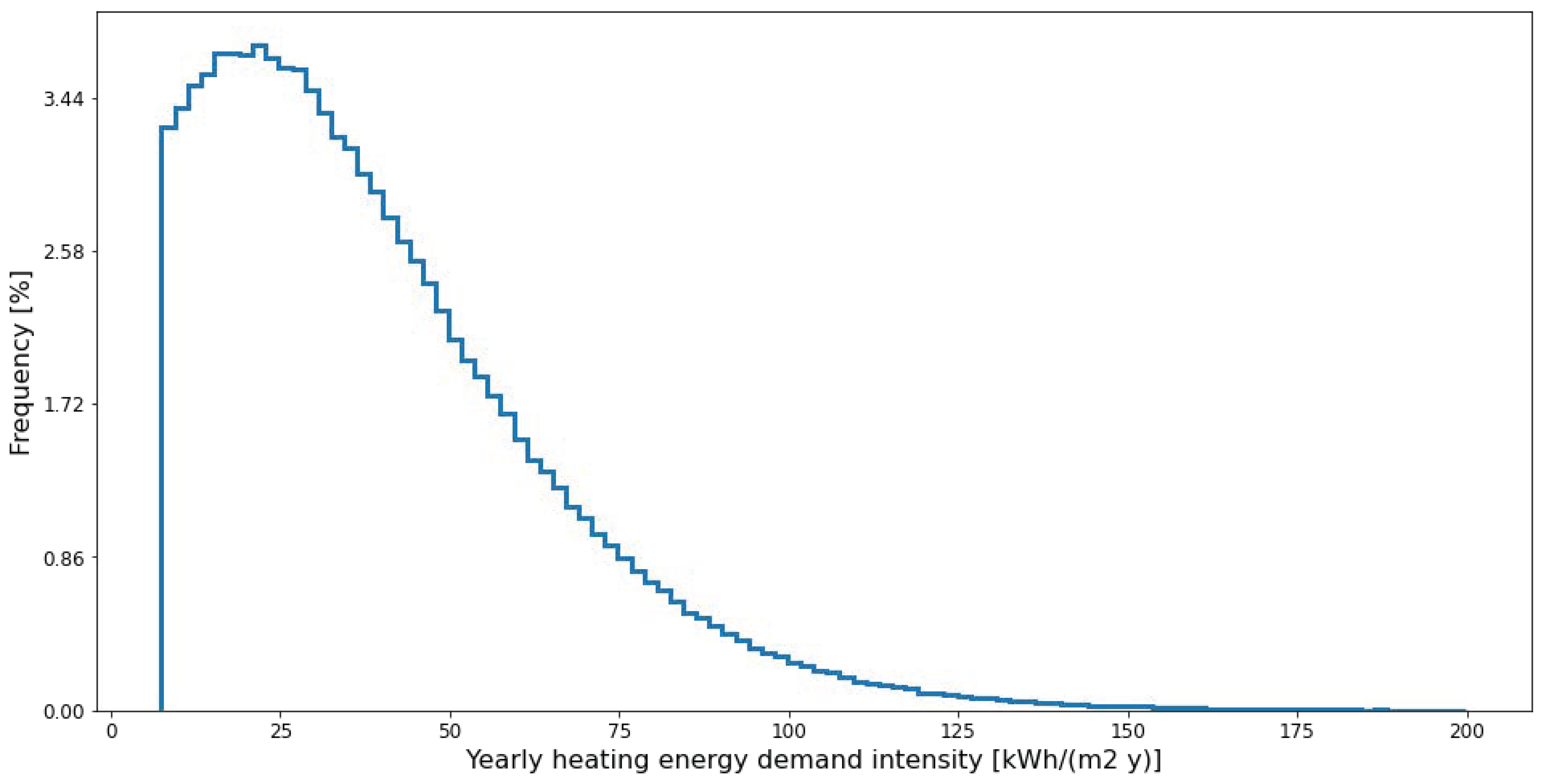
4.2. The Database to Train the Networks
- -
- Heating energy needs: 7/250 kWh/m2;
- -
- Cooling energy needs: 3/90 kWh/m2;
- -
- Domestic hot water preparation energy needs: 3/40 kWh/m2;
- -
- Lighting energy needs: 1/15 kWh/m2;
- -
- Other electrical appliances energy needs: 7/50 kWh/m2.
- Heating energy demand (kWh/y);
- Cooling energy demand (kWh/y);
- Lighting energy demand (kWh/y);
- Electrical equipment energy demand (kWh/y);
- Domestic hot water (DHW) energy demand (kWh/y);
- Total solar energy transmitted by the windows’ facing, with no regard to the building’s azimuth angle (kWh/(m2·y)):
- -
- North;
- -
- East;
- -
- South;
- -
- West;
- Yearly average value of illuminance in the center of the zone during occupancy hours (lux);
- Yearly average value of CO2 concentration in the zone during occupancy hours (ppm);
- Average zone air temperature in the period of December–January (i.e., in midwinter) during occupancy hours (°C);
- Average zone air relative humidity in the period of December–January during occupancy hours (%);
- Average zone air temperature in the period of June–July (i.e., in midsummer) during occupancy hours (°C);
- Average zone air relative humidity in the period of June–July during occupancy hours (%);
- Calculated design heating capacity (kW);
- Calculated design cooling capacity (kW).
4.3. Producing the Training Database
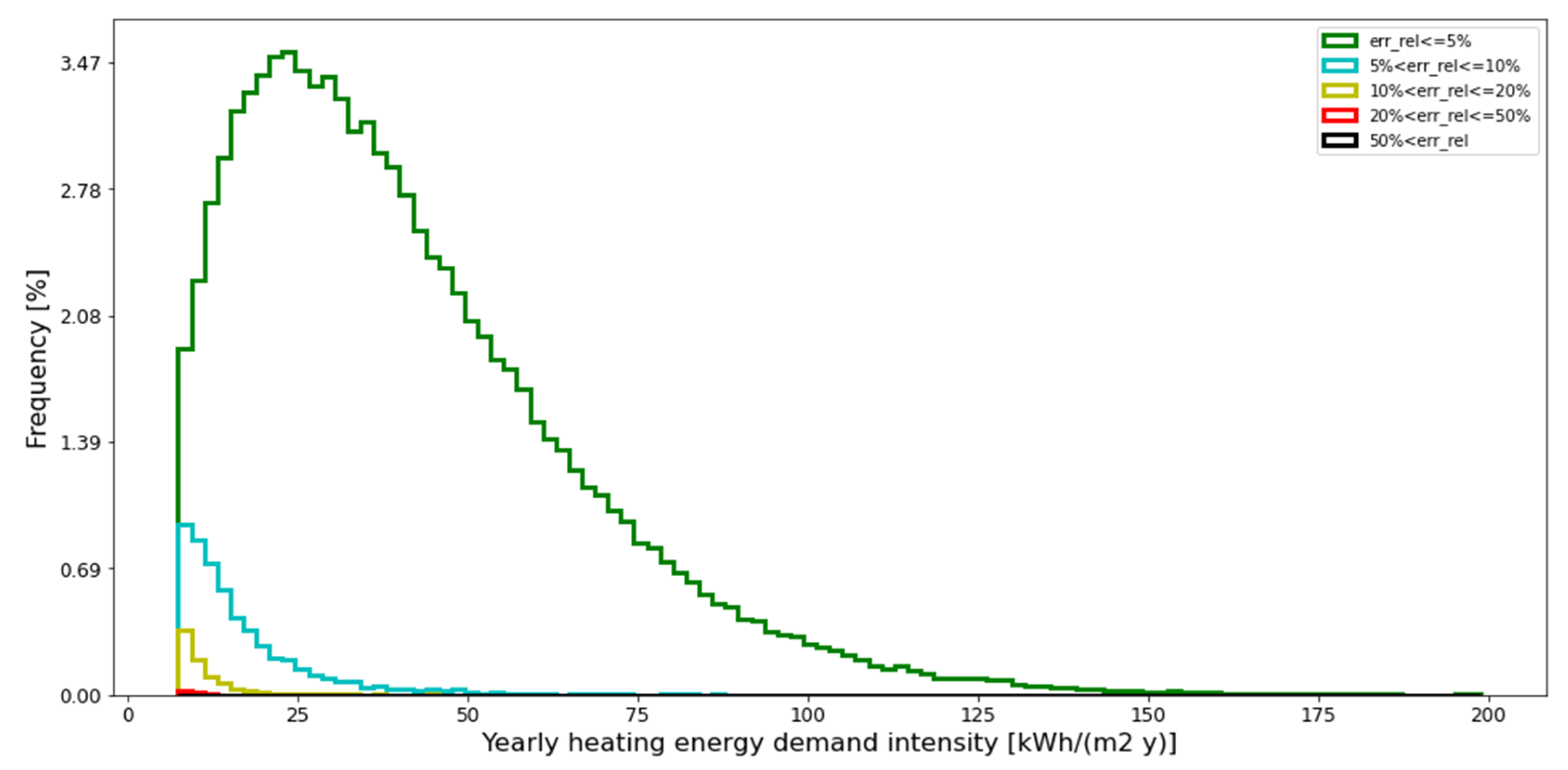
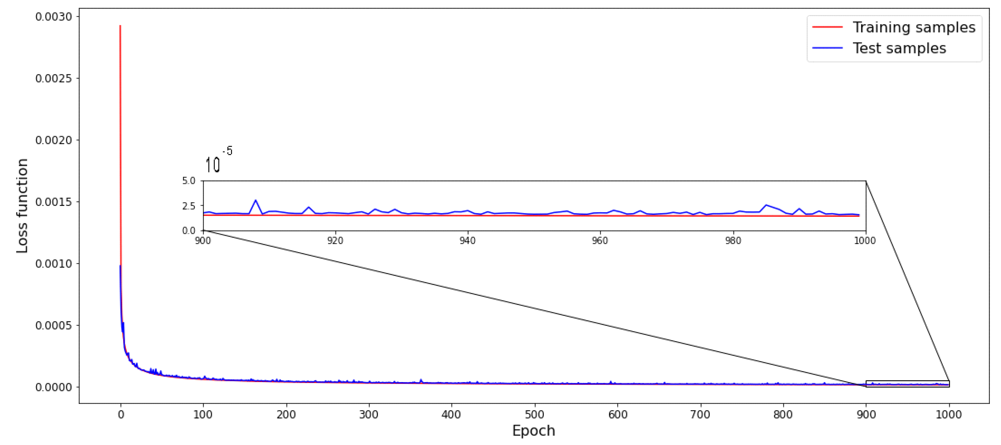
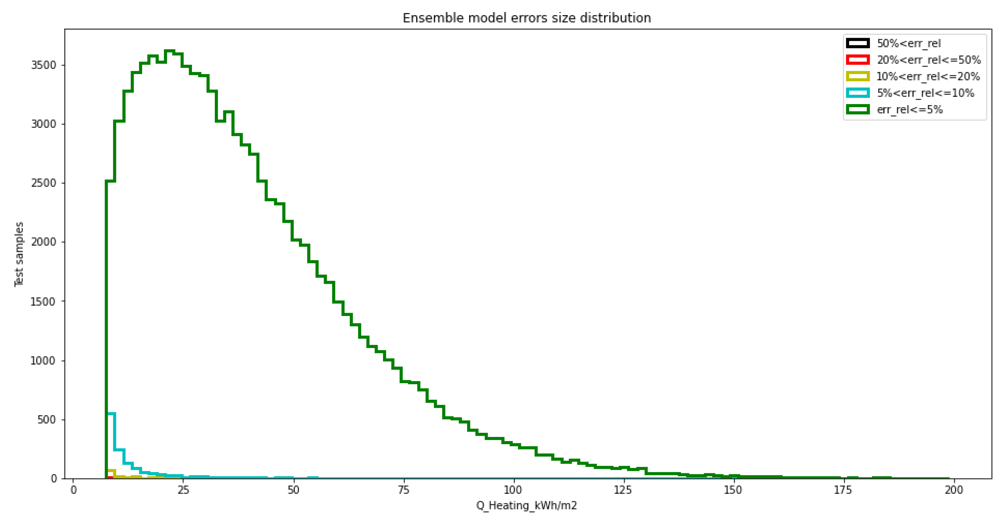
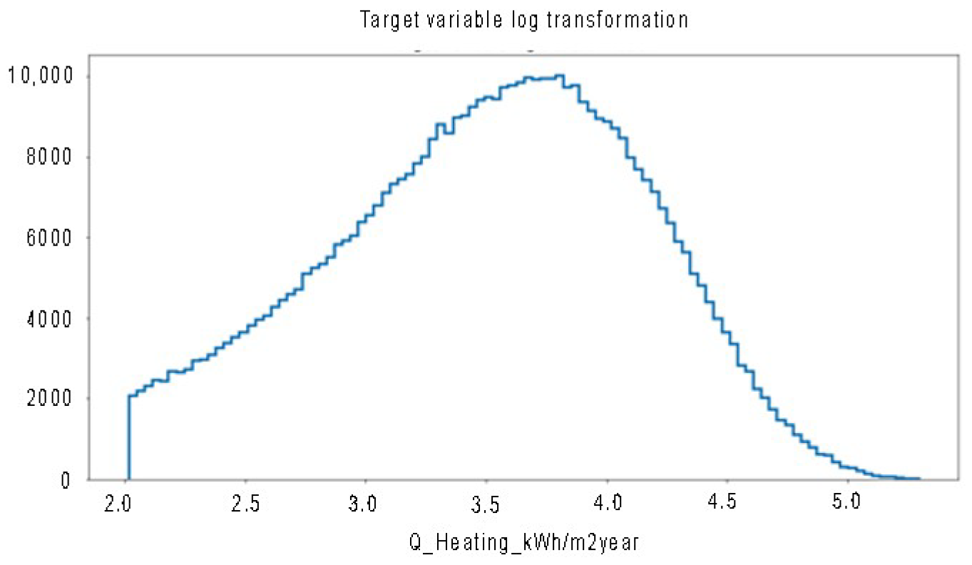
4.4. ANN Training and Accuracy Improvement
5. Results
5.1. The Developed Software
5.2. An Example of the Simulation Results
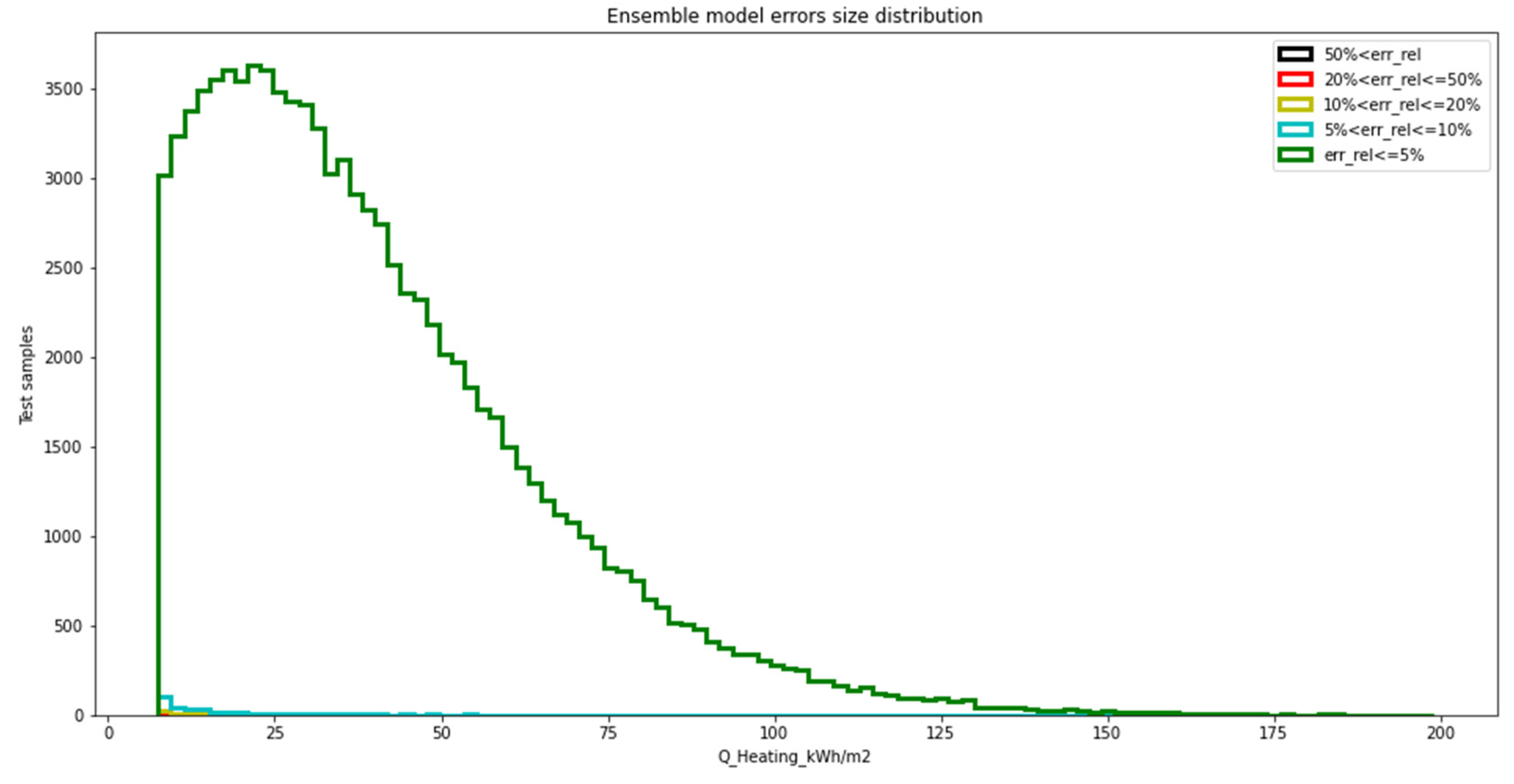
5.3. Identify the Best DFANN Complexity
- Number of hidden layers (Min/Max): 2/6;
- Number of nodes per layer (Min/Max): 60/280;
- Maximum number of epochs: 1000, saving the best model developed along the epochs;
- Number of DFANNs concurring with the ensemble model: 10.
6. Discussion and Further Improvements
6.1. Calculation Time
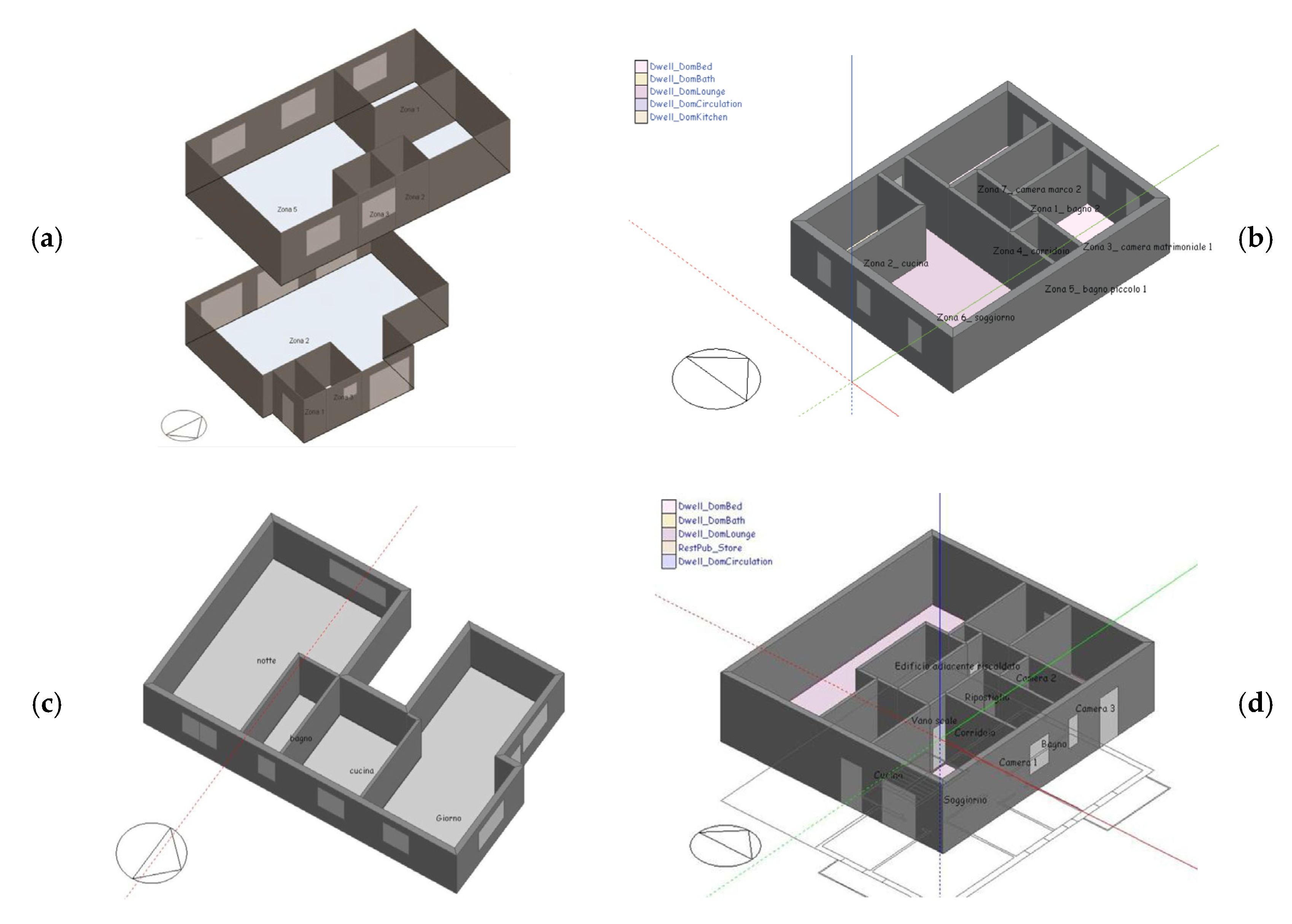
6.2. A Test on Illustrative Case Studies
7. Conclusions
Author Contributions
Funding
Institutional Review Board Statement
Informed Consent Statement
Conflicts of Interest
Nomenclature
| ANN | Artificial neural network |
| API | Application programming interface |
| BEM | Building energy modeling |
| BP | Backpropagation |
| DFANN | Deep feedforward artificial neural network |
| GUI | Graphical user interface |
| HVAC | Heating, ventilation and air-conditioning |
| IAQ | Indoor air quality |
| Idf | (EnergyPlus) input data file |
| PV | Photovoltaics |
| RNN | Recurrent neural network |
| ZEB | Zero-energy building |
References
- Marszal, A.J.; Heiselberg, P.; Bourrelle, J.S.; Musall, E.; Voss, K.; Sartori, I.; Napolitano, A. Zero Energy Building-A review of definitions and calculation methodologies. Energy Build. 2011, 43, 971–979. [Google Scholar] [CrossRef]
- Harvey, L.D.D. Recent Advances in Sustainable Buildings: Review of the Energy and Cost Performance of the State-of-the-Art Best Practices from Around the World. Annu. Rev. Environ. Resour. 2013, 38, 281–309. [Google Scholar] [CrossRef]
- Evins, R. A review of computational optimisation methods applied to sustainable building design. Renew. Sustain. Energy Rev. 2013, 22, 230–245. [Google Scholar] [CrossRef]
- Machairas, V.; Tsangrassoulis, A.; Axarli, K. Algorithms for optimization of building design: A review. Renew. Sustain. Energy Rev. 2014, 31, 101–112. [Google Scholar] [CrossRef]
- Li, W.; Zhou, Y.; Cetin, K.; Eom, J.; Wang, Y.; Chen, G.; Zhang, X. Modeling urban building energy use: A review of modeling approaches and procedures. Energy 2017, 141, 2445–2457. [Google Scholar] [CrossRef]
- Swan, L.G.; Ugursal, V.I. Modeling of end-use energy consumption in the residential sector: A review of modeling techniques. Renew. Sustain. Energy Rev. 2009, 13, 1819–1835. [Google Scholar] [CrossRef]
- Hirst, E.; Lin, W.; Cope, J. A residential energy use model sensitive to demographic, economic, and technological factors. Q. Rev. Econ. Financ. 1977, 17, 7–22. [Google Scholar]
- Haas, R.; Schipper, L. Residential energy demand in OECD-countries and the role of irreversible efficiency improvements. Energy Econ. 1998, 20, 421–442. [Google Scholar] [CrossRef]
- Zhang, Q. Residential energy consumption in China and its comparison with Japan, Canada, and USA. Energy Build. 2004, 36, 1217–1225. [Google Scholar] [CrossRef]
- Labanderia, X.; Labeaga, J.M.; Rodriguez, M. Policy Research A Residential Energy Demand System for Spain. Energy J. 2006, 27, 87–111. [Google Scholar]
- Summerfield, A.J.; Lowe, R.J.; Oreszczyn, T. Two models for benchmarking UK domestic delivered energy. Build. Res. Inf. 2010, 38, 12–24. [Google Scholar] [CrossRef]
- Nesbakken, R. Price sensitivity of residential energy consumption in Norway. Energy Econ. 1999, 21, 493–515. [Google Scholar] [CrossRef]
- Bentzen, J.; Engsted, T. A revival of the autoregressive distributed lag model in estimating energy demand relationships. Energy 2001, 26, 45–55. [Google Scholar] [CrossRef]
- Ozturk, H.K.; Canyurt, O.E.; Hepbasli, A.; Utlu, Z. Residential-commercial energy input estimation based on genetic algorithm (GA) approaches: An application of Turkey. Energy Build. 2004, 36, 175–183. [Google Scholar] [CrossRef]
- Saha, G.P.; Stephenson, J. A model of residential energy use in New Zealand. Energy 1980, 5, 167–175. [Google Scholar] [CrossRef]
- Fumo, N.; Rafe Biswas, M.A. Regression analysis for prediction of residential energy consumption. Renew. Sustain. Energy Rev. 2015, 47, 332–343. [Google Scholar] [CrossRef]
- Chidiac, S.E.; Catania, E.J.C.; Morofsky, E.; Foo, S. A screening methodology for implementing cost effective energy retrofit measures in Canadian office buildings. Energy Build. 2011, 43, 614–620. [Google Scholar] [CrossRef]
- Catalina, T.; Iordache, V.; Caracaleanu, B. Multiple regression model for fast prediction of the heating energy demand. Energy Build. 2013, 57, 302–312. [Google Scholar] [CrossRef]
- Amiri, S.S.; Mottahedi, M.; Asadi, S. Using multiple regression analysis to develop energy consumption indicators for commercial buildings in the U.S. Energy Build. 2015, 109, 209–216. [Google Scholar] [CrossRef]
- Parti, M.; Parti, C. The Total and Appliance-Specific Conditional Demand for Electricity in the Household Sector. Bell J. Econ. 1980, 11, 309–321. [Google Scholar] [CrossRef]
- Lafrance, G.; Perron, D. Evolution of Residential Electricity Demand by End-Use in Quebec 1979–1989: A Conditional Demand Analysis. Energy Stud. Rev. 1994, 6, 164–173. [Google Scholar] [CrossRef]
- Aydinalp-Koksal, M.; Ugursal, V.I. Comparison of neural network, conditional demand analysis, and engineering approaches for modeling end-use energy consumption in the residential sector. Appl. Energy 2008, 85, 271–296. [Google Scholar] [CrossRef]
- Matsumoto, S. How do household characteristics affect appliance usage? Application of conditional demand analysis to Japanese household data. Energy Policy 2016, 94, 214–223. [Google Scholar] [CrossRef]
- Park, D.C.; Marks, R.J.; Atlas, L.E.; Damborg, M.J. Electric load forecasting using an artificial neural network. IEEE Trans. Power Syst. 1991, 6, 442–449. [Google Scholar] [CrossRef]
- Aydinalp, M.; Ugursal, V.I.; Fung, A.S. Modeling of the appliance, lighting and space-cooling energy consumption in the residential sector using neural networks. Appl. Energy 2002, 71, 87–110. [Google Scholar] [CrossRef]
- Biswas, M.A.R.; Robinson, M.D.; Fumo, N. Prediction of residential building energy consumption: A neural network approach. Energy 2016, 117, 84–92. [Google Scholar] [CrossRef]
- Crawley, D.B.; Hand, J.W.; Kummert, M.; Griffith, B.T. Contrasting The Capabilities Of Building Energy Performance Simulation Programs. Build. Environ. 2008, 43, 661–673. [Google Scholar] [CrossRef]
- Fabbri, R.; Gabrielli, L.; Ruggeri, A.G. Interactions between restoration and financial analysis: The case of Cuneo War Wounded House. J. Cult. Herit. Manag. Sustain. Dev. 2018, 8, 145–161. [Google Scholar] [CrossRef]
- U.S. Department of Energy. EnergyPlus. 2015. Available online: www.energyplus.net (accessed on 25 May 2021).
- Klein, S.A.; Beckman, W.A.; Mitchell, J.W.; Duffie, J.A.; Duffie, N.A.; Freeman, T.L.; Mitchell, J.C.; Braun, J.E.; Evans, B.L.; Kummer, J.P.; et al. TRNSYS 16–TraNsient System Simulation Program, User Manual; Solar Energy Laboratory, University of Wisconsin-Madison: Madison, WI, USA, 2004. [Google Scholar]
- Tabatabaei Sameni, S.M.; Gaterell, M.; Montazami, A.; Ahmed, A. Overheating investigation in UK social housing flats built to the Passivhaus standard. Build. Environ. 2015, 92, 222–235. [Google Scholar] [CrossRef]
- Morgan, C.; Foster, J.A.; Poston, A.; Sharpe, T.R. Overheating in Scotland: Contributing factors in occupied homes. Build. Res. Inf. 2016. [Google Scholar] [CrossRef]
- Nowoświat, A.; Pokorska-Silva, I. The influence of thermal mass on the cooling off process of buildings. Period. Polytech. Civ. Eng. 2018, 62, 173–179. [Google Scholar] [CrossRef]
- Zinzi, M.; Pagliaro, F.; Agnoli, S.; Bisegna, F.; Iatauro, D. Assessing the overheating risks in Italian existing school buildings renovated with nZEB targets. Energy Procedia 2017, 142, 2517–2524. [Google Scholar] [CrossRef]
- Athienitis, A.; O’Brien, W. (Eds.) Modeling, Design, and Optimization of Net-Zero Energy Buildings; Ernst&Sohn: Berlin, Germany, 2015; ISBN 9783433030400. [Google Scholar]
- Østergård, T.; Jensen, R.L.; Maagaard, S.E. Building simulations supporting decision making in early design-A review. Renew. Sustain. Energy Rev. 2016, 61, 187–201. [Google Scholar] [CrossRef]
- Nord, N.; Tereshchenko, T.; Qvistgaard, L.H.; Tryggestad, I.S. Influence of occupant behavior and operation on performance of a residential Zero Emission Building in Norway. Energy Build. 2018, 159, 75–88. [Google Scholar] [CrossRef]
- Augenbroe, G. Trends in building simulation. Build. Environ. 2002, 37, 891–902. [Google Scholar] [CrossRef]
- Attia, S. State of the art of existing early design simulation tools for net zero energy buildings: A comparison of ten tools. Leed Ap 2011, 1–45. [Google Scholar] [CrossRef]
- Attia, S.; Eleftheriou, P.; Xeni, F.; Morlot, R.; Ménézo, C.; Kostopoulos, V.; Betsi, M.; Kalaitzoglou, I.; Pagliano, L.; Cellura, M.; et al. Overview and future challenges of nearly zero energy buildings (nZEB) design in Southern Europe. Energy Build. 2017, 155, 439–458. [Google Scholar] [CrossRef]
- Kalema, T.; Jhannesson, G.; Pylsy, P.; Hagengran, P. Accuracy of energy analysis of buildings: A comparison of a monthly energy balance method and simulation methods in calculating the energy consumption and the effect of thermal mass. J. Build. Phys. 2008, 32, 101–130. [Google Scholar] [CrossRef]
- ONNX. Available online: www.onnx.ai (accessed on 25 May 2021).
- Box, G.E.; Cox, D.R. An analysis of transformations revisited, rebutted. J. Am. Stat. Assoc. 1982, 77, 209–210. [Google Scholar] [CrossRef]
- Yeo, I.-K.; Johnson, R. A new family of power transformations to improve normality or symmetry. Biometrika 2000, 87, 954–959. [Google Scholar] [CrossRef]


| Code | Description | Unit | Range of Values | Notes | |
|---|---|---|---|---|---|
| Geometry and Layout | X | Length of side 1 of the floor | m | Minimum value: 7 Maximum value: 30 | |
| Y | Length of side 2 of the floor | m | Minimum value: 7 Maximum value: 30 | ||
| nStoreys | Number of stories | - | Minimum value: 1 Maximum value: 8 | ||
| α | Building’s azimuth | - | Minimum value: 0 Maximum value: 90 | ||
| FW,A,N | Window area fraction along north side (@ Building azimuth = 0°) | - | Minimum value: 0.01 Maximum value: 0.90 | ||
| FW,A,E | Window area fraction along east side (@ Building azimuth = 0°) | - | Minimum value: 0.01 Maximum value: 0.90 | ||
| FW,A,S | Window area fraction along south side (@ Building azimuth = 0°) | - | Minimum value: 0.01 Maximum value: 0.90 | ||
| FW,A,W | Window area fraction along west side (@ Building azimuth = 0°) | - | Minimum value: 0.01 Maximum value: 0.90 | ||
| Constructions | EWTh2 | External wall construction: thickness of the insulation layer | m | Minimum value: 0.00 Maximum value: 0.20 | For further details, please see Table 2. |
| EWTh3 | External wall construction: thickness of the masonry or concrete layer | m | Minimum value: 0.20 Maximum value: 0.40 | ||
| EWTC3 | External wall construction: thermal conductivity of the masonry or concrete layer | W/(m·K) | Minimum value: 0.60 Maximum value: 1.80 | ||
| RTh2 | Roof construction: thickness of the insulation layer | m | Minimum value: 0.00 Maximum value: 0.20 | ||
| FTh2 | Floor construction: thickness of the insulation layer | m | Minimum value: 0.00 Maximum value: 0.20 | ||
| G | Glazing type | String | G1, G2, G2Le, G3Le | For further details, please see Table 3. | |
| AII | Average infiltration flow rate intensity | ach | Minimum value: 0.01 Maximum value: 1.00 | ||
| Occupancy-Related Data | PD | People density | np/m2 | Minimum value: 0.02 Maximum value: 0.08 | For further details, please see Table 5. |
| LD | Density of electric consumption due to lights | W/m2 | Minimum value: 0 Maximum value: 6 | ||
| ED | Density of electric consumption due to electric equipment | W/m2 | Minimum value: 0 Maximum value: 20 | ||
| DHWI | Domestic hot water intensity | W/p | Minimum value: 0 Maximum value: 200 | ||
| AVI | Average ventilation flow rate intensity | m³/(s·p) | Minimum value: 0.001 Maximum value: 0.010 | - |
| Construction | Layer (-) | Thickness (m) | Thermal Conductivity (W/(m·K)) | Density (kg/m³) | Specific Heat (J/(kg·K)) | Thermal Resistance (m2·K/W) | Total Thermal Conductance (W/(m2·K)) |
|---|---|---|---|---|---|---|---|
| External wall | 01 (Ext) | 0.015 | 0.55 | 1500 | 900 | 0.027 | 0.15–6.04 |
| 02 | 0.000–0.200 | 0.034 | 45 | 900 | 0.000–5.882 | ||
| 03 | 0.200–0.400 | 0.600–1.800 | 1500 | 900 | 0.111–0.667 | ||
| 04 (Int) | 0.015 | 0.55 | 1500 | 900 | 0.027 | ||
| Roof | 01 (Ext) | 0.02 | 0.4 | 700 | 2500 | 0.050 | 0.15–1.28 |
| 02 | 0.000–0.200 | 0.034 | 45 | 900 | 0.000–5.882 | ||
| 03 | - | - | - | - | 0.16 | ||
| 04 | 0.3 | 0.55 | 1500 | 900 | 0.545 | ||
| 05 (Int) | 0.015 | 0.55 | 1500 | 900 | 0.027 | ||
| Floor | 01 (Ext) | 0.3 | 1.6 | 1800 | 900 | 0.188 | 0.16–3.83 |
| 02 | 0.000–0.200 | 0.034 | 100 | 900 | 0.000–5.882 | ||
| 03 | 0.1 | 1.6 | 1800 | 900 | 0.063 | ||
| 04 (Int) | 0.02 | 1.8 | 1800 | 900 | 0.011 |
| Code (Alpha) | Description (Alpha) | U-Value (W/(m2·K)) | Visible Transmittance (-) | Solar Heat Gain Coefficient (-) | |
|---|---|---|---|---|---|
| Glazing types | G1 | Single glazing | 5.70 | 0.86 | 0.90 |
| G2 | Double glazing | 2.70 | 0.76 | 0.81 | |
| G2Le | Double glazing, argon-filled, low emissivity film for solar gain | 1.10 | 0.63 | 0.72 | |
| G3Le | Triple glazing, argon-filled, low emissivity film for solar gain | 0.70 | 0.35 | 0.58 |
| Scope | Weekdays | All Other Days | ||
|---|---|---|---|---|
| Time Period | Control Temperature (°C) | Time Period | Control Temperature (°C) | |
| Heating | 00:00–08:00 | 16.0 | 00:00–08:00 | 16.0 |
| 08:00–24:00 | 20.0 | 08:00–24:00 | 20.0 | |
| Cooling | 00:00–08:00 | 30.0 | 00:00–08:00 | 30.0 |
| 08:00–24:00 | 28.0 | 08:00–24:00 | 28.0 | |
| Category | Weekdays | All Other Days | ||
|---|---|---|---|---|
| Time | Percentage | Time | Percentage | |
| People | 00:00–08:00 | 100% | 00:00–14:00 | 100% |
| 08:00–18:00 | 33% | 14:00–22:00 | 33% | |
| 18:00–24:00 | 100% | 22:00–24:00 | 100% | |
| Lights | 00:00–08:00 | 0% | 00:00–14:00 | 0% |
| 08:00–18:00 | 0% | 14:00–18:00 | 100% | |
| 18:00–24:00 | 100% | 18:00–24:00 | 100% | |
| Electric equipment | 00:00–08:00 | 20% | 00:00–14:00 | 20% |
| 08:00–18:00 | 30% | 14:00–22:00 | 100% | |
| 18:00–24:00 | 100% | 22:00–24:00 | 100% | |
| Domestic hot water | 00:00–08:00 | 0% | 00:00–14:00 | 0% |
| 08:00–18:00 | 20% | 14:00–22:00 | 20% | |
| 18:00–24:00 | 100% | 22:00–24:00 | 100% | |
| Model ID [-] | Hidden Layers [-] | Nodes Per Layer [-] | Train Loss [-] | Test Loss [-] | Best Epoch [-] | Training Time [s] |
|---|---|---|---|---|---|---|
| 1 | 2 | 140 | 2.81 × 10⁻⁵ | 2.85 × 10⁻⁵ | 992 | 25,285 |
| 2 | 2 | 280 | 2.25 × 10⁻⁵ | 2.35 × 10⁻⁵ | 997 | 29,470 |
| 3 | 3 | 140 | 2.01 × 10⁻⁵ | 2.03 × 10⁻⁵ | 992 | 28,062 |
| 4 | 3 | 280 | 1.66 × 10⁻⁵ | 1.82 × 10⁻⁵ | 995 | 34,723 |
| 5 | 4 | 140 | 1.83 × 10⁻⁵ | 1.89 × 10⁻⁵ | 997 | 30,525 |
| 6 | 4 | 280 | 1.40 × 10⁻⁵ | 1.54 × 10⁻⁵ | 999 | 39,641 |
| 7 | 5 | 140 | 1.67 × 10⁻⁵ | 1.73 × 10⁻⁵ | 995 | 33,096 |
| 8 | 5 | 280 | 1.31 × 10⁻⁵ | 1.51 × 10⁻⁵ | 984 | 43,685 |
| 9 | 6 | 140 | 1.55 × 10⁻⁵ | 1.63 × 10⁻⁵ | 993 | 34,988 |
| 10 | 6 | 280 | 1.23 × 10⁻⁵ | 1.50 × 10⁻⁵ | 996 | 50,064 |
| Relative Error (%) | Share of Training Samples (%) | Share of Test Samples (%) |
|---|---|---|
| 0–5 | 94.2747 | 93.7016 |
| 5–10 | 4.9558 | 5.4067 |
| 10–20 | 0.7379 | 0.8515 |
| 20–50 | 0.0315 | 0.0396 |
| 50+ | 0.0000 | 0.0007 |
| Relative Error (%) | Share of Training Samples (%) | Share of Test Samples (%) |
|---|---|---|
| 0–5 | 98.4793 | 92.9048 |
| 5–10 | 1.3417 | 5.9539 |
| 10–20 | 0.1585 | 1.0656 |
| 20–50 | 0.0205 | 0.0757 |
| 50+ | 0.0000 | 0.0000 |
| Relative Error (%) | Share of Test Samples (%) |
|---|---|
| 0–5 | 99.5009 |
| 5–10 | 0.3958 |
| 10–20 | 0.0982 |
| 20–50 | 0.0051 |
| 50+ | 0.0000 |
| Number of Predictions in the Batch (-) | 1 | 10 | 100 | 1000 |
|---|---|---|---|---|
| Time of Execution (s) | 0.023 | 0.026 | 0.033 | 0.123 |
| Code | Zone | Floor Area | North Façade | East Façade | South Façade | West Façade | Heating Energy Consumption (by ANN) | Heating Energy Consumption (Simulated) | Error | ||||
|---|---|---|---|---|---|---|---|---|---|---|---|---|---|
| Total | Windows | Total | Windows | Total | Windows | Total | Windows | ||||||
| m2 | m2 | m2 | m2 | m2 | m2 | m2 | m2 | m2 | kWh/m2-y | kWh/m2-y | % | ||
| Building a | Padua | 144 | 69 | 25 | 40 | 0 | 69 | 14 | 40 | 0 | 14.4 | 13.90 | 3.60% |
| Building b | Padua | 110 | 51 | 0 | 35 | 5 | 51 | 0 | 35 | 4 | 12.2 | 13.1 | −6.87% |
| Building c | Vicenza | 127 | 30 | 7 | 40 | 8 | 25 | 0 | 43 | 4 | 16.8 | 16.1 | 4.35% |
| Building d | Ravenna | 84 | 22 | 2 | 41 | 6 | 22 | 7 | 41 | 0 | 18.1 | 17.8 | 1.69% |
Publisher’s Note: MDPI stays neutral with regard to jurisdictional claims in published maps and institutional affiliations. |
© 2021 by the authors. Licensee MDPI, Basel, Switzerland. This article is an open access article distributed under the terms and conditions of the Creative Commons Attribution (CC BY) license (https://creativecommons.org/licenses/by/4.0/).
Share and Cite
Pittarello, M.; Scarpa, M.; Ruggeri, A.G.; Gabrielli, L.; Schibuola, L. Artificial Neural Networks to Optimize Zero Energy Building (ZEB) Projects from the Early Design Stages. Appl. Sci. 2021, 11, 5377. https://doi.org/10.3390/app11125377
Pittarello M, Scarpa M, Ruggeri AG, Gabrielli L, Schibuola L. Artificial Neural Networks to Optimize Zero Energy Building (ZEB) Projects from the Early Design Stages. Applied Sciences. 2021; 11(12):5377. https://doi.org/10.3390/app11125377
Chicago/Turabian StylePittarello, Marco, Massimiliano Scarpa, Aurora Greta Ruggeri, Laura Gabrielli, and Luigi Schibuola. 2021. "Artificial Neural Networks to Optimize Zero Energy Building (ZEB) Projects from the Early Design Stages" Applied Sciences 11, no. 12: 5377. https://doi.org/10.3390/app11125377
APA StylePittarello, M., Scarpa, M., Ruggeri, A. G., Gabrielli, L., & Schibuola, L. (2021). Artificial Neural Networks to Optimize Zero Energy Building (ZEB) Projects from the Early Design Stages. Applied Sciences, 11(12), 5377. https://doi.org/10.3390/app11125377