Featured Application
The Artificial Neural Networks developed could be very useful for a fast and reliable assessment of buildings energy consumption without the use of specific energy simulation software.
Abstract
Building energy modeling (BEM) is used to support (nearly) zero-energy building (ZEB) projects, since this kind of software represents the only available option to forecast building energy consumption with high accuracy. BEM may also be used during preliminary analyses or feasibility studies, but simulation results are usually too detailed for this stage of the project. Aside from that, when optimization algorithms are used, the implied high number of energy simulations causes very long calculation times. Therefore, designers could be discouraged from the extensive use of BEM to conduct optimization analyses. Thus, they prefer to study and compare a very limited amount of acknowledged alternative designs. In relation to this problem, the scope of the present study is to obtain an easy-to-use tool to quickly forecast the energy consumption of a building with no direct use of BEM to support fast comparative analyses at the early stages of energy projects. In response, a set of automatic energy assessment tools was developed based on machine learning techniques. The forecasting tools are artificial neural networks (ANNs) that are able to estimate the energy consumption automatically for any building, based on a limited amount of descriptive data of the property. The ANNs are developed for the Po Valley area in Italy as a pilot case study. The ANNs may be very useful to assess the energy demand for even a considerable number of buildings by comparing different design options, and they may help optimization analyses.
1. Introduction and Research Scope
The design of zero-energy buildings (ZEBs) [1] is aimed at the achievement of the highest energy performance level in buildings, therefore leading to the lowest energy demand as well as the lowest operating costs due to energy consumption.
On the other hand, reaching ZEB standards also implies extra costs in construction, which may increase by up to 15% [2].
However, an excellent energy performance level similar to ZEB standards may also be reached through cost-effective design choices, finding the optimal balance between energy consumption and local generation. For instance, slightly higher energy consumption may be accepted in order to save the cost of construction due to the building envelope or heating, ventilation and air-conditioning (HVAC) system.
Aside from that, when pondering energy design choices, several limits and constraints must also be taken into account, such as the maximum area available to install the photovoltaics (PV) system, the maximum volume of the biofuel tanks or the maximum thickness of the walls. A wise building energy designer is able to manage this design complexity, but still, the project configuration he or she chooses may not be the best solution among all the feasible possibilities. In fact, achieving the optimal solution requires evaluating such a huge number of design parameters and alternative configurations that it seems unrealistic to be managed without the help of an automated multi-criteria optimization tool.
In order to achieve the best feasible building–system configuration, energy optimization tools should therefore be used from the early design phases [3,4]. Nonetheless, during the early design steps, such as in feasibility analyses, a plethora of design parameters still needs to be defined, typically pertaining to both building geometry and construction. Therefore, a lot of alternative design configurations should be compared so as to make the optimal choices. This is even more important if we consider that energy projects should also embed lighting, comfort and indoor air quality assessments in addition to the energy consumption forecasts. Moreover, these kinds of analyses should also be coupled with at least financial payback estimations or life cycle assessments in order to identify the most cost-effective configuration, since economic feasibility obviously plays a huge role in energy projects.
In this context, the authors of the present research paper suggest developing a set of automatic energy assessment tools based on machine learning techniques. These forecasting tools are meant to automatically estimate the energy consumption for any building on the basis of a limited amount of descriptive data of the property, which is suitable for the early design stages in a project. The aim is to provide an easy-to-use and extremely fast energy forecasting tool that can easily be used during the preliminary energy assessments of a project, as well as in comparative analyses or even in tandem with optimization procedures.
In particular, the authors have developed several artificial neural networks (ANNs) to forecast the main contributions to a building’s yearly energy consumption, such as heating needs, cooling needs, electricity consumption, contribution from ventilation air flow rates, solar gains and the building envelope. The ANNs developed could be very useful in the fast assessment of the energy demand for a building or even for a considerable number of buildings together, allowing the comparison of different design options and helping with identifying the optimal energy project among multiple alternatives.
This research is focussed on the Po Valley area in Northern Italy, which is a zone with homogeneous weather characteristics and hosts a population of about 20 million inhabitants today.
2. Literature Review
Energy assessment methodologies, as far as the current scientific literature is concerned, could be categorized into top-down and bottom-up strategies [5]. Top-down approaches assess the energy consumption in relation to its major macroeconomic drivers, while bottom-up methods evaluate the energy consumption related to more specific end-use information.
2.1. Energy Simulation Methods: Top-Down Approaches
Top-down approaches analyse a large group of buildings as if they were one single unit and study the interactions between energy use and the economy, population, technology or climate. A huge number of external factors are, in fact, significant in the determination of energy consumption and production. Such factors include, to name a few, demographic growth, macroeconomic indicators, market, construction and demolition rates, policy transformations, energy price, weather, consumer preferences and technological innovation [6]. In other words, top-down strategies capture the relationship between energy use and its major drivers, which is what makes these approaches extremely useful for estimating energy consumption at an urban scale, when it is crucial to determine the effects on the energy demand due to ongoing long-term changes. Top-down models are based on statistical inference, and they can be categorized according to the variables analyzed (e.g., economic, technology, physical or mixed variables). Econometric models are primarily based on prices and incomes. Economic variables may comprehend social or economic conditions, and they capture the effects of policies and market trends on energy use. Technological models link energy consumption to the widespread characteristics of the stock, while physical models rely on climate, weather and temperatures. One of the first applications of a top-down approach can be found in Hirst et al. [7], where the authors developed an econometric model to assess residential energy use over time. Their model was sensitive to changes in technology, population and the economy. Other top-down approaches for energy consumption estimation have been developed for several countries, such as the USA, Japan, Sweden, Germany, the UK [8,9,10,11], Norway [12], Denmark [13], China, Canada, Spain [12], Turkey [14] and New Zealand [15].
Top-down models only use aggregate data, which is both a strength and a weakness. On the one hand, aggregate data are easier to collect, and no detailed analysis of buildings is required. Moreover, they are able to include historical information, producing models very reliable for describing aggregated trends for future predictions in a stationary market, capturing the long-term effects of macroeconomic phenomena on energy demand. On the other hand, they do not provide appropriate predictions if significant changes happen in the economy, technological innovation or climate. Historical data give inertia to the model, and significant errors may occur because social, economic and weather conditions are likely to change over time. Most importantly, top-down methods cannot give sufficient knowledge about single buildings or single energy end uses, and they can only represent energy consumptions at an aggregate level.
To sum up, top-down methodologies are preferred when the objective is to underline the connection between energy use and different socioeconomic aspects. As much as those techniques are very useful for urban, regional and national planning and large-scale modeling, the building designer cannot rely on them for identifying specific areas to be enhanced or for scheduling energy efficiency interventions if our analysis works at a portfolio level.
2.2. Energy Simulation Methods: Bottom-Up Approaches
Bottom-up approaches relate energy consumption to more detailed buildings’ characteristics, such as systems and installations, geometry and shape, the thermodynamic properties of construction materials, external climate, indoor set-point temperatures, occupancy and relevant schedules. Since the level of a building’s knowledge is highly detailed, the accuracy of the estimate allows for a reliable assessment of the energy demand at the single-building scale.
Bottom-up approaches can still be divided into two different categories [5]: statistical methods and engineering methods. Statistical methods identify the relationship between buildings’ characteristics and their energy demand, relying on statistical inference. These approaches work similar to top-down strategies, sharing the strength of those techniques in applicability and straightforwardness, even though they use disaggregated data. Statistical methods include regression models, conditional demand analyses and artificial neural networks.
Regression analysis is a reliable and fast method to assess the energy demand in buildings. It is based on the determination of the statistical predictors, which are expected to influence the energy consumption of a building. A comprehensive discussion on the use of regression analyses to predict energy consumption in the residential sector can be found in the work of Fumo and Rafe Biswas [16], where the authors compared simple, multiple and multivariate linear regressions against non-linear regression models. Other works studied the complex selection process of predictors (i.e., independent variables), such as in the work of Chidiac et al. [17] for the Canadian office building stock, the work of Catalina et al. [18] for three different climatic zones (Moscow, Bucharest and Nice) and the work of Amiri et al. [19] for commercial buildings in the U.S.
Conditional demand analysis (CDA) is another statistical technique for modeling buildings’ energy demand which performs a regression that splits the energy consumption into contributions given by each end use appliance. In CDA approaches, the energy requirement is expressed as a sum of the energy consumption referring to each of the appliances working in the building. Thus, energy demand is directly related to equipment features, building characteristics or utilization patterns like thermostat settings or occupant behavior. Since the CDA runs a regression based on end uses, information is collected through surveys and utility data. A CDA was first employed in the work of Parti and Parti [20], where the authors presented a set of twelve cross-section regression analyses representing the monthly household demand for electricity in San Diego. Other interesting applications can be found in a study by Lafrance and Perron [21], where a CDA regression method was applied to electricity consumption in Québec, Aydinalp-Koksal and Ugursal [22], in which the authors modeled the energy use for Canada at a national-level, and in a study by Matsumoto [23], where the CDA was applied to Japanese household consumption.
The artificial neural network (ANN), or simply the neural network (NN), is a mathematical model inspired by the functioning of biological connections between the neurons in animals’ brains which grants learning processes. An NN builds a parallel mathematical model based on the interconnected structure of biological neural networks. The NN technique for modeling an individual building’s energy consumption originated and evolved in the 1990s. The work of Park et al. [24] contains one of the first applications of an ANN to forecast the electric load in the Seattle and Tacoma area. Later, Aydinalp et al. [25] developed an NN model to predict the Canadian residential energy consumption. They stated that NN techniques are highly suitable for determining causal relationships among a large number of parameters. More recently, Biswas et al. [26] created an NN to assess residential building energy consumption based on the case study of the TxAIRE Research and Demonstration House.
Finally, engineering physics-based methods simulate, with the help of simulation engines, the building’s energy consumption through the study of the thermodynamic properties that determine how the building, as a thermodynamic system, interacts with the outdoor environment [27]. Engineering methods are the most accurate ones, but they also require an intimate knowledge of the buildings. It is necessary to collect a plethora of information about their geometry, shape, orientation, glazing, materials, infiltration and ventilation rates, occupancy, schedules, internal loads, installations, set-point temperature and several other building characteristics and features. A concrete knowledge of the climatic area in which the building is located is also required, comprising microclimatic conditions and local effects [28]. More precisely, engineering physics-based methods can be categorized into steady state building energy assessment tools, dynamic building energy simulation tools and other building energy assessment tools.
Steady state building energy assessment tools are primarily used in buildings’ energy certification procedures. These tools are usually based on a physical approach, modified by simplifications and assumptions that allow the user to limit the amount of input data and the calculation time.
Dynamic building energy simulation tools mainly aim to perform a detailed calculation of a building’s thermodynamic behavior, also simulating HVAC systems. These tools are potentially highly reliable, but they require plenty of time and accuracy in the assessment of input data. Aside from that, they also require long simulation sessions and computer processors that perform well. This category of energy assessment tools belongs to building energy modeling (BEM) techniques, which are fundamental in the field of building energy design and assessment. Thanks to BEM, any building–system configuration may be verified during feasibility analyses or design validations. Moreover, BEM allows energy experts to perform detailed energy audits and helps to derive design guidelines as well as create operation strategies. BEM’s first implementation took place in the early 1970s. After that, some specific BEM tools have grown up and been consolidated while others fell out of use. Other BEM tools were also developed later, based on the extensive experience gained within their predecessors. Some examples of this last category can include software such as EnergyPlus [29] or TRNSYS [30].
Finally, the other building energy assessment tools usually rely on very simplified physical approaches with a low degree of adaptability to the specific design case. These simplified tools are therefore aimed particularly at the assessment of the building energy demand, the very first design stages or when dealing with a basic sizing of HVAC systems.
3. Research Scope in Relation to the Literature
The use of BEM software, specifically of a dynamic building energy simulation tool, is extremely helpful in ZEB projects, because the design of ZEBs may be highly complex due to the specific target characteristics of these buildings. For example, a ZEB must take the maximum possible advantage of internal heat gains, but, at the same time, it should also limit the occurrence of indoor overheating. Indoor overheating is very frequent [31,32,33,34], and it takes place during more than half of the occupation period. Overheating is a phenomenon highly dependent on the dynamic behavior of the building envelope, and physically-based dynamic building simulation tools such as EnergyPlus [29] ensure very high calculation accuracy, as was reported by Athienitis et al. [35], Østergård et al. [36], Nord et al. [37], Augenbroe [38], Attia [39], Attia et al. [40] and Kalema et al. [41].
3.1. The Gap
As a matter of fact, physically based dynamic BEM software is grounded in detailed physical dynamic energy modeling, which allows the user to grasp the effects of even the slightest variation in the boundary conditions, such as variations in internal gains due to scheduling, solar shadings, system regulations and window constructions. Therefore, physically based dynamic BEM tools may represent the most appropriate tools to support ZEB projects. However, when the user is neither interested in a very detailed building–system input definition nor in getting hourly or even sub-hourly results, physically based dynamic BEM software still seems to represent the only available option to forecast the energy consumption of a building with good reliability. In fact, BEMs are also used in the case of feasibility studies or during the first design phases of a project. Yet, when a BEM is used in comparative analyses, during the early design stages, calculations may take an excessively long time due to the high number of energy simulations and the large number of available proper freedom degrees of the early design stages. As a result, designers could be discouraged from the extensive use of these tools when conducting optimization analyses, and they may prefer to study and compare a very limited amount of acknowledged alternative designs. However, this last approach obviously will not lead to the optimal solution among the feasible domains.
On this basis, the research question can be stated as follows: How can we obtain immediate and accurate energy consumption forecasts without directly using accurate BEM software to support quick comparative analyses in the early design stages of building energy projects?
3.2. The Objective of the Research
In this context, the objective of this study can be defined as finding a way to reshape the approach to fast energy simulations during the early stages of a project in order to enable iterative calculation tools, supporting decision-making processes and optimizing analyses. The basic idea behind our research consists of the development of an easy-to-use forecasting tool based on ANNs to automatically assess the energy demand of a building with no direct use of any BEM software.
Our study has been carried out through the following steps:
- Running a very large amount of energy simulations of archetype buildings by varying a chosen set of their characteristics;
- Collecting all the energy simulation results into a single database;
- Using machine learning techniques to synthesize the database developed into the forecasting tools by means of ANNs.
The aim of the ANNs developed in this research is to assess the energy demand for a building while keeping high calculation accuracy but significantly decreasing the simulation time. The ANNs may be considered a perfect option, since they can accurately approximate multivariate nonlinear functions, as is performed in this case. Aside from that, ANNs can be easily transferred via well-acknowledged file formats such as h5, which is used in the developed tool, and ONNX [42] so that no specific expertise is required for their use. Moreover, they are highly robust and very reliable statistical black box methodologies if they are trained by a sufficient amount of data.
The ANNs developed for this research are able to forecast the buildings energy requirements. Each ANN is dedicated to assessing one single component of the yearly energy balance, such as the yearly heating energy demand, the yearly cooling energy demand and the yearly electricity consumption. In order to focus on one single illustrative example, this paper describes the development of one ANN able to generate an accurate estimate of the building’s yearly heating energy demand based on the variation of a large number of parameters that may be known or estimated during the course of feasibility studies. In this regard, Section 4 describes the methodology adopted here, including the tools, calculation procedures and boundary conditions, whereas Section 5 shows the achieved results. Finally, Section 6 and Section 7 draw the main conclusions of this work and prospect possible future developments.
4. Methodological Approach
A set of archetype buildings was developed in EnergyPlus in idf format in order to create the significant database that will be used to train the ANNs. The characteristics and parameters of the archetype buildings were defined as a range of possible values. Correspondingly, via a purposely developed Python script, an idf file was automatically developed for each simulation, and the default values of the buildings’ parameters were iteratively substituted with other values randomly chosen within the given ranges. Thus, a large number of energy simulations was run for each archetype building, creating different combinations of the building characteristics.
As will be clear in Section 4.1, a plethora of building parameters were analyzed in this research so as to allow the resulting software to leave room for a high degree of flexibility when applied in feasibility studies. Because of the large number of variables, a proportionally large database of EnergyPlus simulations had to be developed, as is illustrated in Section 4.2. The resulting database was filtered, and the data were validated so that the final database was ready to train the machine learning algorithms, as is further described in Section 4.3. The ANNs were trained, trying different architectures in order to improve as much as possible the reliability of their predictions (Section 4.4).
4.1. ANN Target Characteristics
The developed ANNs should be able to interact with building design tools such as BIM platforms in order to increase the speed and accuracy when assessing buildings’ seasonal energy needs. Via the ANNs developed in this research, BIM platforms should be able to fulfill the following functions:
- Instantaneously recalculate the main seasonal energy needs when the user modifies the input parameters, such as overall sizes, window ratios and building constructions, via sliders in a graphical user interface (GUI);
- Adapt to various building occupation levels.
4.2. The Database to Train the Networks
The database developed referenced the city of Venice because it shares the same weather conditions with the densely populated area of Northern Italy named Po Valley.
All the buildings’ input parameters prone to variation in every iterative simulation are depicted in Table 1. Here, three main categories of input parameters were considered: geometry and layout, constructions and occupancy-related data.

Table 1.
Range of values considered in the input parameters.
The simulations to be included in the simulation database were filtered based on the output results in order to generate realistic simulations. For instance, simulations showing values that were too high or too low for heating and cooling energy needs were excluded from the database, considering that the result could come from the combination of very advantageous or disadvantageous boundary conditions or building geometries and constructions. The following values were set as limits in terms of the minimum or maximum values:
- -
- Heating energy needs: 7/250 kWh/m2;
- -
- Cooling energy needs: 3/90 kWh/m2;
- -
- Domestic hot water preparation energy needs: 3/40 kWh/m2;
- -
- Lighting energy needs: 1/15 kWh/m2;
- -
- Other electrical appliances energy needs: 7/50 kWh/m2.
The building as a whole was modeled as a single zone. The average story gross height was considered to be 3 m. The building construction layers are represented in Table 2, while the glazing characteristics are shown in Table 3. The simulations also referred to indoor temperatures able to ensure average comfort conditions as specified in Table 4, whereas the schedule and internal heat gains are resumed in Table 5.
Table 2.
Opaque constructions.
Table 3.
Window constructions.
Table 4.
Indoor environment control temperatures.
Table 5.
Scheduling of internal heat gains.
Each iterative simulation included the parameters summarized in Table 1, with values randomly assessed via uniform sampling within predefined limits or among a set of choices given in the same table.
An overall number of 600,000 simulations was run. This amount was defined based on the desired target accuracy shown by the developed ANNs. In fact, the accuracy of the ANNs depends, of course, on their architecture (e.g., the kind of network, the number of layers, the number of nodes and the chosen activation functions) as well as on the number of training records, which should be large enough to catch the related variation in the outputs, especially in the case of many degrees of freedom. Each simulation took about 5 s on a PC with an Intel Core i9 7960X microprocessor with 32GB DDR4 RAM at 2666 MHz and an SDD hard disk.
By reserving 28 threads to the simulation runs and considering the time needed to extract data from the SQLite output file, about 35 h was required to build the overall simulation database.
The following outputs were produced by the simulations in order to calculate the yearly energy demand and the internal heat gains, as well as to briefly describe comfort and indoor air quality (IAQ) levels and design capacities:
- Heating energy demand (kWh/y);
- Cooling energy demand (kWh/y);
- Lighting energy demand (kWh/y);
- Electrical equipment energy demand (kWh/y);
- Domestic hot water (DHW) energy demand (kWh/y);
- Total solar energy transmitted by the windows’ facing, with no regard to the building’s azimuth angle (kWh/(m2·y)):
- -
- North;
- -
- East;
- -
- South;
- -
- West;
- Yearly average value of illuminance in the center of the zone during occupancy hours (lux);
- Yearly average value of CO2 concentration in the zone during occupancy hours (ppm);
- Average zone air temperature in the period of December–January (i.e., in midwinter) during occupancy hours (°C);
- Average zone air relative humidity in the period of December–January during occupancy hours (%);
- Average zone air temperature in the period of June–July (i.e., in midsummer) during occupancy hours (°C);
- Average zone air relative humidity in the period of June–July during occupancy hours (%);
- Calculated design heating capacity (kW);
- Calculated design cooling capacity (kW).
4.3. Producing the Training Database
The database consisting of the EnergyPlus simulations was processed to transform the energy output data into more significant performance indexes. As such, the energy outputs were divided by the total floor area in order to get the energy intensity values. Energy intensity is, in fact, weakly influenced by other parameters, like the number of floors and, to a certain extent, the building’s plan area. As a result, for instance, the yearly heating energy demand (kWh/y) becomes the yearly heating energy demand intensity (kWh/(m2Floor·y)).
The database has also been analyzed in order to verify the reliability of the data produced by means of limit verification on the outputs. The input parameters could vary over the given ranges, and all the possible inputs represented a feasible solution. Still, some combination of the parameters might result in relatively uncommon outputs, such as yearly heating loads that are too low. Therefore, the simulations showing such low energy consumption were removed from the database because they represented unlikely combinations of high energy efficiency building envelopes with very high total internal heat gains.
Afterward, additional columns were added to make the discrete input parameters more readable (e.g., in this case, the glazing type). Thus, the glazing types column generated four more columns, named “Window_Type_G1”, “Window_Type_G2”, “Window_Type_G2Le” and “Window_Type_G3Le”, which received a value of 1 if “G1”, “G2”, “G2Le” or “G3Le” were respectively selected as the glazing type for that simulation; otherwise, the value was null (value 0). This encoding is called “one hot”.
Afterward, the basic statistics for each output parameter were calculated, and the consequent frequency diagrams were drawn. The dataset was then shuffled. Finally, the dataset was divided into a “training set” and a “testing set”. Specifically, the resulting training dataset included 75% of the records, corresponding to 450,000 records that were randomly selected, while the testing dataset included the remaining 25% of the records, corresponding to 150,000 records.
4.4. ANN Training and Accuracy Improvement
In order to address the research question, in this study, the authors suggested using deep feedforward artificial neural networks (DFANNs). These are versatile nonlinear algorithms capable of understanding highly complex relationships between a set of inputs and a set of outputs, consequently building reliable forecasting functions. Even though they are able to correlate multiple input variables to multiple output variables, they have been used in this paper to correlate multiple input variables to one output at a time. This way, a high level of accuracy could be achieved with relatively simple DFANNs, also guaranteeing fast computation sessions. DFANNs, trained by means of the backpropagation (BP) algorithm, constitute the main category of ANNs in such regression analyses. In fact, even if the dynamic thermal behavior of the building is accounted for in the frame of each simulation, the results in each data record should be seen as a single value with no need to resort to recurrent neural networks (RNNs), which are typically used in the forecasting of time series.
The development of the DFANNs was conducted through the minimization of the overall difference between the predicted output values (ANN forecasts) and the true values (expected values). This process was performed using the mean squared error loss function. In particular, the development of the DFANNs was an iterative process, cycling the “training” and “testing” phases in what it is usually named an epoch in order to minimize the result of the loss function. During the “training phase”, the training dataset was used to refine the architecture of the network so as to decrease the value of the loss function in comparison with the assessment developed in the previous epoch. However, since the training process was used to change the network characteristics according to the training dataset, the DFANNs could get too close to the training values, therefore giving a very accurate prediction of all of the output values contained in the training dataset but a weak estimate if applied to other samples, such as the ones constituting the “test dataset”. This would be verified if the value of the loss function increased when calculated on the “testing dataset”, but it still decreased if it was calculated on the “training dataset”. This phenomenon is named overfitting, and it shows that the considered DFANNs lacked generalization properties.
Afterward, during the “testing phase”, the test dataset was used to calculate the loss function after the modification to the ANN architecture happened in the training phase.
The accuracy of the DFANNs mainly depended on the number and on the distribution of the available records for training and testing, and it also depended on the complexity of the model (i.e., the number of nodes and layers).
Regarding the number and distribution of the available records for training and testing, the higher the number, the better the accuracy. However, any simulation costs running time, and wide datasets increase the time needed to train the DFANNs. Thus, to keep the number of simulations as low as possible, this number was progressively increased until the DFANNs showed better results for the unknown samples. The proper size of the training and testing dataset was defined to be 600,000 samples.
Conversely, with regard to the complexity of the model, we cannot state that the higher the complexity, the better the accuracy. In fact, too many layers and nodes may result in excessive degrees of freedom in a DFANN and hence a decrease in its generalization capability, therefore leading to overfitting problems.
In order to identify the best complexity of the model, DFANNs were developed in series. This means that many DFANNs were developed corresponding to various complexity levels by means of a parametric approach. Finally, after the most suitable complexity of the model was identified, an additional trick was used: the ensemble approach. The ensemble approach is the calculation of the predicted value as the average of the predicted values calculated by a set of DFANNs instead of as just the predicted value given by one single DFANN. In fact, given the very same model complexity, a number k of DFANNs can be achieved, giving accurate results. This may happen, for example, when their training and testing datasets partly differ. For this purpose, the so-called k-fold cross-test was used, and the initial dataset was split into k sub-datasets: each DFANN used k-1 sub-datasets for the training, and one exclusive sub-dataset was used for the testing.
As a consequence, for epoch after epoch in the iterative process, the DFANNs converged toward similar overall results but while using slightly different DFANN architectures, since they were trained over slightly different datasets. Consequently, some DFANNs would overestimate the output value, while others would underestimate it. Therefore, the output value, calculated as an average of the predictions of all of the produced DFANNs, was generally much closer to the true value than any of the single DFANNs if taken separately.
5. Results
5.1. The Developed Software
Due to the significant work required to execute the building energy performance simulations and to create the forecasting DFANNs, some appropriate tools and automated procedures were developed by the authors in the Python language as described in the following paragraphs.
A Python program was developed ad hoc to launch the large amount of energy simulations and collect the corresponding output data. The output was a csv file collecting the values of the input and output parameters for each EnergyPlus simulation. Each record included in the produced database was basically mapping a point in the n-dimensional space with ni input variables (i.e., the input parameters) and no output variables (i.e., the simulation outputs). In this case, ni = 23 and no = 17. Each ensemble of DFANNs aimed to calculate one specific output variable.
Other appropriate tools were developed in Python based on “Pandas” to quickly load, explore and manipulate the large datasets based on “Keras” to develop the ANNs and based on “Ray” to perform parallel calculation. Thus, many DFANN models were processed at the same time. This approach was used to develop the most suitable DFANN by parametrically considering several DFANN complexities.
5.2. An Example of the Simulation Results
The output of the simulations was processed in order to show the distribution of the output values, filter data and exclude unlikely boundary conditions, as well as to calculate the basic statistics as exemplified in Figure 1 for the yearly heating energy demand intensity.
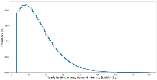
Figure 1.
Frequency of occurrence for values of yearly heating energy demand intensity.
5.3. Identify the Best DFANN Complexity
As an example, the DFANN developed specifically to assess the yearly heating energy demand intensity was used as an illustrative reference. In particular, the best DFANN complexity was identified on the basis of the following parameters:
- Number of hidden layers (Min/Max): 2/6;
- Number of nodes per layer (Min/Max): 60/280;
- Maximum number of epochs: 1000, saving the best model developed along the epochs;
- Number of DFANNs concurring with the ensemble model: 10.
The values of the loss function applied to the training and testing samples of the DFANNs are exemplified in Table 6. Conversely, the distribution of the relative errors (yPred-yTrue)⁄yTrue along the output bins is shown in Figure 2, with reference to the testing samples and to the following error intervals: error ≤ 5%, 5% < error ≤ 10%, 10% < error ≤ 20%, 20% < error ≤ 50% and 50% < error. Aside from that, the profile of the loss function value along the epochs is exemplified in Figure 3 and Table 7 (4-layer model, 280 nodes per layer), with separate references to the training and testing samples. As can be seen, the loss function curves calculated for the training and testing samples both converged to small values, therefore showing that no overfitting was taking place. Information about the input and output scaling was saved in pkl files, whereas the architecture parameters of each DFANN were saved in h5 files. Ultimately, information about the final ensemble model is represented in Figure 4 and Table 8, where the function loss values for the training and testing datasets along the epochs are shown as a whole for an ensemble model, consisting of 10 models of 4 layers and 280 nodes per layer. It is clear how the accuracy is much higher this way than in the case of a single model.
Table 6.
Examples of loss function values and training times for some DFANN architectures.
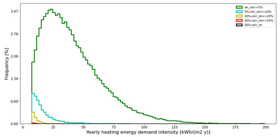
Figure 2.
Distribution of occurrence for prediction errors.
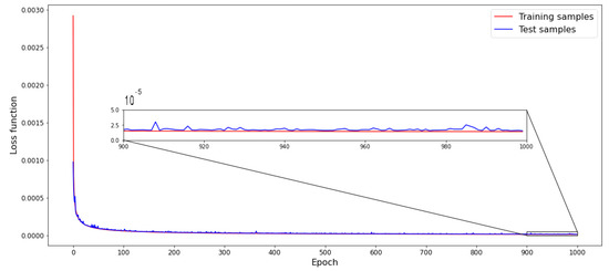
Figure 3.
Profile of function loss values for the training and test datasets along epochs for a 4-layer model with 280 nodes per layer.
Table 7.
Function loss values for the training and test datasets for a 4-layer model with 280 nodes per layer.
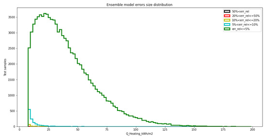
Figure 4.
Distribution of occurrence for prediction errors for an ensemble model based on 4-layer models with 280 nodes per layer.
Table 8.
Function loss values for the training and test datasets for an ensemble model based on 4-layer models with 280 nodes per layer.
6. Discussion and Further Improvements
The accuracy of DFANNs could be further improved by means of different algorithms, such as the Box Cox [43] or Yeo-Johnson [44] transformations. Since these algorithms require a normal distribution of values in order to be applied successfully, a logarithmic transformation of our values was applied so that any value distribution became quasi-normal, as is shown in Figure 5. This allowed us to take advantage of the Box Cox and Yeo-Johnson algorithms mentioned above, thus achieving even better results in a new ensemble model, which is represented in Figure 6 and Table 9. In particular, it is clear how the accuracy improved in the range of small output values, where the previous model gave higher relative errors. Obviously, the use of the logarithmic transformation involved the reverse transformation of the values coming out from the ensemble model to get the predictions back in the original scale.
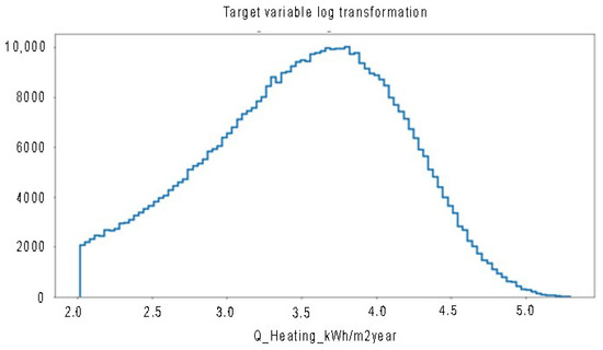
Figure 5.
Frequency of occurrence for values of yearly heating energy demand intensity after transformation of the output values into a quasi-normal distribution.
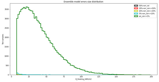
Figure 6.
Distribution of occurrence for prediction errors for an ensemble model based on 4-layer models with 280 nodes per layer after transformation of the output values into a quasi-normal distribution.
Table 9.
Function loss values on the test dataset along epochs for an ensemble model based on 4-layer models with 280 nodes per layer after transformation of the output values into a quasi-normal distribution.
6.1. Calculation Time
Finally, some considerations about the time were taken to generate predictions. A test was performed to estimate the average time taken to predict various batches of samples by means of the ensemble of 10 DFANN models described above, as is shown in Table 10. Clearly, the execution time was much shorter than only one simulation in EnergyPlus, which was about 5 s, thus making it possible to use these DFANNs for the intended application. The calculation time did not take into account the loading of scaling files and files containing models, adding up to about 3.5 s and performed just once at the program’s launch.
Table 10.
Time of execution of various batches for the ensemble of 10 models consisting of 4 layers of 280 nodes per node.
6.2. A Test on Illustrative Case Studies
Finally, the reliability of the neural networks produced was tested on a set of case studies derived from energy assessments developed by professionals. In Table 11, the main geometrical characteristics and assessed heating energy consumption of four illustrative buildings are listed. The same four buildings (buildings a, b, c, d) are also depicted in Figure 7. It was possible to verify that the neural network developed produces very reliable results. In fact, as shown in Table 11, the errors in the forecasts are very low: 3.6%, −6.87%, 4.35% and 1.69%.
Table 11.
Main geometrical characteristics and assessed heating energy consumption of four illustrative buildings.
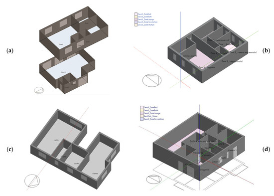
Figure 7.
Examples of buildings assessed via building energy simulation and ANNs, with (a), (b), (c) and (d) respectively referring to building codes in Table 11.
7. Conclusions
This paper deals with the generation of a set of artificial neural networks as a means to automatically assess the building energy demand from the very early design stages of a project, even in the case of interactive input/output frameworks, without the need of using any dynamic energy simulation software.
The work started from the construction of a very large database of 600,000 instances, which resulted from dynamic building energy simulations in EnergyPlus. This database was employed to train and test the set of deep feedforward artificial neural networks within an iterative process, aimed at increasing the overall accuracy of the networks. For this purpose, some additional robust techniques were also employed, such as the power transformation and ensemble approaches.
Despite the large number of input parameters, as well as their wide value ranges, the combination of these algorithms and techniques made it possible to achieve very high accuracy during the testing procedures, with errors below 5% for over 99.5% of the testing dataset, thus confirming the very high reliability and generalization capabilities of the networks.
The developed set of ANNs is therefore proposed as a reliable substitute for dynamic building energy simulation software in the design of ZEBs during the early design stages. Further steps of this work will focus on the development of similar DFANNs for building zones to allow the designer to extend the flexibility in designing complex buildings.
Author Contributions
Conceptualization, M.P., M.S., A.G.R., L.G. and L.S.; methodology, M.P., M.S. and A.G.R.; software, M.P. and M.S.; validation, M.P. and M.S.; formal analysis, M.P., M.S., A.G.R. and L.G.; investigation, M.P., M.S. and A.G.R.; resources, M.P. and M.S.; data curation, M.P., M.S. and A.G.R.; writing—original draft preparation, M.P., M.S. and A.G.R.; writing—review and editing, M.P., M.S., A.G.R. and L.G.; supervision, M.S. and L.S.; project administration, M.S.; funding acquisition, M.S. and L.S.. All authors have read and agreed to the published version of the manuscript.
Funding
This research received no external funding.
Institutional Review Board Statement
Not applicable.
Informed Consent Statement
Not applicable.
Conflicts of Interest
The authors declare no conflict of interest.
Nomenclature
| ANN | Artificial neural network |
| API | Application programming interface |
| BEM | Building energy modeling |
| BP | Backpropagation |
| DFANN | Deep feedforward artificial neural network |
| GUI | Graphical user interface |
| HVAC | Heating, ventilation and air-conditioning |
| IAQ | Indoor air quality |
| Idf | (EnergyPlus) input data file |
| PV | Photovoltaics |
| RNN | Recurrent neural network |
| ZEB | Zero-energy building |
References
- Marszal, A.J.; Heiselberg, P.; Bourrelle, J.S.; Musall, E.; Voss, K.; Sartori, I.; Napolitano, A. Zero Energy Building-A review of definitions and calculation methodologies. Energy Build. 2011, 43, 971–979. [Google Scholar] [CrossRef]
- Harvey, L.D.D. Recent Advances in Sustainable Buildings: Review of the Energy and Cost Performance of the State-of-the-Art Best Practices from Around the World. Annu. Rev. Environ. Resour. 2013, 38, 281–309. [Google Scholar] [CrossRef]
- Evins, R. A review of computational optimisation methods applied to sustainable building design. Renew. Sustain. Energy Rev. 2013, 22, 230–245. [Google Scholar] [CrossRef]
- Machairas, V.; Tsangrassoulis, A.; Axarli, K. Algorithms for optimization of building design: A review. Renew. Sustain. Energy Rev. 2014, 31, 101–112. [Google Scholar] [CrossRef]
- Li, W.; Zhou, Y.; Cetin, K.; Eom, J.; Wang, Y.; Chen, G.; Zhang, X. Modeling urban building energy use: A review of modeling approaches and procedures. Energy 2017, 141, 2445–2457. [Google Scholar] [CrossRef]
- Swan, L.G.; Ugursal, V.I. Modeling of end-use energy consumption in the residential sector: A review of modeling techniques. Renew. Sustain. Energy Rev. 2009, 13, 1819–1835. [Google Scholar] [CrossRef]
- Hirst, E.; Lin, W.; Cope, J. A residential energy use model sensitive to demographic, economic, and technological factors. Q. Rev. Econ. Financ. 1977, 17, 7–22. [Google Scholar]
- Haas, R.; Schipper, L. Residential energy demand in OECD-countries and the role of irreversible efficiency improvements. Energy Econ. 1998, 20, 421–442. [Google Scholar] [CrossRef]
- Zhang, Q. Residential energy consumption in China and its comparison with Japan, Canada, and USA. Energy Build. 2004, 36, 1217–1225. [Google Scholar] [CrossRef]
- Labanderia, X.; Labeaga, J.M.; Rodriguez, M. Policy Research A Residential Energy Demand System for Spain. Energy J. 2006, 27, 87–111. [Google Scholar]
- Summerfield, A.J.; Lowe, R.J.; Oreszczyn, T. Two models for benchmarking UK domestic delivered energy. Build. Res. Inf. 2010, 38, 12–24. [Google Scholar] [CrossRef]
- Nesbakken, R. Price sensitivity of residential energy consumption in Norway. Energy Econ. 1999, 21, 493–515. [Google Scholar] [CrossRef]
- Bentzen, J.; Engsted, T. A revival of the autoregressive distributed lag model in estimating energy demand relationships. Energy 2001, 26, 45–55. [Google Scholar] [CrossRef]
- Ozturk, H.K.; Canyurt, O.E.; Hepbasli, A.; Utlu, Z. Residential-commercial energy input estimation based on genetic algorithm (GA) approaches: An application of Turkey. Energy Build. 2004, 36, 175–183. [Google Scholar] [CrossRef]
- Saha, G.P.; Stephenson, J. A model of residential energy use in New Zealand. Energy 1980, 5, 167–175. [Google Scholar] [CrossRef]
- Fumo, N.; Rafe Biswas, M.A. Regression analysis for prediction of residential energy consumption. Renew. Sustain. Energy Rev. 2015, 47, 332–343. [Google Scholar] [CrossRef]
- Chidiac, S.E.; Catania, E.J.C.; Morofsky, E.; Foo, S. A screening methodology for implementing cost effective energy retrofit measures in Canadian office buildings. Energy Build. 2011, 43, 614–620. [Google Scholar] [CrossRef]
- Catalina, T.; Iordache, V.; Caracaleanu, B. Multiple regression model for fast prediction of the heating energy demand. Energy Build. 2013, 57, 302–312. [Google Scholar] [CrossRef]
- Amiri, S.S.; Mottahedi, M.; Asadi, S. Using multiple regression analysis to develop energy consumption indicators for commercial buildings in the U.S. Energy Build. 2015, 109, 209–216. [Google Scholar] [CrossRef]
- Parti, M.; Parti, C. The Total and Appliance-Specific Conditional Demand for Electricity in the Household Sector. Bell J. Econ. 1980, 11, 309–321. [Google Scholar] [CrossRef]
- Lafrance, G.; Perron, D. Evolution of Residential Electricity Demand by End-Use in Quebec 1979–1989: A Conditional Demand Analysis. Energy Stud. Rev. 1994, 6, 164–173. [Google Scholar] [CrossRef]
- Aydinalp-Koksal, M.; Ugursal, V.I. Comparison of neural network, conditional demand analysis, and engineering approaches for modeling end-use energy consumption in the residential sector. Appl. Energy 2008, 85, 271–296. [Google Scholar] [CrossRef]
- Matsumoto, S. How do household characteristics affect appliance usage? Application of conditional demand analysis to Japanese household data. Energy Policy 2016, 94, 214–223. [Google Scholar] [CrossRef]
- Park, D.C.; Marks, R.J.; Atlas, L.E.; Damborg, M.J. Electric load forecasting using an artificial neural network. IEEE Trans. Power Syst. 1991, 6, 442–449. [Google Scholar] [CrossRef]
- Aydinalp, M.; Ugursal, V.I.; Fung, A.S. Modeling of the appliance, lighting and space-cooling energy consumption in the residential sector using neural networks. Appl. Energy 2002, 71, 87–110. [Google Scholar] [CrossRef]
- Biswas, M.A.R.; Robinson, M.D.; Fumo, N. Prediction of residential building energy consumption: A neural network approach. Energy 2016, 117, 84–92. [Google Scholar] [CrossRef]
- Crawley, D.B.; Hand, J.W.; Kummert, M.; Griffith, B.T. Contrasting The Capabilities Of Building Energy Performance Simulation Programs. Build. Environ. 2008, 43, 661–673. [Google Scholar] [CrossRef]
- Fabbri, R.; Gabrielli, L.; Ruggeri, A.G. Interactions between restoration and financial analysis: The case of Cuneo War Wounded House. J. Cult. Herit. Manag. Sustain. Dev. 2018, 8, 145–161. [Google Scholar] [CrossRef]
- U.S. Department of Energy. EnergyPlus. 2015. Available online: www.energyplus.net (accessed on 25 May 2021).
- Klein, S.A.; Beckman, W.A.; Mitchell, J.W.; Duffie, J.A.; Duffie, N.A.; Freeman, T.L.; Mitchell, J.C.; Braun, J.E.; Evans, B.L.; Kummer, J.P.; et al. TRNSYS 16–TraNsient System Simulation Program, User Manual; Solar Energy Laboratory, University of Wisconsin-Madison: Madison, WI, USA, 2004. [Google Scholar]
- Tabatabaei Sameni, S.M.; Gaterell, M.; Montazami, A.; Ahmed, A. Overheating investigation in UK social housing flats built to the Passivhaus standard. Build. Environ. 2015, 92, 222–235. [Google Scholar] [CrossRef]
- Morgan, C.; Foster, J.A.; Poston, A.; Sharpe, T.R. Overheating in Scotland: Contributing factors in occupied homes. Build. Res. Inf. 2016. [Google Scholar] [CrossRef]
- Nowoświat, A.; Pokorska-Silva, I. The influence of thermal mass on the cooling off process of buildings. Period. Polytech. Civ. Eng. 2018, 62, 173–179. [Google Scholar] [CrossRef]
- Zinzi, M.; Pagliaro, F.; Agnoli, S.; Bisegna, F.; Iatauro, D. Assessing the overheating risks in Italian existing school buildings renovated with nZEB targets. Energy Procedia 2017, 142, 2517–2524. [Google Scholar] [CrossRef]
- Athienitis, A.; O’Brien, W. (Eds.) Modeling, Design, and Optimization of Net-Zero Energy Buildings; Ernst&Sohn: Berlin, Germany, 2015; ISBN 9783433030400. [Google Scholar]
- Østergård, T.; Jensen, R.L.; Maagaard, S.E. Building simulations supporting decision making in early design-A review. Renew. Sustain. Energy Rev. 2016, 61, 187–201. [Google Scholar] [CrossRef]
- Nord, N.; Tereshchenko, T.; Qvistgaard, L.H.; Tryggestad, I.S. Influence of occupant behavior and operation on performance of a residential Zero Emission Building in Norway. Energy Build. 2018, 159, 75–88. [Google Scholar] [CrossRef]
- Augenbroe, G. Trends in building simulation. Build. Environ. 2002, 37, 891–902. [Google Scholar] [CrossRef]
- Attia, S. State of the art of existing early design simulation tools for net zero energy buildings: A comparison of ten tools. Leed Ap 2011, 1–45. [Google Scholar] [CrossRef]
- Attia, S.; Eleftheriou, P.; Xeni, F.; Morlot, R.; Ménézo, C.; Kostopoulos, V.; Betsi, M.; Kalaitzoglou, I.; Pagliano, L.; Cellura, M.; et al. Overview and future challenges of nearly zero energy buildings (nZEB) design in Southern Europe. Energy Build. 2017, 155, 439–458. [Google Scholar] [CrossRef]
- Kalema, T.; Jhannesson, G.; Pylsy, P.; Hagengran, P. Accuracy of energy analysis of buildings: A comparison of a monthly energy balance method and simulation methods in calculating the energy consumption and the effect of thermal mass. J. Build. Phys. 2008, 32, 101–130. [Google Scholar] [CrossRef]
- ONNX. Available online: www.onnx.ai (accessed on 25 May 2021).
- Box, G.E.; Cox, D.R. An analysis of transformations revisited, rebutted. J. Am. Stat. Assoc. 1982, 77, 209–210. [Google Scholar] [CrossRef]
- Yeo, I.-K.; Johnson, R. A new family of power transformations to improve normality or symmetry. Biometrika 2000, 87, 954–959. [Google Scholar] [CrossRef]
Publisher’s Note: MDPI stays neutral with regard to jurisdictional claims in published maps and institutional affiliations. |
© 2021 by the authors. Licensee MDPI, Basel, Switzerland. This article is an open access article distributed under the terms and conditions of the Creative Commons Attribution (CC BY) license (https://creativecommons.org/licenses/by/4.0/).