Influence of Piping on On-Line Continuous Weighing of Materials inside Process Equipment: Theoretical Analysis and Experimental Verification

Abstract

Due to the continuity and complexity of chemical systems, piping and operating conditions will have a significant effect on the on-line continuous weighing of materials inside process equipment. In this paper, a mathematical model of the weighing system considering piping and operating conditions was established based on the gas–liquid continuous heat transfer weighing process. A theoretical criterion which can be extended to any continuous weighing system of the materials inside equipment with connected piping is obtained through the mechanical derivation between the material mass, the cantilever beam deflection, the strain gage deformation, and the bridge output voltage. This criterion can effectively predict the influence of piping on weighing results with specific accuracy, and provide a basis for engineering optimization design. On this basis, a set of gas–liquid continuous contact weighing devices was built. The static/dynamic experimental results showed that the accuracy of the system meets the set requirements.

1. Introduction

In chemical industry production, chemical reactions, heating, cooling, mixing, or other processes often take place in process equipment and, therefore, it must be possible to precisely measure the mass of internal materials. The total mass of the materials inside process equipment and its real-time change are important parameters, which are of great significance to the mass balance, energy balance, and device scaling-up design of chemical process [1,2,3,4]. At present, the mass measurement methods of materials inside vessels mainly include: measuring the flow of inlet and outlet, and calculating by the law of conservation of mass [5]; tracking and measuring the internal materials inside vessels using radioactive materials, and calculating according to each phase holdup and density [6]; installing the pressure sensor at the opening of the outer wall and calculating according to the pressure difference signal [7]. However, due to the complex operation state of chemical processes, the above mass measurement methods have many limitations, such as destroying the continuity of the device and operation process, large measurement error of complex phase change processes, high test cost and difficult maintenance and update, etc.

Weighing method refers to installing a weighing device directly on the equipment to obtain the total weight of the equipment and its internal materials. In the dynamic process of continuous feeding and discharging, the change of material mass inside the equipment is converted into electrical signals, and the real-time dynamic mass of the internal materials is measured [8]. As a high-precision detection method that can obtain real-time data during operation without interfering with process operation, the weighing method is not only widely used in continuous chemical production processes, but also becomes a common method to obtain process characteristic parameters in scientific research [9,10,11,12,13,14]. For example, in the fuming furnace smelting process of a nonferrous metallurgy system, the real-time mass change of pulverized coal is an important parameter in the smelting process. Weighing method obtains more reliable data than a capacitive potentiometer and other material level gauges. The dynamic mass data were obtained by on-line continuous weighing of the two-phase flow reactor, and the dynamic liquid holdup of the reactor was obtained by subtracting the dry column mass [15,16].

However, in most industrial plants there are a number of pressure vessels, or other equipment (reactors, towers, etc.), connected by a piping system used to convey fluids from one stage of the process to the next [17,18]. Evaluating the influence of attached piping on the weighing result is a bottleneck in the application of the weighing method to measure the internal material mass of equipment [19]. When the equipment moves downward under the internal material weight load, the pipe moves downward the same distance that the equipment deflects. The pipe acts like a cantilever beam, exerting a vertical force on the unit equipment. This force, together with the material weight load, acts on the weighing cell and has a significant effect on the weighing accuracy, especially when many pipes are connected to equipment with a relatively low capacity [20]. In past applications, flexible connection structures, such as PTFE pipes, corrugated expansion joints, and metal hoses, are used to minimize unwanted forces exerted by piping when the vessel deflects [21]. The angle, length, and other flexible connection parameters are demanding, but most are still based on experience. In the reaction process with phase change, high pressure will lead to the Bourdon tube effect [22], so it is necessary to fill the soft joint with flexible materials to improve its bearing capacity, but the operation is difficult. Another commonly used method to reduce the piping force is to extend the horizontal pipe section as far as possible in situations where rigid connections must be used (for example, the medium is highly toxic and highly corrosive). It is considered that the stress acting on the load cell is relatively small, and its influence on the measurement accuracy can be ignored [23,24]. In fact, any piping connections to equipment will apply some restraining force as the equipment deflects under load. The effect of piping on weight measurement cannot be completely ignored [25]. At present, there have been a lot of studies on the stress analysis of the connection between the pipe and the equipment, such as the stress analysis of the nozzle of the equipment using ANSYS [26]. However, there is neither a detailed theoretical analysis on the influence of piping forces on the material weighing results, nor the experimental data obtained by targeted experimental research.

In addition, the influence of operating pressure and material state on weighing result is another issue worthy of attention. As the chemical process is characterized by complex operating parameters and complex changes of internal materials, some studies have shown that the mass increment of gas–liquid two-phase flow under high pressure is much larger than the mass of gas-phase feeding amount, and the mass increment increases with the increase of gas velocity and pressure [27]. Therefore, it is infeasible to use the weighing method to measure liquid holdup under high pressure [28].

In order to further improve the weighing accuracy, it is necessary to quantitatively evaluate the influence of piping and operating conditions on the weighing system. In this paper, the on-line continuous weighing system of the materials inside the equipment is analyzed theoretically, so as to obtain the criterion of effective prediction of pipeline influence, which is verified by experiment. The influence of operating conditions such as pressure and flow rate on the weighing results was investigated. The results of this paper will provide a reference for the piping design of an on-line continuous materials weighing system, which is useful for the application of weighing technology in chemical processes.

2. Methodology

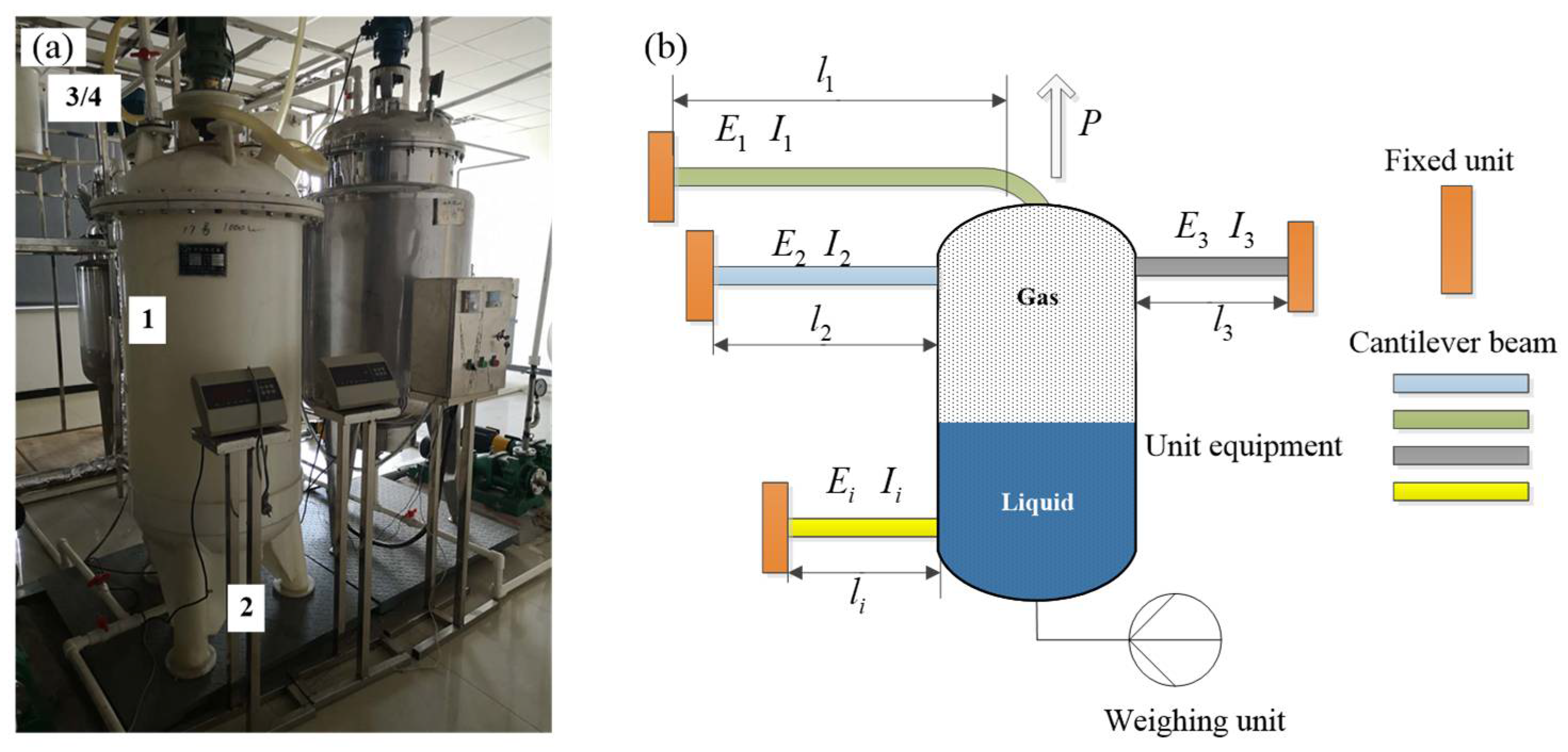
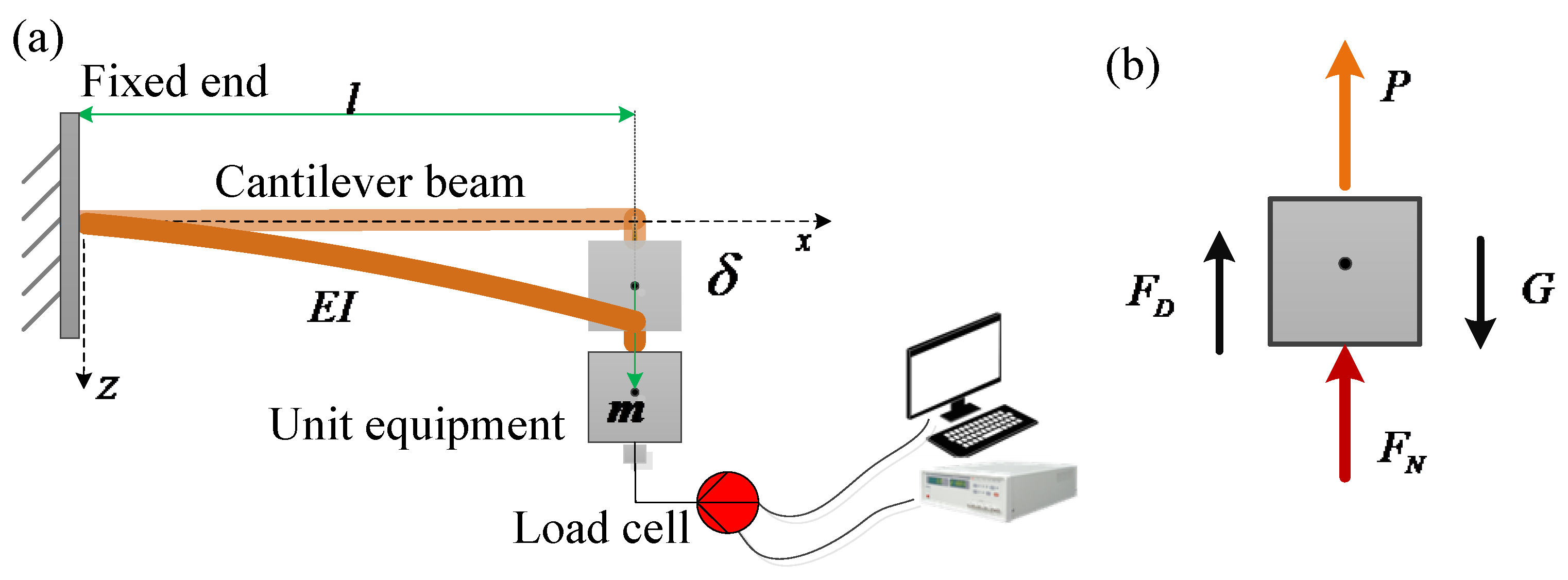
2.1. Analytical Model of the Material Weighing System inside Process Equipment

In Figure 1a, the material weighing system inside process equipment with connected piping mainly includes unit equipment with materials 1, weighing unit 2, connected piping 3, and pipe fix unit 4. Considering piping 3 is embedded to pipe fix unit 4, it can be equivalent to a cantilever beam with one end fixed. Here, pipe fix unit 4 is the fixed end, peripheral connected piping 3 is the beam [29,30]. The material mass inside the unit equipment 1 can be regarded as a concentrated load applied on the other end of the cantilever beam, as shown in Figure 1b.

Suppose that there are many cantilever beams connected to the unit equipment. Since all cantilever beams are in co-ordination with each other, the displacements at the free end are equal. With the deflection equation y = Px²(3l – x)/6EI [31], the concentrated load P_i on the end of the cantilever beam can be obtained:

$$P_i=\frac{3E_i{I}_i}{l_i^3}\delta (i\in 1,2,3,\dots \dots n)$$

(1)

where n is the number of cantilever beams, δ is the deflection of cantilever beams, E_i, I_i, and l_i represent the elastic modulus, the moment of inertia, and the length of the ith cantilever beam, respectively.

The influencing factors of temperature on beam deflection include external factors and internal factors. The external factors include ambient temperature, solar radiation, and other climatic factors. When the structure and section of the beam are fixed, the internal factors are mainly material properties, including elastic modulus and thermal parameters. Since the common external temperature range for chemical vessels is −20–200 °C, the deflection change caused by material change within this range is considered to be negligible in this study [32,33].

It can be seen from Equation (1) that the concentrated load P_i is only related to the parameters of E_i, I_i, and l_i, and has nothing to do with the position of the cantilever beams. Therefore, the multi-cantilever structure can be equivalent to a single cantilever structure, and the resultant force of the reaction force exerted by the cantilever beam on the unit equipment is:

$$P={\displaystyle \sum _{i=1}^n\frac{3E_i{I}_i}{l_i^3}\delta }=\frac{3EI}{l^3}\delta$$

(2)

where E, I, and l are the elastic modulus, the moment of inertia, and the length of the equivalent cantilever beam, respectively.

Based on the above simplification, the equivalent physical model of the material weighing system inside unit equipment with connected piping is established, as shown in Figure 2a.

For the unit equipment, an equilibrium equation of force in Figure 2b can be drawn as follows:

$$F_N+F_D+P=G$$

(3)

where F_N is the supporting force of the load cell, G is the weight of the materials and unit equipment, and F_D is the additional load generated by internal materials flow and pressure under the continuous operation condition. In the process of two-phase or multiphase flow of a chemical system, the additional load F_D represents the influence of the internal material state and the operating conditions on the mass measurement.

According to Equation (2), when the concentrated load P is applied at the end of the cantilever beam, the maximum deflection δ along the negative direction of the z-axis is generated.

$$\delta =\frac{P{l}^2}{6EI}\left(3l-l\right)=\frac{P{l}^3}{3EI}$$

(4)

Substituting Equation (4) into Equation (3), it can obtain:

$$F_N=G-F_D-P=mg-F_D-\frac{3EI}{l^3}\delta =\left(m-m_D\right)g-\frac{3EI}{l^3}\delta$$

(5)

where m is the total mass of the materials and unit equipment; since the mass of the equipment itself is constant, the change of m can be regarded as the mass change of the materials inside the equipment. The total mass m to be weighed matches the characteristics of the weighing sensor used. As long as the change of the material mass during the data collection interval is greater than the resolution of the load cell (the interval is determined by the requirements of the engineering application), the measurement can be effective. In addition, m_D is the additional mass caused by the additional load F_D.

In the weighing process, the signal of the support force F_N is converted into an output electrical signal by the load cell. For the versatility of signal acquisition, the most widely used resistance strain gauge type load cell in the industry is used.

Figure 3 is a typical resistance strain gauge load cell. It is mainly composed of an elastomer, resistance strain gauge, and bridge circuit. When a load F_N is applied to the weighing sensor, the resistance strain gauge generates strain, which is then converted into an electrical signal by the electric bridge circuit. After signal conversion, the change of the measurement value is obtained and displayed [34].

The strain of the resistance strain gauge is given as [35]:

$$\epsilon =\frac{6F_{N}L}{w{H}^2{E}_1}$$

(6)

where L, w, and H are the structural parameters of the sensor. L is the length of the cantilever of the load cell, w is the width of the beam section of the load cell, H is the height of the beam section of the load cell, and E₁ is the elastic modulus of the strain gauge material. If δ₅ is the strain of the resistance strain gauge along the direction of F_N, then there is equality δ₅ = δ. Substituting Equation (5) into Equation (6) and combining with the geometric deformation conditions, it can be deduced that:

$$\{\begin{array}{l}K\epsilon =\frac{\Delta L}{L}=\frac{\sqrt{L^2+{\delta }_5^2}-L}{L}=\frac{{\delta }_5^2}{L(\sqrt{L^2+{\delta }_5^2}+L)}\approx \frac{{\delta }^2}{2L^2}\\ K\epsilon =\frac{6KL}{w{\mathrm{H}}^2{E}_1}\left(\left(m-m_D\right)g-\frac{3EI}{l^3}\delta \right)\end{array}$$

(7)

where K is the sensitivity of the resistance strain gauge and ΔL is the absolute elongation of the strain gauge. Further derivation shows that:

$$\{\begin{array}{l}\delta =\sqrt{\mathrm{A}\left(m-m_D\right)+{\mathrm{B}}^2}-\mathrm{B} ,\\ \mathrm{A}=\frac{12K{L}^3\mathrm{g}}{w{\mathrm{H}}^2{E}_1}, \mathrm{B}=\frac{18K{L}^{3}EI}{w{\mathrm{H}}^2{E}_1{l}^3}\end{array}$$

(8)

Given that E, I, l, w, H, K, E₁, L, and g are the known parameters, A and B are regarded as given values. Hence, there is a linear power relationship between the deflection of cantilever beam δ and the mass of the unit equipment m, which is affected by the parameters of the connected beam and the load cell.

According to the bridge voltage characteristic of the load cell:

$$V_0=K\epsilon V$$

(9)

where V₀ is the output bridge voltage of the load cell and V is the supply voltage. By substituting Equations (7) and (8) into Equation (9), there is:

$$V_0=V_1-\Delta V_1-\Delta V_2$$

(10)

where:

$$V_1=\frac{6KVL\mathrm{g}}{w{\mathrm{H}}^2{E}_1}m , \Delta V_1=\frac{6KVL\mathrm{g}}{w{\mathrm{H}}^2{E}_1}{m}_D, \Delta V_2=\frac{6KVL\mathrm{g}}{w{\mathrm{H}}^2{E}_1}\frac{3EI}{g{l}^3}\delta$$

(11)

In Equation (10), V₁ is the output bridge voltage change caused by the material mass change, ΔV₂ is the output bridge voltage change caused by the internal material state and operating conditions of unit equipment, and ΔV₂ is the output bridge voltage change caused by the force of the connected piping. When there is no connected piping and the system state is stable, the voltage in the measurement system has a linear relationship with the weight to be measured.

Since the output voltage V₀ of the load cell is linearly proportional to the mass display value, if m₁ is the displayed value of the weighing indicator and the scale coefficient is k₁, then:

$$V_0=k_1{m}_1$$

(12)

Equations (11) and (12) can be combined and simplified as follows:

$$m_1=k\left(m-\Delta m\right)$$

(13)

where:

$$k=\frac{6KVL\mathrm{g}}{w{\mathrm{H}}^2{E}_1{k}_1}, \Delta m=\frac{3EI}{g{l}^3}\delta +m_D$$

(14)

Here, the coefficient k is only related to the parameters of the bridge weighing system itself, and the mass variation Δm is related to the piping parameters, the maximum deflection δ, and the additional mass m_D. Substituting Equation (8) into (13), then:

$$\{\begin{array}{l}\Delta m=\frac{2\left(m-m_D\right)}{\sqrt{\frac{2}{a^{2}b}\left(m-m_D\right)+1}+1}+m_D\approx \frac{2m}{\sqrt{\frac{2m}{a^{2}b}+1}+1}+m_D\\ a=\frac{3EI}{g{l}^3}, b=\frac{6K{L}^3\mathrm{g}}{w{\mathrm{H}}^2{E}_1}\end{array}$$

(15)

where a is the beam stiffness coefficient, and it represents the characteristic parameters of the connected piping. In addition, b is the measurement induction coefficient, which represents the characteristic parameters of the load cell.

Here, the mathematical model is performed in two typical working conditions: one is the static working condition m_D = 0, which is the non-operating working condition and there is no fluid flow and pressure inside the unit equipment; the other is the dynamic condition, m_D ≠ 0, namely the operating condition, and there is a phase flow inside the unit device and it is under a certain operating pressure.

Considering the practical measurement requirements, the model was firstly simplified under the static working conditions to obtain the parameter range of the connected piping, and the experimental verification was carried out. Then the influence of additional load on the measurement results was also evaluated through dynamic experiments.

2.2. Linearization Analysis and Evaluation Criteria

From Equations (13) and (15), it can be seen that the mathematical model of the material weighing system inside process equipment contains two parts: one is a linear term composed of mass truth value, system inherent parameters, and the additional mass m_D; the other is a power function term, which represents the measurement value variable caused by the connected piping. In order to ensure the weighing system accuracy, the value of the power function term should be controlled in a reasonable range. The relative change of the material mass caused by the connected piping is defined as the mass change coefficient m*:

$$m^{*}=\frac{\Delta m-m_D}{m}=\frac{2}{\sqrt{\frac{2}{a^{2}b}m+1}+1}$$

(16)

In engineering applications, when m* ≤ 5%, the connected piping can be regarded as a linear spring, with resistance exerted, and has little influence on the weighing result [36]. In this study, the high precision grade 1.0 of the industrial instrument is taken as a reference for theoretical analysis, which provides a basis for the accurate application of the weighing system in the following research. When m* ≤ 1%, the power function term can be ignored and the displayed value m₁ has a linear relationship with the truth value m. When m* ≥ 1%, it is considered that the influence of connected piping on weighing measurement results cannot be ignored, and the power function term should be added to the linear part to correct it appropriately.

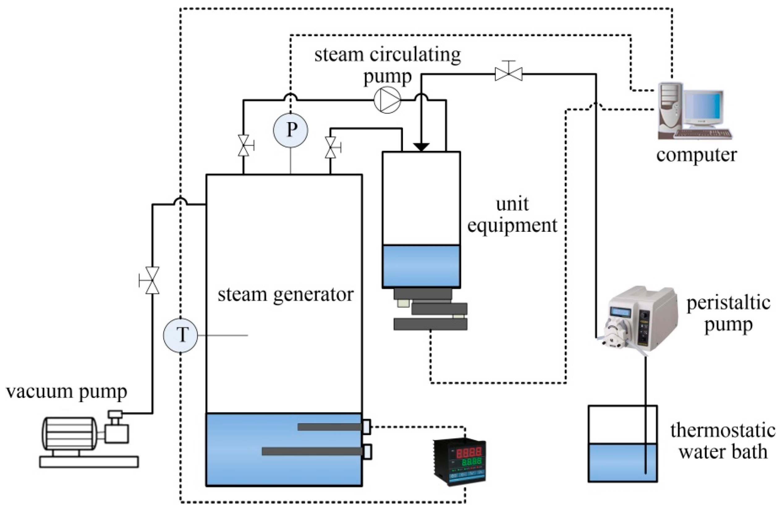
2.3. Experimental System and Conditions

As illustrated in Figure 4, the unit equipment is connected with the compression type load cell through the platform. The gas and liquid materials inside the unit equipment are provided by the low-pressure steam generation system and the thermostatic water tank, respectively, and are transported into the vessel through the piping. When the gas phase and the liquid phase contact directly, the mass transfer of the gas phase from the high pressure phase to the low partial pressure phase occurs, so that the gas phase condenses on the liquid surface. Therefore, the total amount of liquid accumulated in the container will be greater than the actual liquid inflow, and this difference is the condensation amount of steam. The real-time material mass inside the equipment is obtained through signal acquisition.

Considering the steam generator is much heavier than the unit equipment, the pipe and the steam generator can be considered as the fixed end constraint. Pressure is regulated by a vacuum pump. The vacuum degree can be up to 98 KPa. The liquid phase flows into the unit equipment from the top of the vessel. Liquid flow rate can be accurately measured by a peristaltic pump. The liquid inlet pipe adopts a flexible slender hose and is connected to the container vertically. It is considered that there is no constraint reaction force. The measurement range of the resistance strain gauge load cell is 0–1000 g, the resolution is 0.01 g, the accuracy is 0.02%, and the compensation temperature range is −10–40 °C.

The experimental study was carried out in two parts: static experiment and dynamic experiment. The static experiment was used to assess the effect of the piping and to determine the optimal parameter range. Meanwhile, the weight of materials inside the unit equipment was measured under the condition of atmospheric pressure and no flowing materials. In the process of the experiment, the material weight was calibrated repeatedly with F1 standard weight under the positive and negative stroke respectively and independently. The dynamic experiment was carried out at different pressures and liquid flows to evaluate the influence of operating conditions on weighing results. Then, the weight calibration equations were obtained by fitting the average value of the measurement results. The experimental conditions are listed in

Table 1. Experimental conditions.

Parameters	Value
Pressure/Pa	76/81/85/91/93
Steam flow rate/L∙h−1	0/0.3
Water flow rate/g∙min−1	10/20/30/40/50

.

3. Results and Discussion

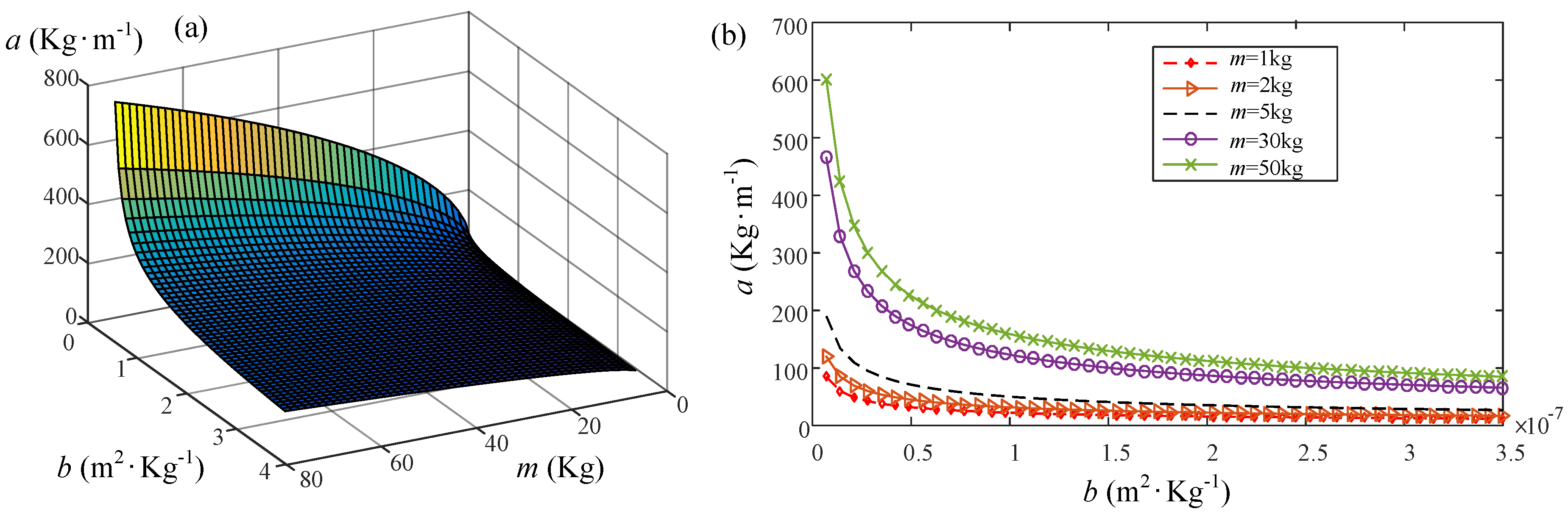
3.1. Influence Analysis of Connected Piping on Weighing Results

Figure 5a is the correlation diagram of the beam stiffness coefficient a, the measurement induction coefficient b, and the mass of the materials inside the unit equipment m, in the case of the mass change coefficient m* ≤ 1%. The diagram can provide a reference for the preliminary selection of parameters. In Figure 5b, for a certain mass m, the maximum beam stiffness coefficient of the piping decreases rapidly at first, and then basically remains unchanged with the increase of characteristic parameters of the load cell. So, the range of the beam stiffness coefficient can be defined quantitatively when the material mass or the load cell is determined. This analysis method can be applied to the engineering design of the material weighing system inside process equipment with connected piping to meet the requirements of weighing linearization.

From Equations (15) and (16), it can be seen that the characteristic parameters of the connected piping are inter-related under certain weighing accuracy. The analysis of this section can provide a basis for parameter optimization. The weighing coefficient m^c is defined as the ratio of the material mass to the measurement induction coefficient, m^c = m/b. In the project, the coefficient can be used to evaluate the mass measurement characteristics of the system synthetically. This section focuses on the relationship between connected piping parameters and the weighing coefficient m^c under specific accuracy conditions, as shown in Figure 6.

It can be seen from Figure 6 that the influence of the characteristic parameters of the connected piping decreases rapidly with the increase of the material mass initially, then slows down and eventually stabilizes. This indicates that, as the mass increases, the sensitivity of the load cell to the change of material weight is greater than the change of beam structure displacement. In the stable stage, the relative change caused by the connected piping is a constant value, and the measuring value has a linear relationship with the true value.

Figure 6a shows the correlation diagram of the elastic modulus of the materials, the moment of inertia, and the length of connected pipe in the case of the weighing coefficient m^c = 4.0 × 10¹⁰ kg²/m². The diagram can provide a basis for quantitative matching design among the characteristic parameters of the connected piping. The influence on the weighing results is small or even negligible, where the larger the elastic modulus, the longer the length or the smaller the moment of inertia of the pipe. Figure 6b shows that the influence of the elastic modulus on the mass change coefficient m* is almost proportional. As shown in Figure 6c, when the moment of inertia of the pipe is greater than 4.5 × 10³ mm⁴, the influence on m* increases gradually. When the moment of inertia is less than 1.5 × 10³ mm⁴, the value of the mass change coefficient m* ≤ 2%, it has little influence on the measurement results. However, Figure 6d indicates that the change of the pipe length has a significant effect on the weighing results. When the length is greater than 560 mm, the pipe has little influence on the weighing result, and the measurement accuracy is still within the accuracy requirement range. However, when the length of the pipe is less than 360 mm, the influence cannot be ignored.

3.2. Experiment Verification

3.2.1. Linearization Verification of Static Weighing Results

According to the linear simplification range of the mathematical model in Section 3.1, the parameters of the connected piping of the device shown in Figure 4 are determined as follows: the moment of inertia is 3.29 × 10² mm⁴, the length is 0.2 m, the elastic modulus of the materials is 127 GPa, and the total mass of the materials is in the range of 0–1000 g. The static weighing experiment was carried out and the results are shown in

Table 2. Equation and coefficient of determination (R²) between the true value m and measured value m₁.

Measurement System	Equation	R2
1	m1= 1.0161m − 1.6190	0.99999
2	m1= 1.0186m − 1.7026	0.99995
3	m1= 1.0184m − 1.5185	0.99997
4	m1= 1.0190m − 1.5840	0.99997
5	m1= 1.0188m − 1.6723	0.99997

.

The linear regression equations between the true value and the measured value were fitted. The calibration equation obtained with the average value is m₁ = 1.0181m − 1.6190, with the coefficient of determination (R²) 0.99997. The absolute maximum error, repeatability coefficient, hysteresis, and linearity of the measurement data were calculated respectively to comprehensively evaluate the absolute error, random error, and systematic error of the weighing measurement system. The results are shown in

Table 3. Absolute maximum error, repeatability, hysteresis, and linearity of measured data.

	Measurement%
Absolute maximum error	0.0012
Repeatability	0.002
Hysteresis	0.001
Linearity	0.0014

.

The maximum absolute error mainly assesses the accuracy of the measurement results, which considers the deviation in the measurement process. Repeatability is the degree of consistency of the curves obtained during multiple measurements, which is used to evaluate random errors. Hysteresis indicates the degree of noncoincidence between positive and negative characteristics during measurement. Linearity represents the degree of consistency between the input–output curve and the calibration curve. The hysteresis and linearity values reflect the magnitude of the system error [37]. The results show that the values of the four indicators are all very small, so it can be inferred that the system has high measurement accuracy and low random and systematic errors.

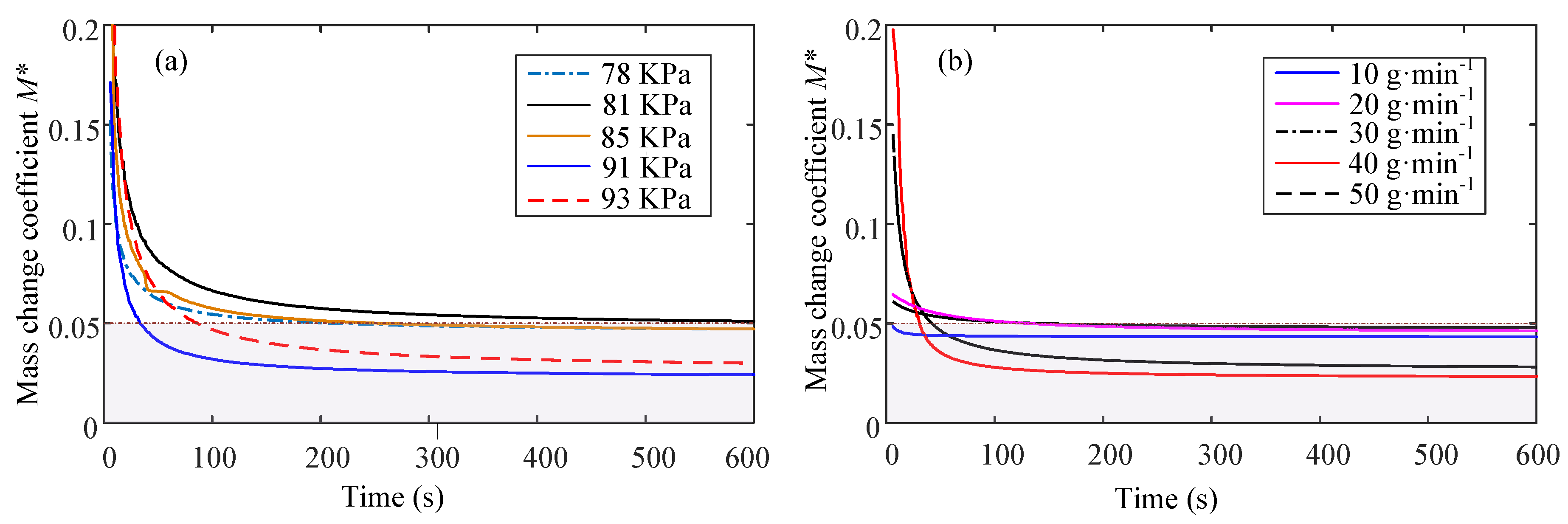
3.2.2. Influence of Operating Conditions on Dynamic Weighing

When the continuous system is in dynamic operation condition, the material flow, pressure, and other factors of the system will exert a load on the unit equipment. The exert load is superimposed on the change of the weighing measurement value and reflected as the change of the additional mass m_D in the mathematical model in Equation (16). In order to show the universality of the research, the gas–liquid reactor commonly used in the chemical production process is taken as an example. There are three main influencing factors:

• If the unit equipment is a pressure vessel, the strain generated by pressure load will be superimposed to the total strain of the system to affect the weighing measurement result;
• The gas–liquid two-phase in the flowing state inside the unit equipment can generate dynamic load and act on the internal parts of the equipment, such as the additional load;
• Harmonic load or vibration load generated by power devices and attached to the system, such as stirring device and centrifugal pump.

According to Equations (15) and (16), the relative mass change coefficient M* under dynamic working conditions is:

$$M^{*}=\frac{\Delta m}{m}=m^{*}+\frac{m_D}{m}=1-\frac{m_1}{km}$$

(17)

In order to investigate the combined influence of the connected piping and the dynamic load as a whole, the dynamic change curve of M* with time under different experimental conditions is shown in Figure 7.

The relative mass change coefficient M* drops sharply at the beginning and the value soon comes within the required accuracy range (5%), as the internal mass increases. This is because the system needs a short period of stability under the impact of the stress of connected piping and dynamic load. Finally, the combined influence of connected piping and dynamic load can be controlled within the allowable precision range. From Figure 7a,b, it can be seen that, within the same test time, the variation of the relative coefficient M* generated by liquid flow rate is more obvious than pressure, but it is still within the standard deviation. The main reason is that the liquid shock dynamic load can be reflected as the superposition of a simple harmonic displacement wave, and each specific velocity corresponds to a frequency characteristic.

In order to analyze the main reasons for data fluctuations and realize signal remolding and regression, the various frequency signals are decomposed through Fourier analysis to form waveforms with different frequencies and amplitudes [38].

As shown in Figure 8, the spectrum distributions at different flow rates are similar and the main peaks are all located at 0.2 HZ, which are inferred to be caused by the harmonic load generated by the liquid inlet device. The amplitude of the main peak of the spectrum increases obviously with the increase of the flow velocity. Therefore, the analysis results can be used as the basis for adjusting the liquid phase flow velocity. In addition, the spectrum reflects the overall vibration of the system, and the elastic coefficient of the connecting structure is far greater than the fluctuation caused by the impact load. So, the figures cannot reflect the different vibration modes of the liquid phase in a single impact on the liquid surface.

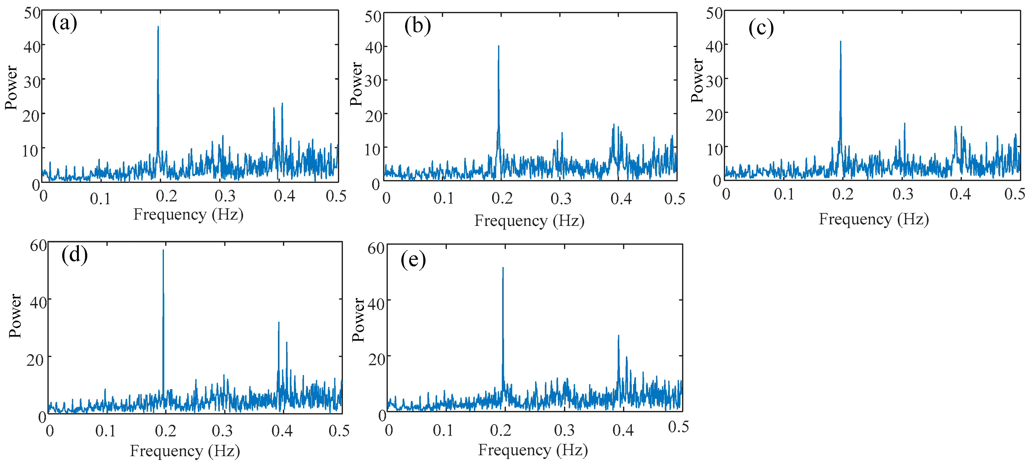
3.2.3. Linearization Verification of Dynamic Weighing Results

This section mainly investigates the characteristics of the weighing system under dynamic conditions comprehensively. The results are shown in

Table 4. Equation and coefficient of determination (R²) under different experimental conditions.

Measurement System	Equation	R2
Vacuum/kPa
76	m1 = 1.0161m − 1.6190	0.99997
81	m1 = 1.0186m − 1.6719	0.99997
85	m1 = 1.0175m − 1.5234	0.99995
91	m1 = 1.0187m − 1.6188	0.99996
93	m1 = 1.0188m − 1.7030	0.99997
Steam flow rate/L∙h−1
0	m1 = 0.9680m − 0.8627	0.99997
0.3	m1 = 0.9684m − 0.7229	0.99997
Droplet velocity/g∙min−1
10	m1 = 0.9948m − 0.3563	0.99997
20	m1 = 0.9769m − 0.3164	0.99997
30	m1 = 0.9772m − 0.5127	0.99996
40	m1 = 1.0009m − 1.1095	0.99995
50	m1 = 0.9751m − 0.6632	0.99997

.

It can be seen that the difference of experimental conditions has little effect on the linear relationship of the measured results. So the linear fitting results between the measured value and the true value of the measured mass are adaptive. The repeatability, hysteresis, and linearity values of weighing measurement data under different vacuum degrees, steam velocities, and liquid velocities are shown in

Table 5. Repeatability, hysteresis, and linearity under each experimental condition.

	Repeatability%	Hysteresis%	Linearity%
Vacuum/kPa
76	0.191	0.169	0.141
81	0.292	0.203	0.199
85	0.357	0.208	0.231
91	0.357	0.159	0.153
93	0.201	0.126	0.115
Steam flow rate/L∙h−1
0	0.353	0.270	0.286
0.3	0.410	0.269	0.284
Droplet velocity/g∙min−1
10	0.327	-	0.301
20	0.441	-	0.272
30	0.471	-	0.289
40	0.398	-	0.334
50	0.498	-	0.311

.

In the above table, the maximum value of repeatability, hysteresis, and linearity is 0.498%, 0.401%, and 0.311%, respectively, which are all reflecting the high accuracy of the system. Since repeatability is generally greater than linearity and hysteresis, it indicates that random error plays a greater role in system measurement than systematic error, which may be generated during the calibration of weights. Meanwhile, the linearity of the measured data is good with one-way change, and the value of the hysteresis error is larger than the linearity. It reflects that there is some deviation between the bidirectional and unidirectional characteristics of the system. However, for unidirectional mass change from small to large, the deviation has no significant impact on the accuracy of the system. Besides, it can be noticed that steam flow conditions have little difference in the experimental results, which indicates that the gas flow rate has little influence on the measurement results of the system. In conclusion, accurate weighing data can be obtained within the linearization range predicted by the model.

3.2.4. Uncertainty Evaluation by GUM Method

Based on the ISO GUM (guide to the expression of uncertainty in measurement) [39] uncertainty analysis system of international standards and national measurement standards, the material mass measurement inside the equipment with a connected piping uncertainty analysis method is studied. The sources of measurement uncertainty were analyzed according to the GUM method, which mainly included the standard uncertainty introduced by measurement repeatability μ_A(y). The calculations of these uncertainties are shown below.

According to Bessel’s formula, the experimental standard deviation of a single measurement is:

$$s(\alpha )=\sqrt{\frac{{\displaystyle {\sum }_{i=1}^{15}{(x_i-\stackrel{-}{x})}^2}}{n-1}}\approx 2\times {10}^{-5}$$

(18)

Therefore, the standard uncertainty component introduced by measurement repeatability is:

$${\mu }_A(\alpha )=\frac{s({\alpha }_i)}{\sqrt{5}}=8.94\times {10}^{-6}$$

(19)

The maximum permissible error of the weighing sensor is ±0.2 g, which can be converted into standard uncertainty according to uniform distribution:

$${\mu }_{B1}\left(m\right)=\frac{\sqrt{5\times (\frac{0.2}{\sqrt{3}}{)}^5}}{999.98}=1.01\times {10}^{-5}$$

(20)

The relative standard uncertainty of synthesis is:

$${\mu }_c=\sqrt{{\mu }_A(\alpha {)}^2+{\mu }_{B1}{\left(m\right)}^2}=\sqrt{{(8.94\times {10}^{-6})}^2+{(1.01\times {10}^{-5})}^2}=1.35\times {10}^{-5}$$

(21)

When k = 2, the extended uncertainty is:

$$U=k\cdot {\mu }_c=2.70\times {10}^{-5}$$

(22)

4. Conclusions

In this study, a mathematical model between the material weighing value inside unit equipment and the true value was established for a continuous gas–liquid contact weighing system with multiple pipe connections. In order to meet the specific requirements of measurement accuracy, the corresponding criteria were obtained through linearization analysis of the model, and the effects of connected piping and dynamic load on the weighing results were further studied. Finally, the theoretical analysis results were verified by static/dynamic experiments of continuous gas–liquid contact weighing. The main conclusions are summarized as follows:

(1) According to the mathematical model under static conditions, which includes the material mass, the maximum deflection of the cantilever beam, strain gauge deformation, and bridge output voltage, the linear power function relationship between the measured mass value and the truth value can be modified and simplified within a certain range. It provides a theoretical basis for improving the weighing accuracy in practical engineering application.

(2) In the required range of weighing accuracy, the quantitative relation of the beam stiffness coefficient, measurement induction coefficient, and mass of the materials inside unit equipment was obtained and provided a reference for the preliminary selection of parameters.

(3) The analysis results showed that the length of the piping has a significant effect on the weighing result, followed by the moment of inertia and the elastic modulus. Under the condition of setting the measurement accuracy, the influence of the elastic modulus on the mass change coefficient is almost proportional. Meanwhile, the moment of inertia and length can be confirmed with additional consideration of the mass measurement coefficient.

(4) Excellent linear fits were observed in the regression equations of the static experiment between the measured value and the true value, which was consistent with the linear simplification results of the theoretical model. The dynamic experimental results showed that the change of weighing value caused by operating pressure can be ignored within the operating range of this experiment. The influence of liquid velocity on weighing results was mainly reflected in the fluctuation of mass, which may be caused by the harmonic load generated by the liquid feeding device. The maximum linearity of the weighing results is 0.311%, the maximum repeatability is 0.501%, the maximum hysteresis is 0.401%, and the overall measurement accuracy meets the set requirements.

From the results of this work, theoretical analysis and experimental research are carried out on the weighing measurement of a chemical continuous system with multiple connected piping systems. Considering some problems neglected in the past, a universal mathematical model is obtained, and it provides some basis for engineering application.

References

1. Zhang, Q.; Song, H.; Liu, G.; Feng, X. Processing Unit Mass Balance-Oriented Mathematical Optimization for Hydrogen Networks. Ind. Eng. Chem. Res. 2018, 57, 3685–3698. [Google Scholar] [CrossRef]
2. Krolikowski, L.J. Distillation limit dependence on feed quality and column equipment. Chem. Eng. Res. Des. 2015, 99, 149–157. [Google Scholar] [CrossRef]
3. Suziki, I.; Yagi, H.; Komatsu, H.; Hirata, M. Calculation of Multicomponent Distillation Accompanied by a Chemical Reaction. J. Chem. Eng. Jpn. 1971, 4, 26–33. [Google Scholar] [CrossRef] [Green Version]
4. Boumans, G. Grain Handling and Storage; Elsevier: Amsterdam, The Netherlands, 1985; Volume 4, pp. 337–365. [Google Scholar]
5. Sakai, N.; Saegusa, H.; Kobayashi, M.; Tachikawa, N.; Ishikawa, I.; Mooroka, S. Development of a neutron absorption tracer technique for evaluation of fluid dynamics in coal liquefaction reactors. Fuel Process. Technol. 2002, 76, 139–156. [Google Scholar] [CrossRef]
6. Sakai, N.; Onozaki, M.; Saegusa, H.; Ishibashi, H.; Hayashi, T.; Kobayashi, M.; Tachikawa, N.; Ishikawa, I.; Mooroka, S. Fluid dynamics in coal liquefaction reactors using neutron absorption tracer technique. AlChE J. 2004, 8, 1688–1693. [Google Scholar] [CrossRef]
7. Liu, M.-Y.; Yang, Y.; Xue, J.-P.; Hu, Z.-D. Measuring Techniques for Gas-Liquid-Solid Three-phase Fluidized Bed Reactors. Chin. J. Process Eng. 2005, 5, 217–222. [Google Scholar]
8. Levec, J.; Sáez, A.E.; Carbonell, R.G. The Hydrodynamics of Trickling Flow in Packed Beds. Part II: Experimental Observations. AlChE J. 1986, 32, 369–380. [Google Scholar] [CrossRef]
9. Sbarbaro, D.; Ortega, R. Averaging level control: An approach based on mass balance. J. Process. Control 2007, 17, 621–629. [Google Scholar] [CrossRef]
10. Delgado, A.E.; Sun, D.-W. Heat and mass transfer models for predicting freezing processes—A review. J. Food Eng. 2001, 47, 157–174. [Google Scholar] [CrossRef]
11. Wiberg, P.; Sehlstedt-P, S.; Morén, T.J. Heat and Mass Ttansfer During Sapwood Drying Above the Fibre Saturation Point. Dry Technol. 2000, 18, 1647–1664. [Google Scholar] [CrossRef]
12. Mubarok, M.H.; Zarrouk, S.J.; Cater, J.E.; Mundakir, A.; Bramantyo, E.A.; Lim, Y.W. Real-time enthalpy measurement of two-phase geothermal fluid flow using load cell sensors: Field testing results. Geothermics 2021, 89, 101930. [Google Scholar] [CrossRef]
13. Fu, Y.; Xu, G.; Wen, J.; Huang, H. Thermal oxidation coking of aviation kerosene RP-3 at supercritical pressure in helical tubes. Appl. Therm. Eng. 2018, 128, 1186–1195. [Google Scholar] [CrossRef]
14. Susanti, N.; Grosshans, H. Measurement of the deposit formation during pneumatic transport of PMMA powder. Adv. Powder Technol. 2020, 31, 3597–3609. [Google Scholar] [CrossRef]
15. Holub, R.A.; Duduković, M.P.; Ramachandran, P.A. Pressure drop, liquid holdup, and flow regime transition in trickle flow. AIChE J. 1993, 39, 302–321. [Google Scholar] [CrossRef]
16. García-Serna, J.; Gallina, G.; Biasi, P.; Salmi, T. Liquid Holdup by Gravimetric Recirculation Continuous Measurement Method. Application to Trickle Bed Reactors under Pressure at Laboratory Scale. Ind. Eng. Chem. Res. 2017, 56, 13294–13300. [Google Scholar] [CrossRef]
17. Van Hessem, D.; Bosgra, O. Stochastic closed-loop model predictive control of continuous nonlinear chemical processes. J. Process. Control 2006, 16, 225–241. [Google Scholar] [CrossRef]
18. Hanakuma, Y. Present Status and Future Tasks of Nonlinear Process Modeling for Control System Design in the Chemical Process Industry. Kagaku 1998, 24, 357–364. [Google Scholar] [CrossRef] [Green Version]
19. Lakota, A. Hydrodynamics and Mass Transfer Characteristics of Trickle-Bed Reactors. Ph.D. Thesis, University of Ljubljana, Ljubljana, Slovenia, 1991. [Google Scholar]
20. Pan, J. Failure Analysis for Cracking and Deflection Deformation of Pressure Pipe-line in Synthesis Ammonia Equipment. J. Press. Vessel Technol. 2009, 26, 23–28. [Google Scholar]
21. Al-Dahhan, M.; Highfill, W. Liquid holdup measurement techniques in laboratory high pressure trickle Bed Reactors. Can. J. Chem. Eng. 1999, 77, 759–765. [Google Scholar] [CrossRef]
22. Nemec, D.; Berčič, G.; Levec, J. Gravimetric Method for the Determination of Liquid Holdup in Pressurized Trickle-Bed Reactors. Ind. Eng. Chem. Res. 2001, 40, 3418–3422. [Google Scholar] [CrossRef]
23. Crine, M.; Marchot, P. Measuring Dynamic Liquid Holdup in Trickle-Bed Reactors Under Actual Operating Conditions. Chem. Eng. Commun. 1981, 8, 365–371. [Google Scholar] [CrossRef]
24. Doihara, R.; Shimada, T.; Cheong, K.-H.; Terao, Y. Liquid low-flow calibration rig using syringe pump and weighing tank system. Flow Meas. Instrum. 2016, 50, 90–101. [Google Scholar] [CrossRef]
25. Pourmohamadian, N.; Philpott, M.; Shannon, M.A. Connection Methods for Non-Metallic, Flexible, Thin, Microchannel Heat Exchangers; Air Conditioning and Refrigeration Center, College of Engineering, University of Illinois at Urbana-Champaign: Urbana, IL, USA, 2004. [Google Scholar]
26. Costin, I.; Vasilescu, S. Pipe Stress Analysis and Equipment Nozzle Loads Evaluations. Petroleum Gas University of Ploiesti Bulletin. Technol. Ser. 2012, 64, 65–68. [Google Scholar]
27. Al-Dahhan, M.H.; Dudukovic, M.P. Pressure drop and liquid holdup in high pressure trickle-bed reactors. Chem. Eng. Sci 1994, 49, 5681–5698. [Google Scholar] [CrossRef]
28. Yang, X.L.; Euzen, J.P.; Wild, G. Study of Liquid Retention in Fixed-bed Reactors with Upward Flow of Gas and Liquid. Int. Chem. Eng. 1993, 33, 72–84. [Google Scholar]
29. Patnaik, S.N.; Hopkins, D.A. Strength of Materials; Butterworth-Heinemann: Waltham, MA, USA, 2004; pp. 129–215. [Google Scholar]
30. Megson, T. Bending of Beams. In Structural and Residual Stress Analysis by Nondestructive Methods; Elsevier: Aachen, Germany, 2019; pp. 229–279. [Google Scholar]
31. Neto, M.A.; Amaro, A.; Roseiro, L.; Cirne, J.; Leal, R. Engineering Computation of Structures: The Finite Element Method. In Engineering Computation of Structures: The Finite Element Method; Springer: Cham, Switzerland, 2015. [Google Scholar]
32. Barker, G.B. The Engineer’s Guide to Plant Layout and Piping Design for the Oil and Gas Industries; Gulf Professional Publishing: Oxford, UK, 2017; pp. 473–499. [Google Scholar]
33. Lin, X.; Zhang, Y.X.; Pathak, P. Finite element analysis of reinforced concrete beams at elevated temperatures. In Nonlinear Finite Element Analysis of Composite and Reinforced Concrete Beams; Woodhead Publishing: Cambridge, UK, 2020; pp. 83–100. [Google Scholar]
34. Fiorillo, A.; Critello, D.C.; Pullano, S. Theory, technology and applications of piezoresistive sensors: A review. Sens. Actuators A Phys. 2018, 281, 156–175. [Google Scholar] [CrossRef]
35. Watkins, K. Force, Load and Weight Sensors. In Sensor Technology Handbook; Wilson, J.S., Ed.; Elsevier: Amsterdam, The Netherlands, 2005; pp. 255–269. [Google Scholar]
36. Hős, C.; Bazsó, C.; Champneys, A. Model reduction of a direct spring-loaded pressure relief valve with upstream pipe. IMA J. Appl. Math. 2014, 80, 1009–1024. [Google Scholar] [CrossRef] [Green Version]
37. Amaral, A.M.; Filho, F.R.C.; Vellame, L.M.; Teixeira, M.B.; Soares, F.A.; dos Santos, L.N. Uncertainty of weight measuring systems applied to weighing lysimeters. Comput. Electron. Agric. 2018, 145, 208–216. [Google Scholar] [CrossRef]
38. Réti, T.; Czinege, I. Shape characterization of particles via generalized Fourier analysis. J. Microsc. 1989, 156, 15–32. [Google Scholar] [CrossRef]
39. Uncertainty of Measurement—Part 3: Guide to Expression of Uncertainty in Measurement (GUM 1995); International Organization for Standardization: Geneva, Switzerland, 2008; pp. 1–3.
Figure 1. The material weighing system inside unit equipment with connected piping: (a) physical model; (b) system diagram.
Applsci 11 05246 g001
Figure 2. Unit equipment weighing system with equivalent cantilever beam: (a) the simplified model of the system; (b) the force diagram of unit equipment.
Applsci 11 05246 g002
Figure 3. Structure of the resistance strain gauge type load cell.
Applsci 11 05246 g003
Figure 4. Schematic diagram of the weighing system.
Applsci 11 05246 g004
Figure 5. Parameter ranges under linearization condition (m* ≤ 1%): (a) characteristic parameter relationship; (b) certain mass of the unit equipment m.
Applsci 11 05246 g005
Figure 6. Influence of connected piping parameters on the mass change coefficient: (a) characteristic parameter relationship; (b) materials; (c) moment of inertia; (d) length.
Applsci 11 05246 g006
Figure 7. Influence of dynamic working conditions on the relative mass change coefficient M*: (a) pressure; (b) liquid flow rate.
Applsci 11 05246 g007
Figure 8. FFT transform results of transient mass signals at different liquid flow rates: (a) 10/g∙min−1; (b) 20/g∙min−1; (c) 30/g∙min−1; (d) 40/g∙min−1; (e) 50/g∙min−1.
Applsci 11 05246 g008