1. Introduction
Landslides are one of the world’s major geohazards that threaten exposed areas both in urban and rural areas and cause severe consequences shown in lost human lives as well as economic losses. Due to the climate change, there is an increase in frequency and intensity of heavy rainfall along with shift of locations and recurrence of rainfall which significantly increases landslide risk in landslide prone areas. Expansion of urban areas due to population growth, developments in mountain and coastal areas, including construction of roads and railways, and deforestation increase exposure to the landslide hazard [
1].
Because of severity of the landslide hazard, many scientists and engineers work to develop the landslide science and reduce the landslide risk. One of the fields of the landslide science is landslide modeling, which gives an opportunity to explore landslide triggers and landslide process evolution. For a long time, landslide modeling was based only on numerical modeling techniques. Physical modeling of landslides using scaled landslides models behavior started in the 1970s and 1980s in Japan on natural slopes exposed to artificial rainfall [
2,
3,
4,
5]. In the field, large-scale experiments of debris flows were performed in the 1990s in USA [
6,
7]. Laboratory experiments of landslide behavior in a scaled physical model (also known as flume or flume test) started in the 1980s and 1990s in Canada [
8], Japan [
4], and Australia [
9] under 1 g conditions. In the following years, the main purpose of landslide physical modeling was research of initiation, motion, and accumulation of fast flow-like landslides caused by infiltration of water in a slope and fluidization [
10,
11,
12,
13,
14,
15,
16]. Research of physical models can be divided in two main groups in relation to main landslide triggering factors: rainfall and earthquakes.
Physical models used for simulation of landslide initiation and motion triggered by rainfall infiltration were utilized for identification of rainfall threshold for landslide initiation [
17,
18,
19]; infiltration and seepage-induced landslides [
20,
21,
22,
23]; and deformation and failure characteristics of soil in a slope [
24,
25,
26]. The physical models are also very useful for modeling unsaturated soil behavior in slopes where landslides occur in partially saturated to saturated conditions. The main aim of those models was rainfall infiltration in unsaturated soil in a slope and landslide initiation [
27,
28,
29,
30].
Landslide modeling on a small scale has found a wide application in analyzing different types of landslides (e.g., flows, slides, falls, and topples) in different materials (sandy, silty, and clayey material) and with different boundary conditions and abilitoes to analyze whole spectrum of mechanisms and processes. In October 2018, the Faculty of Civil Engineering, University of Rijeka, Croatia, started a research project “Physical modeling of landslide remediation constructions’ behavior under static and seismic actions”, funded by the Croatian Science Foundation. The purpose of this paper is focused on only static conditions in landslide triggering, i.e., rainfall-triggered landslides.
The slope model was built of sandy material built-in under different inclinations, and a failure was triggered by an artificial rainfall. The main focus of this research was to present abilities of monitoring landslide development by combining geotechnical monitoring equipment with noncontact optical measurements. The results of the small-scale landslide development were observed by monitoring the surface changes with high-speed cameras, terrestrial laser scanner, and structure-from-motion (SfM) photogrammetry method as well as by monitoring of pore water pressure and displacements inside the sliding mass. Beside the methods and types of the monitoring equipment acquired and used in these experiments, physical properties of the soil material in the slope, the methods of constructing the small-scale flume and some of the results obtained from the tests are also presented in this manuscript. The test results contribute to the improvement of the monitoring system and selected measuring equipment both in future tests of the project as well as similar type of research in small-scale physical modeling.
2. Physical Model
The physical model of a scaled slope was designed to enable initiation of a landslide caused by controlled artificial rainfall and equipped with adequate photogrammetric equipment and complex sensor network with the ability to measure displacements, soil moisture, pore pressures, and suction within a landslide body (
Figure 1a) [
31,
32,
33]. The flume lies on the working platform and is constructed of a steel base plate with transparent plexiglass sides to enable observation of the wetting front and the development of cracks during the test (
Figure 1b). Dimensions of the flume are as follows: 1.0 m (width) × 2.3 m (length) × 0.5 m (height). In relation to the slope dimensions, the maximum depth of the soil material in the slope was adopted to be 30 cm. Flume slope inclination can be adjusted for a certain type of used soil material from 20
to 45
. To prevent possible sliding of the soil mass at the contact with the flume base, the geogrid mesh is fixed to the flume base to increase friction. The series of tests were conducted at different slope inclinations of 30
, 35
, and 40
degrees.
2.1. Soil Material Properties and Preparation of the Model
Due to the relatively simple behavior of the infiltration process and the failure triggering, the fine (0–1.0 mm) sandy material was chosen for the initial test series. The grain size distribution of the selected Drava River sand is presented in
Figure 2, while
Table 1 presents its basic physical properties and initial conditions at the start of the tests. Friction angle and cohesion were determined in direct shear apparatus at the same relative density of 50% and at low normal stresses similar to those present in the slope model. Hydraulic conductivity at same conditions as in the slope model was determined by falling head test in oedometer.
The previously described Drava River sand was built-in in the flume in five layers each 6 cm thick, to the total height of 30 cm. Pre-prepared sandy material at water content of
was built-in using the under compaction method [
34]. Each layer was compacted by the manual compactor to the medium dense conditions of relative density
. Before the placing of a next layer, the previous ones’ surface was raked and sprayed with water in order to maintain the initial moisture and to achieve the best possible connection between particles of each layer. To reach homogeneity of the material in the slope and relatively uniform conditions in built-up sandy material, the model was built in three segments—lower (L), middle (M), and upper (U) part—building up the material from the foot to the top of the slope. The details of the build-up layer dimensions and properties are presented in
Table 2.
2.2. Rainfall Simulator
One of the most important issues in the physical models that simulate landslide initiation and motion caused by rainfall infiltration is a full control of the intensities of artificial rainfall applied to slope models. Rainfall simulators are a widespread tool for studying hydrologic processes such as the interaction of rainfall with soil, soil erosion, surface runoff, and infiltration [
35]. Although it was possible to use already-developed rainfall simulators [
35,
36,
37], due to the lack of standard designs and necessity to develop a rainfall simulator adjusted for rainfall intensities characteristic for the precipitation events in Croatia, the rainfall simulator was constructed inside the project. The idea was to develop a rainfall simulator that could be used on a wide spectrum of soil materials from sand to silt and clay. As each material has a very different hydraulic conductivity and ability to infiltrate different amounts of water in the same period, a simulator that can cover all soil types had to be designed in adequate scale ratio. The artificial rainfall also should have sufficient spatial uniformity. Rainfall simulator system was constructed of three sprinkler branches, each branch consisted of four different axial-flow full-cone nozzles with spray angle of 60
. Each branch was placed at such a height as to allow water to reach the edges of the plexiglass sides without creating too much water at the edges or water coming out of the model. This solution covers a wide range of rainfall intensities, from below than 30 L/h/m
2 to above than 140 L/h/m
2 at the reference pressure of 2 bar. Wide range of rainfall intensities and possibility of changing location of rainfall by switching branches on/off gives the ability to model different rainfall patterns and different rainfall intensities applied to the slope model.
3. Review of Landslide Monitoring Equipment
By definition, a movement is a term that characterizes landslides [
38]. That is why a movement distribution along a slope is the most important data for all landslide analyses [
39] and presents an important object of landslide monitoring. According to Savvaidis [
40], the types of monitoring systems and techniques can be divided into groups as follows: (i) remote sensing or satellite techniques; (ii) photogrammetric techniques; (iii) ground-based geodetic techniques; (iv) satellite-based geodetic techniques; and (v) geotechnical techniques. Selection of instrumentation and methods for landslide monitoring system largely depends on movement types and deformation as well as the purpose of the monitoring campaign [
40]. Monitoring system should be suitably designed for the type of experiment being performed, and equipment installed at the correct locations to take into account the possible positions of the sliding zone. Monitoring system established in a physical model follows the principles used in observation of real landslides, and it consists of a geodetic monitoring system and geotechnical monitoring system [
39]. Design of the monitoring system greatly depends on the experience of the users and the needs of the experiment. Although most of the equipment is miniature in a size comparison with in situ equipment for landslides, it depends on the projected size of the flume model. In
Table 3, the summary and purpose of equipment used in small-scale physical models are provided along with a literature review.
3.1. Geodetic Monitoring System in Small-Scale Landslide Modeling
Geodetic monitoring system is based on innovative photogrammetric equipment for multitemporal landslide analysis [
51] of image sequences obtained by a pair of high-speed stereo cameras [
41]. Terrestrial laser scanner and structure-from-motion (SfM) photogrammetry surveys enabled determination of the surface of the slope model in the stages before and after the sliding [
52].
3.1.1. High-Speed Cameras
High-speed cameras used for multitemporal landslide analysis from stereo image sequences are part of the ARAMIS system (GOM GmbH, a ZEISS company, Braunschweig, Germany) [
53]. ARAMIS is an optical noncontact 3D measuring system by the German company GOM that provides the whole workflow from conducting the measurements, through the analysis of measurement obtained raw data and to the representation of the results. Camera frequency options depend on used sensor or cameras: a single camera system can determine 2D coordinates and measure flat objects, while a stereo pair of cameras system can determine 3D coordinates and measure position of objects in 3D. The software computes coordinates in 3D space and assigns points from the camera images to each other. To be able to compute 3D coordinates, a software needs reference points. Reference points can be point patterns or random patterns which are also called stochastic patterns. Reference point patterns consist of self-adhesive circular points markers with a black background and white center to act as a contrast between black and white color in the software identification along with the orientation of the reference marker points. Random reference patterns can be applied with spray cans or a brush. Over a period of time, the system monitors 3D coordinates. Software then compares coordinates computed during the measuring sequence to derive displacement of the pattern marks to each other [
53]. By using the principle of triangulation, software uses computed image point coordinates to compute 3D points on a surface. The point of origin can be calculated if the software recognizes at least two or more signals coming from a point. Software recognizes light by using optical sensors and information from the sensor calibration for the characteristic measured volume and determines spatial coordinates of origin. For the triangulation to be as precise as possible, it is necessary to consider intrinsic or internal camera parameters and extrinsic or external camera parameters. Intrinsic parameters depend on the type of camera used and are internal specifications of the camera, and they are parameters needed to describe the orientation in the image plane. Extrinsic parameters are related to the orientation in space and the position of the camera in the global coordinate system [
54].
The ARAMIS system sensors enable real-time measurement for a large number of points on the surface of an observed object. The system is adjustable, meaning it can measure a wide range of volumes—from samples of a few square millimeters to few square meters. The flexibility of sensor use due to the variable measuring volumes and distances facilitates variety of measuring tasks. Optical measuring system consists of a sensor with two cameras (3D setup), cables, stand, calibration object, pair of lenses, laser pointer for optimum sensor adjustment, LED lights, and a photocell.
The series of tests was recorded by the above-described set of two 4-megapixel cameras. In the later stages of the project, another set of cameras was obtained. This system works on the same principle but with a few improvements—two 12-megapixel cameras with high spatial resolution and a pixel size of 3.45
m [
55]. In
Figure 3, both sets of cameras are shown, while in
Table 4, characteristics of both camera systems are stated for comparison.
The first image sequence made of the measuring object presents the initial state of the object before the test. Before the beginning of the test, an initial calibration dependent of the measuring volume must be conducted. For the small-scale landslide physical model, a calibration cross (2 m dimensions) for bigger volumes was used. ARAMIS system was not used before in similar research to observe surface displacements in a landslide body, but it was used and checked in several different dynamic experiments in observation of surface point displacement and velocity measurements [
56,
57].
3.1.2. Terrestrial Laser Scanner (TLS) and Structure-from-Motion (SfM) Photogrammetry
Terrestrial laser scanner (TLS) used to capture model surface is the FARO Focus 3D X 130 (FARO Technologies Inc., Lake Mary, FL, USA) shown in
Figure 4a. Similar laser scanner, a Leica ScanStation 2, was used by Wu et al. [
44] in laboratory experiments to capture deformation of loess slope surface. FARO Focus 3D X 130 is a high-speed three-dimensional terrestrial laser scanner for detailed measurement and documentation. Single-point measurements are repeated up to 976,000 points in a second; therefore, the resulting images are an accumulation of millions of 3D measurement points. Main features of the laser scanner are: high accuracy, high resolution, high speed, intuitive control via the built-in touchscreen display, high mobility due to its small size, light weight and integrated quick charge battery, WLAN for remote control, integrated dual axis compensator to automatically level the captured scan data, integrated GPS sensor to determine the position of the scanner, integrated compass and altimeter for orientation and height information of the scans, and 3D color scans because of the integrated color camera with a resolution of 70 megapixel. Technical specifications of the laser scanner are stated in
Table 5 [
58].
The Focus TLS works by sending an infrared laser beam into the center of its rotating mirror. The mirror deflects the laser beam on a vertical rotation around the environment being scanned; scattered light from surrounding objects is then reflected back into the scanner. Scanner uses phase-shift technology to measure distance where constant waves of infrared light of varying length are projected outward from the scanner. Upon contact with an object, they are reflected back to the scanner. The distance from the scanner to the object is accurately determined by measuring the phase shifts in the waves of the infrared light. The
x,
y, and
z coordinates of each point are then calculated by using angle encoders to measure mirror rotation and the horizontal rotation. These angles are encoded simultaneously with the distance measurement. Distance, vertical angle, and horizontal angle make up a polar coordinate (
), which is then transformed to Cartesian coordinates (
x,
y,
z). The scanner covers a 360
× 300
field of view (horizontal × vertical) [
58].
The laser scanner does the measurement in two steps: first one being the measurement of geometry and defining of x, y, and z coordinates, and the second one is the photographing process for determination of colors. Colors are determined by the red/green/blue (RGB) scheme where each pixel consists of a certain combination of red, green, and blue light (from 0 to 255) which in return give a certain color depending on the strength of each color. Scans can be conducted in color or monochromatic, which visually gives better information about the geometry itself because of the use of different shades of grey. The amount of light determines the intensity of the color, and after monochromatic measurements, there is spherical photographing which allows for a scan in color.
References or targets are used to achieve the overlap of multiple individual scans, each with their own coordinate system, onto a single scan with aligned coordinate system. Different targets can be used as an artificial reference object, such as checkerboard paper targets or reference spheres which were used in this test (
Figure 4b). Target spheres should be spaced as far apart as possible but within the overlapping scan areas. Higher number of references per scan may improve scan results and make the registration easier and less prone to errors [
58]. If correctly positioned, the laser can see reference spheres in all conditions. It defines the center of the sphere, connects them over all the scans, and defines the relative coordinate system.
SfM allows for the creation of 3D models from multiple overlapping images taken at distinct triangulation angles. Lighting differences usually cause problems while processing data, but many types of software have the ability to estimate potential errors and delete images whose accuracy is questionable [
59]. The method works by analyzing whole images, searching sectors with similar pixels in all the taken images, and triangulating the position of the camera.
SfM photogrammetry survey of the physical model was carried out only for the first test in the series by a Nikon D500 camera with an ultrawide angle lens Tokina AT-X 11–20, which allowed the determination of a 3D landslide surface model similar to that obtained by a laser scanner.
3.2. Geotechnical Monitoring System
Geotechnical monitoring system is comprised of a complex network of miniature sensors equivalent to in-field used geotechnical monitoring equipment [
60]. Various researchers established different monitoring systems using available sensor types for small-scale models [
42,
43,
46,
47,
48,
49] with a wide range of abilities—measuring soil moisture, pore pressure, displacement, suction, etc. All sensors used in the tests are constantly connected to data loggers for continuous data collection during the time of the test.
3.2.1. Water-Related Sensors
All water-related sensors are from the manufacturer METER Group (METER Group AG, München, Germany), including the two data loggers we have obtained specifically for collection of data from these sensors. Data loggers are METERS’ ZL6 six-channel loggers with integrated GPS and ZENTRA application which can be accessed from tablets or smartphones. METER data loggers have sensor logging interval from 5 min to 12 h and can return the average or accumulation of the one-minute sensor readings across a chosen measurement interval. All of the sensors from the METER Group have low power requirements, which is ideal for long-term experiments on soils in laboratory or in the field.
Soil moisture sensors are called TEROS 10 and TEROS 12. TEROS 10 series are simpler, low-cost sensors that measure volumetric water content (VWC), while TEROS 12 series additionally has the ability to measure temperature and electrical conductivity of soil. Both types of sensors use an electromagnetic field to measure apparent dielectric activity (ε
a). Frequency capacitance technology is used to supply a 70 MHz oscillating wave to the needles; the difference being that TEROS 10 only has two stainless-steel needles and TEROS 12 has three stainless-steel needles (
Figure 5). Needles charge according to the dielectric of the material, and charge time is proportional to substrate dielectric and substrate VWC. Charge time is measured and outputs raw value based on the substrate ε
a, which is then converted to VWC by a calibration equation [
61,
62].
While installing the sensors, it is necessary to avoid installation near large metal objects that can affect their function and distort readings. If the sensor is installed in a vertical position, more soil depth is integrated in the soil moisture measurement. In horizontal installation, the sensor provides soil moisture measures at more discreet depths. Ferrite core on the sensor cable works as an isolation from interferences and potential noises from the system; therefore, this section of the cable from the sensor to the core should not have anything attached [
61,
62].
In addition to VWC and temperature measurements, TEROS 12 monitors electric conductivity (EC). Soil moisture (VWC) is measured between needle 1 and needle 2 and electric conductivity between needle 2 and needle 3. Embedded thermistor located in the central needle takes temperature readings and responds faster to temperature changes than its similar sensor TEROS 11, which is without EC measurements. Output temperature is in degrees Celsius, unless otherwise stated in the data logger program [
61,
62]. Another advantage of the TEROS 12 sensors is their measurement volume of 1010 mL, which is a big volume for the size of the sensor. In
Table 6, ranges of volumetric water content, temperature, and electric conductivity are stated.
The soil water potential sensor that is used in the model is TEROS 21, although it is not considered as a standard tensiometer sensor due to the lack of ability to measure positive pore pressure. All soil water potential measurement techniques measure the potential energy of water in equilibrium with water in the soil in accordance with the Second Law of Thermodynamics. After coming into hydraulic contact with the soil, the sensor water potential comes into equilibrium with the water potential of the soil [
63].
TEROS 21 sensors measure the water potential and temperature of soil with two porous ceramic discs (
Figure 5). The sensor measures moisture changes of ceramic discs sandwiched between stainless-steel screen and the circuit board. By introducing a material with known pore size distribution and achieving equilibrium with the soil, soil water potential can be measured. TEROS 21 measures dielectric permittivity of a solid matrix (porous ceramic discs) to determine its water potential. Using the moisture characteristic curve of the ceramic, the water potential can be derived from the readings of the water content. For accurate measurements, a good hydraulic contact with the surrounding soil must be achieved during the sensor installation. While TEROS 21 does not have the accuracy of tensiometers and the ability to measure positive pressure, its extended range for negative pressure, i.e., matric suction, that can be seen in
Table 6, makes it an ideal sensor for dry soils and high matric suction (e.g., clays) where tensiometers have a cavitation problem [
63].
Although there are many studies which used similar types of sensors to monitor volumetric water content and soil potential from different manufacturers, the most important are studies from Huang and Lo [
23] and Wu et al. [
44], as their sensors are predecessors of the TEROS sensors. The reliability and accuracy of the sensors is defined by the manufacturer and can be checked with an accuracy verification standard. For a simple material like sandy soil, generic calibration curve for all soil types was used, which ensures accuracy of
3% of sensor readings.
3.2.2. MEMS Accelerometers
Sensors used for observations of acceleration in the model are micro-electro-mechanical systems (MEMS) that are made using the techniques of microfabrication and have miniaturized mechanical and electromechanical elements. Two different types of MEMS accelerometers were used in the tests—ADXL345 by ANALOG DEVICES (Analog Devices Inc., Wilmington, MA, USA) and MXR9150M by MEMSIC (MEMSIC Inc., Tianjin, China), which are shown in
Figure 6 and their specifications compared below in
Table 7. Production and development of MEMS sensors is very broad with different base designs; therefore, comparisons between similar sensors are hard to make, but Ooi et al. [
19,
47], Wang et al. [
48], and Ooi and Wang [
49] used similar types of ADXL sensor by ANALOG DEVICES. Results from the MEMS sensors also depend on the operators’ method of calibration, sensor bias (offset), and sensitivity of each sensor type.
The ADXL345 MEMS is a 3-axis digital accelerometer with high-resolution (13-bit) and measurement ability up to
. It is supplied in a small, thin LGA package with dimensions of 3 × 5 × 1 mm. Sensor has low power dissipation due to intelligent motion-based power management where power is 0.1
in standby mode and 23
in measurement mode at typical power supply of 2.5 V. It can measure both dynamic accelerations resulting from motion or shock and static acceleration, such as gravity, which allows it to be used as a tilt sensor. ADXL345 has free-fall detection,
shock survival, wide operating temperature from
to
, and a very small device weight of 30 mg. Because of its high resolution, it can measure inclination changes smaller than 1.0
[
64].
The sensor consists of polysilicon surface-micromachined structure that is built on top of a silicon wafer. Springs suspend the structure over the wafer and provide a resistance to forces from the acceleration. The shift in the structure is measured using differential capacitors that consist of fixed plates and plates attached to the moving mass. Acceleration causes a shift of the proof mass and unbalances the differential capacitor which results in a sensor output amplitude proportional to acceleration [
64].
The MXR9150M MEMS is a low-cost 3-axis analog accelerometer with measurement ability up to . It is supplied in a hermetically sealed, surface mount LCC package with dimensions of 7 × 7 × 1.8 mm. It can measure both dynamic acceleration and static acceleration such as gravity. Operating temperature is in a wide range from to and has a shock survival rating .
Unlike the ADXL345, the MXR9150M MEMS is a thermal accelerometer designed based on heat convection and does not require proof mass to function, which gives it such a big shock survival rating. This MEMSIC sensor operates like other accelerometers with proof mass except it is a gas in the sensor. In the center of the silicon chip is a heat source, suspended across a cavity with four equally distanced aluminum/polysilicon thermopiles on all four sides of the heat source. Temperature gradient is symmetrical about the heat source, if no acceleration is applied, temperature is the same in each thermopile, and consequently, they all output the same voltage. Acceleration causes a disturbance in the temperature profile which becomes asymmetrical. Since the temperature of the four thermopiles is different, voltage output is also different. Voltage at thermopile outputs is directly proportional to the acceleration [
65].
4. Results
After the construction of the slope model and installation of the monitoring equipment in a slope, a slope model was exposed to the artificial rainfall from three nozzles, one nozzle in each part of the slope—upper, middle, and lower part. Inclination of slope, duration of tests, and intensities of rainfall are listed in
Table 8.
4.1. High-Speed Cameras
The results of high-speed camera measurements are 3D coordinates captured in time and derived calculated values such as displacements, strains, velocities, and accelerations at individual points on a landslide surface caused by static or dynamic loads. The principle of measurement is based on digital image correlation and successfully replaces a large number of traditional measuring devices (e.g., LVDTs, strain gauges, extensometers, and accelerometers).
A small-scale physical model of landslide constructed in the laboratory was observed by a pair of high-speed cameras to obtain stereo pair image sequences (
Figure 7a,b) used for multitemporal landslide analysis. The duration and changes in filming frequency during the tests conduction are listed in
Table 9.
In the following text, the results obtained in the Test 2 are described together with an analysis of the surface displacement. The whole Test 2 was recorded in 479 image sequences according to the filming duration of 2 h 11 min 10 s. As there is almost no change in displacement in the beginning of the test, recording speed was adjusted in several stages of the recording, becoming increasingly dense at the end of the test when most of the displacements happened.
Reference points used on the physical model were circular white pins dyed with black marker; therefore, the reference is based on the contrast of black and white. Pins are arranged in the regular mesh at the distances of 20 × 10 cm, in 5 rows and 24 columns from the camera view, with total number of 120 reference pins. The analysis along the middle longitudinal profile of the slope model is presented here. The next few figures show the process of analysis of displacements and deformations of the surface of the physical model along the profile. Because of a large number of the recorded image sequences, there are too many graphical stages to be presented, which is a reason why only points along one profile are analyzed and shown. Point markers are named by their position: the first number in the name represents the row, and the second number represents the column of the marked point, as is shown in
Figure 8. To be able to track a point through the recording, the point must be visible at all stages in both cameras. Every point marker within the field of view is assigned values of
x,
y, and
z coordinates based on the recognized reference point. Certain points are not assigned because they are not visible in both sets of images (e.g., the first column at the bottom of the model was not considered because the left camera did not encompass that part of the landslide model). Additionally, some points could not be assigned due to the elements of the platform that cover them, such as constraints of plexiglass sides and tensioned wire stretched over the model.
Observed points are linked by lines in a longitudinal profile made of points from the second row (
Figure 9). Connecting the points in lines allows for easier follow-up in the next stages of the test. This profile is one of the best examples because almost all points from the second row are visible in the undeformed reference stage (Stage 1) shown in
Figure 9. Point 2,1 was not recorded by the left camera, and point 2,7 was not visible due to the tensioned wire placed just above the point in the lower part of the model as a protection from buckling of the plexiglass sides.
Changes of
x,
y, and
z coordinates, i.e., displacements, are measured by comparison with the position of the recognized reference points through consecutive images that correspond to different degrees of deformation (stages through time). Since the whole test was recorded in the sequence of 479 images, a few characteristic stages of the recorded test were chosen and presented for the visible points. Besides the initial stage (Stage 1), two other stages were chosen because of the visibility of points and the biggest displacements happening around that time—stage 330 and stage 434. Comparing the reference undeformed image from stage 1 to stage 330 visible in
Figure 10 which was recorded at the moment of formation of the crack at the bottom of the middle part of the model, on the edge of the point 13. Here, all points before number 13 are lost in the sliding of the mass or covered by the water level that formed at the foot of the slope. Further, points 15 and 16 are not visible above, probably due to the poor lighting and creation of a shadow above the aforementioned points. At the top of the model, on the horizontal part of the line, point 23 cannot be defined. The possible reason could be the reduced visibility of the point by retaining water droplets on it and/or the position of the point being too close to the plexiglass.
In Stage 434 (
Figure 11), other points above the point 13 are lost in the sliding of the material and separation of the inclined part of the slope from the upper horizontal part of the slope. However, here, by comparing the values of
x,
y, and
z coordinates of the few visible points such as 19, 20, and 21, the subsidence of material is noticeable in those points due to the formation of cracks inside the landslide body. By further retrogressive movement of the slope, the marker points slide along with the material, and the system cannot recognize points covered by the material or submerged in water; therefore, the visibility of an increasing number of points decreases through stages of the test.
The changes in the longitudinal profile during the test can be graphically presented as in
Figure 12. It can be possible to monitor the movements of the observed marker points along the profile and compare the stages with the soil moisture contents. For example, Stage 330 (
Figure 10) is immediately after the landslide initiation when the constant VWCs were reached at all sensor depths, landslide development was retrogressively developed, and the disturbance in the middle part of the slope at the shallowest sensor at the depth of 6cm was identified. In
Figure 12b (Stage 360), points 15 and 16 are lost probably due to the poor lighting or shadow fell at the points, while in
Figure 12c, only the upper part of the profile is visible as the material of the slope just subsided and has not flown downward yet.
4.2. Terrestrial Laser Scanner (TLS) and Structure-from-Motion Photogrammetry
The scan of the small-scale landslide physical model consists of approximately 5–6 individual scans made from different positions around the model, each scan with up to 7 million points and approximate scan duration of 5:30 min. After the first scan which was made in color, scans for other two tests were monochromatic as they proved to provide better visualization of geometry due to the use of different shades of grey. Distance of the scanner from the object was from minimal 0.8 m to maximal 2 m. Initial processing and registration was performed in the FARO SCENE software. Merging of scans into a single point cloud and reduction of unnecessary number of points by a minimum distance of 1 mm performed in CloudCompare software [
67]. The most important settings of the laser scanner used for the recording of the tests are stated below in
Table 10.
The resulting 3D point clouds before and after the sliding in Test 3 are presented in
Figure 13a,b, respectively.
Figure 13c is a photograph taken of the physical model at the end of the test, and in
Figure 13d, cross-sections of the central longitudinal profile along the slope can be observed. The green dotted line presents the profile before the sliding, and the blue full line presents the profile after the sliding. Here, we can observe the movement of the sliding mass, which started at the foot of the slope, developed retrogressively to the top, traveled, and then settled on the lower horizontal part of the slope model.
Although in the SfM survey georeferencing was not done, the results of the laser scanner and the photogrammetry are pretty similar. Instead, the point cloud obtained by the SfM photogrammetry was aligned and scaled with the use of the terrestrial laser scans which served as a reference point. The initial stage of the physical model was photographed with approximately 50 photographs and the final stage by approximately 90 photographs. The method could also give us x, y, and z coordinates of the object, but it definitely needs predefined static reference points to gain more precision.
4.3. Water-Related Sensors
In the series of tests applied to the sandy slope, only soil moisture sensors and one soil potential sensor, i.e., TEROS 21, were used to observe VWC. Positions of the embedded system of TEROS sensors and MEMS accelerometers are presented in
Figure 14. The sensors are positioned along the central line of the slope to avoid the possible effect of plexiglass sides of the model on measured values. Locations of the sensors are chosen as the critical points in the slope model for observation of slope movements and changes in moisture content (
Figure 14). Sensors are built-in on different depths along the same profile to provide data at the same cross-section that enables validation and numerical analysis of observed landslide initiation.
The boundary water drainage conditions in all three tests allowed the forming of the water table in the foot of the slope. The failures occurred in the same way, by rising of the ground water table and the reduction in the effective stresses till the foot of the slopes became submerged. The times to the failures in the models at different slope inclination are different because of different initial moisture contents in the slopes and different rainfall intensities that impacted on reaching of failure slope conditions, as seen in
Figure 15. That is most obvious in presented results observed at the Test 1; the first sign of the landslide initiation was observed more than two hours after rainfall was started. In Tests 2 and 3, more similar rainfall intensities are applied, and much closer time periods to the failure were needed because of much higher inclination of the slope and consequently earlier establishment of ground water level in the slope.
The antecedent rainfall conditions are reflected in the initial water content (or pore water pressure) distribution at the beginning of the rainfall event. In physical tests with small-scale landslide models, material is usually placed to achieve the desired initial dry density and water content conditions. For slopes consisting of sandy soils, as is the case here, tests are typically conducted starting with a low initial gravimetric soil water content (e.g., 2% in Tests 1, 2, and 3). Reduced water content results in increased matric suction in a small-scale sandy slope, resulting in an increase in effective stress and soil shear strength. At the same time, the reduced water content decreases the hydraulic conductivity of the sandy slope with respect to the water phase. In this sense, the initial water content distribution affects both the hydraulic and mechanical response of the slope.
Sensors in all conducted tests were installed in the same manner and at the same positions as is presented in
Figure 14. Sensors are positioned at depths of 6, 12, 18, and 24 cm below the surface, but the results at the depth of 12 cm are not presented as the least important,
Figure 16. In comparison to initial moisture content of 2% that corresponds to VWC of 0.03 m
3/m
3 at the moment of sand material preparation, all sensor measurements showed slightly higher initial values of VWC from the start of the test, most noticeably in the lowest part of the slope (see Test 2 at the sensor at 24 cm depth,
Figure 16f). In the early stages of the tests, faster rising of the VWC was observed in shallow layers in all three parts of the slope (
Figure 16a,d,g). Rising of the ground water level in the foot of the slope is noticeable at the deepest sensors (L—24 cm), in Test 1 after 28 min of rainfall (
Figure 16c), in Test 2 after 14 min of rainfall (
Figure 16f), and in Test 3 after 28 min of rainfall (
Figure 16i). The rising of the ground water level continued until the water level reached the surface of the slope foot. Seepage through the slope was established with suction decreasing, the slope was saturated from the bottom layers to the slope surface, leading to the loss of the soil strength in the foot of the slope. At depths of 6 and 18 cm, the soil temperatures proportionally fell with the rising of volumetric water content as the water level reached certain layers of the slope that were used as a confirmation of establishing of the ground water level in the slope.
4.4. MEMS Accelerometers
In the conducted series of tests of the sandy slope exposed to artificial rainfall, only the MEMS MXR9150M sensors were built-in in the model. The position of the accelerometers was the same in all tests, all sensors along the central profile of the model: one sensor in the upper part of the slope, two sensors in the middle of the slope at different depths, and one sensor in the lower part of the slope. Data analysis for MEMS accelerometers is still ongoing, but several data communication problems occurred during the tests, and only a few data were obtained from the sensors. There are many reasons those can impact these problems, and additional tests are needed to improve these measurements. The MEMS AXDL345 accelerometers gave better results with less noise in later tests of small-scale slopes exposed to vibrations at shaking table (results are not presented here); therefore, the MEMS ADXL345 is preferred to be used in future tests.
5. Discussion
The main advantage of landslide monitoring, as well in the field and in small-scale models, using different noncontact methods such as high-speed cameras and terrestrial laser scanner, is the ability to observe landslide development and movements without a soil disturbance, with high spatial resolution, and to obtain data in a relatively short period of time. There is no equipment, especially inside the physical model or at its surface, which could have any effect on the slope behavior.
The relatively new method of landslide surface changes monitoring using high-speed cameras needs to be adjusted to the conditions of landslide occurrence in different environments of the conducted small-scale tests. Several issues are identified as not reliable and should be resolved in the future tests. Visibility of reference points in both of the cameras was sometimes obstructed by the elements of the model platform or appearance of shadows from surrounding objects. This can be solved by better lighting conditions from different directions of the lights.
Recognizing of the marking pins is a less important yet still significant problem in surface changes monitoring. White pins with black spots used in Tests 2 and 3 in comparison to standard labels from the manufacturer used in Test 1 proved to be less visible, recognized, and observed by the set of cameras. The nature of the tests, with rainfall droplets on pins and water accumulation on a slope surface, makes them less able to be observed during all test stages, and some loss of measurement values is imminent. To increase accuracy and avoid losses of measurement data, the standard size labels should be used, tilted to face both cameras. The introduction of an additional set of cameras in the system (if possible) could be the best solution, as the 12 M camera system is precise enough to be able to track not just the reference points but the soil particles too.
Results of the terrestrial laser scanning may depend on the experience of the operator, and it is crucial to define what kind of results are expected from the scans and what kind of object is the target of the scans. Selecting the better resolution and quality can significantly affect the accuracy of the data and eliminate the noise that is gathered with the data but that increases scan duration and the number of points for later processing. Although the laser scanner can be very precise, it is necessary to determine the optimum between the time spent in recording and processing the data and the final result obtained as a high-resolution 3D point cloud.
It is recommended to conduct more SfM surveys with more photographs taken in a particular survey, especially in the final stages of the sliding, and more attention should be paid to the details of the test such are good and constant lighting, the positions of formed cracks in the slope, and the use of the static reference points for better accuracy. Although not so precise as a terrestrial laser scanner, due to the particularity of this kind of survey, the combination of both methods would mean more postprocessing time but also more accurate results in monitoring movement of the landslide.
To ensure reliability of measured values during the tests, all the embedded sensors were calibrated and tested in the soil material outside of a slope model to validate the sensor readings. All carried-out tests were also controlled, leaving the results tracking in the stages after tests (after artificial rainfall stopping and during the water seepage from the model till the reaching of conditions relatively close to initial conditions in the slope). It was confirmed that all the sensors were working correctly and measuring data within the expected values corresponding to the processes that are taking place in the slope. Tensiometers’ ability to measure both negative and positive pore pressure is particularly important in the lower part of the slope where, if not drained, the water would cause the occurrence of positive pore pressure with the rising of the groundwater level. This would usually need to be measured by another sensor such as a pore pressure transducer, which would take readings when positive pore pressure appeared. Minimum time increment reading for the tensiometers is one minute. For example, TEROS 21 has equilibration time necessary to achieve the balance between water potential of the soil and the ceramic disc. For quick changes in soil materials such as a sand, this time increment could maybe be too much apart, but for materials like silt and clay in which changes take a lot of time, the measurement increment is very frequent. One-minute response time could be a bit of a detriment at the expense of the very high-permeability materials, but for soils with lower permeability, with a presence or entirely silt or clay soil, it is definitely a big advantage and gives realistic and accurate results. The advantages of the use of this type of miniature sensors network, enabled to measure water content and water potentials, are that they measure a wide range of pore pressure values from positive to negative pore pressure, i.e., matric suction, and their readings are in minimal time increments within one minute. Except for a wide spectrum of measuring ranges that can obtain results from sands to clays, other advantages are the miniature dimensions that have very little influence on soil material behavior in a slope model.
Water content and water potential sensors related to the acceleration and velocity values measured by MEMS accelerometers would enable a more precise reconstruction of the landslide initiation and landslide development.
During infiltration, depending on the rainfall intensity and the hydraulic properties of a soil (i.e., water retention curve and hydraulic conductivity function), the volumetric water content of a soil increases, increasing the pore water pressures and thus potentially eliminating soil suction in a soil profile (
Figure 16). In a case of uniformly graded sandy soils, such as the one used in this study, where the soil suction values cannot exceed 10 kPa, the removal of soil suction may reduce the effective stress by a few (e.g., 1–2) kPa. In the case of silty or clayey soils, where reduced water content may cause suction values in the range of a few tens to a few hundreds of kPa, the resulting reduction in effective stress due to reduced matric suction during rain infiltration may be significant. Considering that slope dimensions in small-scale physical models result in relatively low values of confining pressure and the associated frictional strength component, the shear strength component associated with matric suction may be a dominant component of a total available shear strength and thus play an important role in maintaining the stability of a small-scale slope subjected to a rainfall.
From the mostly unsaturated slope where no seepage has been established, by infiltration of surface water and an increase in VWC, the matric suction decreases and seepage is established through the layers of the slope after the ground water has been established from the bottom of the slope toward the surface. At the moment when ground water table reached the surface in the foot of the slope, if the boundary conditions allowed it, the soil slope started to slide due to complete loss of the soil strength and ground water seepage that reached the foot of the slope.
6. Conclusions
A series of three tests in small-scale physical model was performed in a sandy slope to observe landslides initiation and development using noncontact displacement measurements, as well as classical geotechnical monitoring sensors, only in their miniature dimensions. Landslide changes during initiation and development were monitored by observations of volumetric water content, temperature, and displacements within the slope model.
In all tests, although the time to failure was different because of different rainfall intensities and different initial moisture, failure occurred by the rising of the ground water level which reduced suction and effective stresses in the foot of the slope. After the initial crack formation in the lower part of the slope, further landslide development manifested with retrogressive distribution. Results of displacements and volumetric water content allow a landslide initiation and development reconstruction.
Results from the terrestrial laser scanning, although highly precise, could be complemented with the SfM photogrammetry if the latter’s accuracy is improved by the higher resolution and number of images, better lighting, and use of static reference points for georeferencing. As for the high-speed camera, by nature of the test, some data will most certainly be lost in the sliding, but using two camera systems instead of one could prove extremely valuable in gaining more results with better accuracy. If possible, reference markings resistant to the rainfall should be installed, and all the interference from the elements of the physical model removed or reduced to minimum.
The use of miniature sensors such are soil moisture sensors, soil potential sensors, and accelerometers at certain points in the sliding body present the critical parts necessary to assemble the whole picture from landslide initiation, development to the failure in the end.
Although some equipment mentioned in the paper was not completely used in this series of tests, i.e., tensiometers, the measurement results give insight into the landslide behavior of sandy slopes exposed to artificial rainfall. Preliminary analyses show that the best approach for landslide monitoring is an integrated approach using both noncontact optical measurements and miniature sensors built-in within the landslide body. Eliminating sources of errors would provide better results for future tests in the small-scale landslide physical model. The most accurate results can be obtained by combining noncontact measurements with the results of built-in instruments which provide insight into the conditions leading up to the initiation of a landslide process.
Further experiments will include tests with different rainfall patterns and different drainage boundary conditions which will give us better insight into the landslide behavior, as well as the ability to integrate results from the geodetic and geotechnical monitoring equipment and their use as a validation in numerical modeling.
Author Contributions
Conceptualization, Ž.A.; methodology, Ž.A., V.J., J.P., N.Č. and S.P.; formal analysis, J.P., S.M. and Ž.A.; investigation, Ž.A., V.J., J.P., N.Č. and S.P.; resources, Ž.A.; writing—original draft preparation, S.P. and Ž.A.; writing—review and editing, Ž.A., S.P., J.P. and N.Č.; visualization, S.P. and S.M.; supervision, Ž.A.; project administration, Ž.A. and S.P.; funding acquisition, Ž.A. All authors have read and agreed to the published version of the manuscript.
Funding
This research was funded by Croatian Science Foundation under the Project IP-2018-1503 Physical modeling of landslide remediation constructions behavior under static and seismic actions (ModLandRemSS). These supports are gratefully acknowledged. The part of the laboratory equipment used for laboratory testing was provided in the frame of the Project Research Infrastructure for Campus-based Laboratories at the University of Rijeka, co-funded in a part by the Ministry of Science, Education, and Sports of the Republic of Croatia and the European Regional Development Fund (ERDF).
Institutional Review Board Statement
Not applicable.
Informed Consent Statement
Not applicable.
Data Availability Statement
All measured data can be obtained by contacting the authors.
Acknowledgments
The authors would like to thank the laboratory technicians Duje Kalajžić and Juraj Stella for their help in TLS and SfM surveys and in test conducting.
Conflicts of Interest
The authors declare no conflict of interest.
References
- Petley, D. Global Patterns of Loss of Life from Landslides. Geology 2012, 40, 927–930. [Google Scholar] [CrossRef]
- Oka, H. Impacts by the “Artificial Landslide”: Re-Examine the Rage of Nature. Kagaku Asahi 1972, 32, 152–153. (In Japanese) [Google Scholar]
- Kutara, K.; Ishizuka, H. Seepage Flow in the Embankment and Stability of Slope during Rain. Tsuchi Kiso. 1982, 30, 37–43. (In Japanese) [Google Scholar]
- Yagi, N.; Yatabe, R.; Enoki, M. Laboratory and Field Experiments on Prediction Method of Occuring Time of Slope Failure Due to Rainfall. J. Jpn. Landslide Soc. 1985, 22, 1–7_1. [Google Scholar] [CrossRef] [Green Version]
- Yamaguchi, I.; Nishio, K.; Kawabe, H.; Shibano, H.; Iida, C. Initiation and Fluidization of an Artificial Landslide: Field Experiment in Yui Shizuoka Prefecture, Japan. Shinrin Kosoku Areal Surv. 1989, 158, 3–9. (In Japanese) [Google Scholar]
- Iverson, R.M.; Reid, M.E.; LaHusen, R.G. Debris-Flow Mobilization from Landslides. Annu. Rev. Earth Planet. Sci. 1997, 25, 85–138. [Google Scholar] [CrossRef]
- Iverson, R.M. The Physics of Debris Flows. Rev. Geophys. 1997, 35, 245–296. [Google Scholar] [CrossRef] [Green Version]
- Hunger, O.; Morgenstern, N.R. Experiments on the Flow Behaviour of Granular Materials at High Velocity in an Open Channel. Géotechnique 1984, 34, 405–413. [Google Scholar] [CrossRef]
- Eckersley, D. Instrumented Laboratory Flowslides. Géotechnique 1990, 40, 489–502. [Google Scholar] [CrossRef]
- Spence, K.J.; Guymer, I. Small-Scale Laboratory Flowslides. Géotechnique 1997, 47, 915–932. [Google Scholar] [CrossRef]
- Wang, G.; Sassa, K. Factors Affecting Rainfall-Induced Flowslides in Laboratory Flume Tests. Géotechnique 2001, 51, 587–599. [Google Scholar] [CrossRef]
- Okura, Y.; Kitahara, H.; Ochiai, H.; Sammori, T.; Kawanami, A. Landslide Fluidization Process by Flume Experiments. Eng. Geol. 2002, 66, 65–78. [Google Scholar] [CrossRef]
- Ochiai, H.; Okada, Y.; Furuya, G.; Okura, Y.; Matsui, T.; Sammori, T.; Terajima, T.; Sassa, K. A Fluidized Landslide on a Natural Slope by Artificial Rainfall. Landslides 2004, 1, 211–219. [Google Scholar] [CrossRef]
- Kim, J.; Jeong, S.; Park, S.; Sharma, J. Influence of Rainfall-Induced Wetting on the Stability of Slopes in Weathered Soils. Eng. Geol. 2004, 75, 251–262. [Google Scholar] [CrossRef]
- Moriwaki, H.; Inokuchi, T.; Hattanji, T.; Sassa, K.; Ochiai, H.; Wang, G. Failure Processes in a Full-Scale Landslide Experiment Using a Rainfall Simulator. Landslides 2004, 1, 277–288. [Google Scholar] [CrossRef]
- Orense, R.P.; Shimoma, S.; Maeda, K.; Towhata, I. Instrumented Model Slope Failure Due to Water Seepage. J. Nat. Disaster Sci. 2004, 26, 15–26. [Google Scholar] [CrossRef] [Green Version]
- Acharya, G.; Cochrane, T. Rainfall Induced Shallow Landslides on Sandy Soil and Impacts on Sediment Discharge: A Flume Based Investigation. 2008. Available online: https://ir.canterbury.ac.nz/bitstream/handle/10092/3134/12612367_Paper-IACMAG2008.pdf;sequence=1 (accessed on 5 March 2021).
- Huang, C.-C.; Yuin, S.-C. Experimental Investigation of Rainfall Criteria for Shallow Slope Failures. Geomorphology 2010, 120, 326–338. [Google Scholar] [CrossRef]
- Ooi, G.L.; Wang, Y.-H.; Tan, P.S.; So, C.F.; Leung, M.L.; Li, X.; Lok, K.H. An Instrumented Flume to Characterize the Initiation Features of Flow Landslides. Geotech. Test. J. 2014, 37, 20130158. [Google Scholar] [CrossRef]
- Wang, F.; Shibata, H. Influence of Soil Permeability on Rainfall-Induced Flowslides in Laboratory Flume Tests. Can. Geotech. J. 2007, 44, 1128–1136. [Google Scholar] [CrossRef]
- Damiano, E.; Olivares, L. The Role of Infiltration Processes in Steep Slope Stability of Pyroclastic Granular Soils: Laboratory and Numerical Investigation. Nat. Hazards 2010, 52, 329–350. [Google Scholar] [CrossRef]
- Catane, S.G.; Zarco, M.A.H.; Cordero, C.J.N.; Kaimo, R.A.N.; Saturay, R.M. Laboratory Experiments on Steady State Seepage-Induced Landslides Using Slope Models and Sensors. Sci. Diliman 2011, 23, 17–30. [Google Scholar]
- Huang, C.-C.; Lo, C.-L. Simulation of Subsurface Flows Associated with Rainfall-Induced Shallow Slope Failures. J. Geoengin. 2013, 8, 101–111. [Google Scholar]
- Lourenço, S.D.N.; Sassa, K.; Fukuoka, H. Failure Process and Hydrologic Response of a Two Layer Physical Model: Implications for Rainfall-Induced Landslides. Geomorphology 2006, 73, 115–130. [Google Scholar] [CrossRef]
- Tohari, A.; Nishigaki, M.; Komatsu, M. Laboratory Rainfall-Induced Slope Failure with Moisture Content Measurement. J. Geotech. Geoenviron. Eng. 2007, 133, 575–587. [Google Scholar] [CrossRef]
- Wu, L.Z.; Huang, R.Q.; Xu, Q.; Zhang, L.M.; Li, H.L. Analysis of Physical Testing of Rainfall-Induced Soil Slope Failures. Environ. Earth Sci. 2015, 73, 8519–8531. [Google Scholar] [CrossRef]
- Olivares, L.; Damiano, E.; Greco, R.; Zeni, L.; Picarelli, L.; Minardo, A.; Guida, A.; Bernini, R. An Instrumented Flume to Investigate the Mechanics of Rainfall-Induced Landslides in Unsaturated Granular Soils. Geotech. Test. J. 2009, 32, 108–118. [Google Scholar] [CrossRef]
- Greco, R.; Guida, A.; Damiano, E.; Olivares, L. Soil Water Content and Suction Monitoring in Model Slopes for Shallow Flowslides Early Warning Applications. Phys. Chem. Earth Parts ABC 2010, 35, 127–136. [Google Scholar] [CrossRef]
- Lee, L.M.; Kassim, A.; Gofar, N. Performances of Two Instrumented Laboratory Models for the Study of Rainfall Infiltration into Unsaturated Soils. Eng. Geol. 2011, 117, 78–89. [Google Scholar] [CrossRef]
- Casini, F.; Serri, V.; Springman, S.M. Hydromechanical Behaviour of a Silty Sand from a Steep Slope Triggered by Artificial Rainfall: From Unsaturated to Saturated Conditions. Can. Geotech. J. 2013, 50, 28–40. [Google Scholar] [CrossRef] [Green Version]
- Arbanas, Z.; Pajalić, S.; Jagodnik, V.; Peranić, J.; Vivoda Prodan, M.; Jagodnik, P.; Dugonjić Jovančević, S. Development of Physical Model of Landslide Remedial Constructions’ Behaviour. In Proceedings of the 4th Regional Symposium on Landslides in the—Balkan Region, Sarajevo, Bosnia and Herzegovina, 23–25 October 2019; Geotechnical Society: Sarajevo, Bosnia and Herzegovina, 2019; pp. 103–108. [Google Scholar]
- Arbanas, Z.; Jagodnik, V.; Peranić, J.; Pajalić, S.; Vivoda Prodan, M.; Čeh, N. Physical Model of Rainfall Induced Landslide in Flume Test: Preliminary Results. In Proceedings of the 4th European Conference on Physical Modelling in Geotechnics, Hybrid Luleå/Zoom, Luleå, Sweden, 6–8 September 2020; Lulea University of Technology: Luleå, Sweden, 2020. [Google Scholar]
- Jagodnik, V.; Peranić, J.; Arbanas, Ž. Mechanism of Landslide Initiation in Small-Scale Sandy Slope Triggered by an Artificial Rain. In Understanding and Reducing Landslide Disaster Risk: Volume 6 Specific Topics in Landslide Science and Applications; ICL Contribution to Landslide Disaster Risk Reduction; Arbanas, Ž., Bobrowsky, P.T., Konagai, K., Sassa, K., Takara, K., Eds.; Springer International Publishing: Cham, Switzerland, 2021; pp. 177–184. ISBN 978-3-030-60713-5. [Google Scholar]
- Ladd, R.S. Preparing Test Specimens Using Undercompaction. Geotech. Test. J. 1978, 1, 16–23. [Google Scholar] [CrossRef]
- Lora, M.; Camporese, M.; Salandin, P. Design and Performance of a Nozzle-Type Rainfall Simulator for Landslide Triggering Experiments. CATENA 2016, 140, 77–89. [Google Scholar] [CrossRef]
- Iserloh, T.; Fister, W.; Seeger, M.; Willger, H.; Ries, J.B. A Small Portable Rainfall Simulator for Reproducible Experiments on Soil Erosion. Soil Tillage Res. 2012, 124, 131–137. [Google Scholar] [CrossRef]
- Iserloh, T.; Ries, J.B.; Arnáez, J.; Boix-Fayos, C.; Butzen, V.; Cerdà, A.; Echeverría, M.T.; Fernández-Gálvez, J.; Fister, W.; Geißler, C.; et al. European Small Portable Rainfall Simulators: A Comparison of Rainfall Characteristics. CATENA 2013, 110, 100–112. [Google Scholar] [CrossRef] [Green Version]
- Cruden, D.M. A Simple Definition of a Landslide. Bull. Int. Assoc. Eng. Geol. 1991, 43, 27–29. [Google Scholar] [CrossRef]
- Arbanas, M.S.; Arbanas, Ž. Landslides: A Guide to Researching Landslide Phenomena and Processes. In Handbook of Research on Advancements in Environmental Engineering; IGI Global: Hershey, PA, USA, 2015; pp. 474–510. [Google Scholar] [CrossRef]
- Savvaidis, P.D. Existing Landslide Monitoring Systems and Techniques. In Proceedings of the Conference from Stars to Earth and Culture, Thessaloniki, Greece; The Aristotle University of Thessaloniki: Thessaloniki, Greece, 2003; pp. 242–258. [Google Scholar]
- Feng, T.; Mi, H.; Scaioni, M.; Qiao, G.; Lu, P.; Wang, W.; Tong, X.; Li, R. Measurement of Surface Changes in a Scaled-Down Landslide Model Using High-Speed Stereo Image Sequences. Photogramm. Eng. Remote Sens. 2016, 82, 547–557. [Google Scholar] [CrossRef]
- Scaioni, M.; Lu, P.; Feng, T.; Chen, W.; Qiao, G.; Wu, H.; Tong, X.; Wang, W.; Li, R. Analysis of Spatial Sensor Network Observations during Landslide Simulation Experiments. Eur. J. Environ. Civ. Eng. 2013, 17, 802–825. [Google Scholar] [CrossRef]
- Lu, P.; Wu, H.; Qiao, G.; Li, W.; Scaioni, M.; Feng, T.; Liu, S.; Chen, W.; Li, N.; Liu, C.; et al. Model Test Study on Monitoring Dynamic Process of Slope Failure through Spatial Sensor Network. Environ. Earth Sci. 2015, 74, 3315–3332. [Google Scholar] [CrossRef]
- Wu, L.Z.; Zhou, Y.; Sun, P.; Shi, J.S.; Liu, G.G.; Bai, L.Y. Laboratory Characterization of Rainfall-Induced Loess Slope Failure. CATENA 2017, 150, 1–8. [Google Scholar] [CrossRef]
- Zhang, S.; Zhang, X.; Pei, X.; Wang, S.; Huang, R.; Xu, Q.; Wang, Z. Model Test Study on the Hydrological Mechanisms and Early Warning Thresholds for Loess Fill Slope Failure Induced by Rainfall. Eng. Geol. 2019, 258, 105135. [Google Scholar] [CrossRef]
- De Dios, R.; Enriquez, J.; Victorino, F.G.; Mendoza, E.A.; Talampas, M.C.; Marciano, J.J., Jr. A Tilt, Soil Moisture, and Pore Water Pressure Sensor System for Slope Monitoring Applications. Sci. Diliman 2009, 21, 15–27. [Google Scholar]
- Ooi, G.; Wang, Y.; Wong, T.; Wong, C. An Exploratory Study on Using Miniature Sensors to Monitor Landslide Motion. In Proceedings of the 7th International Conference on Physical Modelling in Geotechnics (ICPMG 2010), Zurich, Switzerland, 28 June–1 July 2010; CRC Press: Boca Raton, FL, USA, 2010; Volume 1, p. 367. [Google Scholar]
- Wang, Y.H.; Ooi, G.L.; Yan, G. New Sensing Technology and New Applications in Geotechnical Engineering. In Proceedings of the 18th International Conference on Soil Mechanics and Geotechnical Engineering, Paris, France, 2–6 September 2013; Balkema: Rotterdam, The Netherlands; Paris, France, 2013. [Google Scholar]
- Ooi, G.L.; Wang, Y.H. Applying MEMS Accelerometers to Measure Ground Vibration and Characterize Landslide Initiation Features in Laboratory Flume Test. In Proceedings of the Geo-Congress 2014 Technical Papers, Atlanta, Georgia, 23–26 February 2014; American Society of Civil Engineers: Reston, VA, USA, 2014. [Google Scholar]
- Lora, M.; Camporese, M.; Troch, P.A.; Salandin, P. Rainfall-Triggered Shallow Landslides: Infiltration Dynamics in a Physical Hillslope Model. Hydrol. Process. 2016, 30, 3239–3251. [Google Scholar] [CrossRef]
- Zanutta, A.; Baldi, P.; Bitelli, G.; Cardinali, M.; Carrara, A. Qualitative and Quantitative Photogrammetric Techniques for Multi-Temporal Landslide Analysis. Ann. Geophys. 2006, 49. [Google Scholar] [CrossRef]
- Bitelli, G.; Dubbini, M.; Zanutta, A. Terrestrial Laser Scanning and Digital Photogrammetry Techniques to Monitor Landslide Bodies. In Proceedings of the International Archives of Photogrammetry, Remote Sensing and Spatial Information Sciences, Istanbul, Turkey, 12–23 July 2004; Volume 35, pp. 246–251. [Google Scholar]
- Acquisition-Basic-3d-Testing-Sw2019-947-011-EN.Pdf; GOM GmbH: Braunschweig, Germany, 2019.
- Dic-Strain-Computation-Basics-1118-006-EN.Pdf; GOM GmbH: Braunschweig, Germany, 2016.
- Aramis-Adjustable-12M-1503-003-EN.Pdf; GOM GmbH: Braunschweig, Germany, 2018.
- Pickerd, V. Optimisation and Validation of the ARAMIS Digital Image Correlation System for Use in Large-Scale High-Strain-Rate Events; Technical Note; Maritime Division, Defence Science and Technology Organisation: Victoria, Australia, 2013. [Google Scholar]
- Dobrilla, S.; Čeh, N.; Tuhtan, M.; Jelenić, G. Experimental Analysis of Structure Response to Non-Uniform Support Excitation; Faculty of Civil Engineering, University of Rijeka: Rijeka, Croatia, 2018. [Google Scholar]
- Available online: https://faro.app.box.com/s/r45cyjqengcts8vnh5kawemgsvdfxt81 (accessed on 5 March 2021).
- Nadal-Romero, E.; Revuelto, J.; Errea, M.P.; Moreno, J.I. The Application of Terrestrial Laser Scanner and SfM Photogrammetry in Measuring Erosion and Deposition Processes in Two Opposite Slopes in a Humid Badlands Area (Central Spanish Pyrenees). Soil 2015, 1, 1–13. [Google Scholar] [CrossRef] [Green Version]
- Wieczorek, G.F.; Snyder, J.B. Monitoring slope movements. In Geological Monitoring; Geological Society of America: Washington, DC, USA, 2009. [Google Scholar]
- Available online: http://publications.metergroup.com/Manuals/20788_TEROS10_Manual_Web.pdf (accessed on 5 March 2021).
- Available online: http://publications.metergroup.com/Manuals/20587_TEROS11-12_Manual_Web.pdf (accessed on 5 March 2021).
- Available online: http://publications.metergroup.com/Manuals/20428_TEROS21_Gen1_Manual_Web.pdf (accessed on 5 March 2021).
- ADXL345 Datasheet and Product Info. Analog Devices. Available online: https://www.analog.com/en/products/adxl345.html#product-overview (accessed on 8 March 2021).
- MXR9150MZ Memsic Inc. Sensors, Transducers. DigiKey. Available online: https://www.digikey.com/en/products/detail/memsic-inc/MXR9150MZ/3719457?s=N4IgTCBcDaILYA8BOBOAjAVgAxxAXQF8g (accessed on 8 March 2021).
- Maksimović, S. Analiza površinskih pomaka na modelu klizišta. Master’s Thesis, Faculty of Civil Engineering, University of Rijeka, Rijeka, Croatia, 2020. [Google Scholar]
- Available online: http://www.cloudcompare.org/doc/qCC/CloudCompare%20v2.6.1%20-%20User%20manual.pdf (accessed on 12 March 2021).
Figure 1.
(
a) Schematic view of the physical model with monitoring equipment: (1) tensiometers, (2) pore pressure transducers, (3) strain gauges, (4) accelerometers, (5) rainfall simulator (sprinkler system), (6) high speed cameras, (7) terrestrial laser scanner (TLS), (8) infrared camera; (
b) photo of the physical model [
31,
32,
33].
Figure 2.
Grain size distribution curve of the Drava River sand built-in in the model.
Figure 2.
Grain size distribution curve of the Drava River sand built-in in the model.
Figure 3.
Both sets of high-speed cameras—ARAMIS 4 M (up) and ARAMIS 12 M (down).
Figure 3.
Both sets of high-speed cameras—ARAMIS 4 M (up) and ARAMIS 12 M (down).
Figure 4.
(a) Terrestrial laser scanner FARO Focus 3D X 130; (b) Spheres used as reference targets.
Figure 4.
(a) Terrestrial laser scanner FARO Focus 3D X 130; (b) Spheres used as reference targets.
Figure 5.
Soil moisture and soil water potential sensors: TEROS 10 with two needles and TEROS 12 with three needles. In the figure is also soil water potential sensor TEROS 21 with a ceramic disc.
Figure 5.
Soil moisture and soil water potential sensors: TEROS 10 with two needles and TEROS 12 with three needles. In the figure is also soil water potential sensor TEROS 21 with a ceramic disc.
Figure 6.
MEMS accelerometers: (a) ADXL345 by ANALOG DEVICES; (b) MXR9150M by MEMSIC.
Figure 6.
MEMS accelerometers: (a) ADXL345 by ANALOG DEVICES; (b) MXR9150M by MEMSIC.
Figure 7.
Landslide physical model recorded by a high-speed camera: (a) left camera; (b) right camera.
Figure 7.
Landslide physical model recorded by a high-speed camera: (a) left camera; (b) right camera.
Figure 8.
Points of the longitudinal profile [
66].
Figure 8.
Points of the longitudinal profile [
66].
Figure 9.
3D view of the reference undeformed image—Stage 1 [
66].
Figure 9.
3D view of the reference undeformed image—Stage 1 [
66].
Figure 10.
3D view of the analyzed stages of the longitudinal profile—Stage 330 [
66].
Figure 10.
3D view of the analyzed stages of the longitudinal profile—Stage 330 [
66].
Figure 11.
3D view of the analyzed stages of the longitudinal profile—Stage 434 [
66].
Figure 11.
3D view of the analyzed stages of the longitudinal profile—Stage 434 [
66].
Figure 12.
Graphical display of longitudinal profile with enlarged display of points displacement: (
a) profile displacement of points in Stages 1, 330, 360, and 434; (
b) profile displacement of points 13 to 22 (points 15 and 16 lost); (
c) profile displacement of points 17–22 [
66].
Figure 12.
Graphical display of longitudinal profile with enlarged display of points displacement: (
a) profile displacement of points in Stages 1, 330, 360, and 434; (
b) profile displacement of points 13 to 22 (points 15 and 16 lost); (
c) profile displacement of points 17–22 [
66].
Figure 13.
Results of terrestrial laser scanner (TLS) survey at slope inclination of 40: (a) before the test starting; (b) at the end of the test; (c) photo of the physical model at the end of the test; (d) contour profiles of terrain before and after the sliding—green line initial stage, blue line final stage.
Figure 14.
Positions of the embedded sensor network in the slope model: yellow triangles—TEROS 12, red dots—TEROS 21, blue squares—TEROS 10, and black squares—MEMS accelerometers.
Figure 14.
Positions of the embedded sensor network in the slope model: yellow triangles—TEROS 12, red dots—TEROS 21, blue squares—TEROS 10, and black squares—MEMS accelerometers.
Figure 15.
Diagrams of rainfall intensity during the tests with slope inclination at: (a) 30; (b) 35; (c) 40.
Figure 15.
Diagrams of rainfall intensity during the tests with slope inclination at: (a) 30; (b) 35; (c) 40.
Figure 16.
Diagrams of measured volumetric water content and temperature during tests at the following slope inclination and sensor depths: (a) 30 and 6 cm; (b) 30 and 18 cm; (c) 30 and 24 cm; (d) 35 and 6 cm; (e) 35 and 18 cm; (f) 35 and 24 cm; (g) 40 and 6 cm; (h) 40 and 18 cm; and (i) 40 and 24 cm. The depth of the sensors is 6, 18, and 24 cm from the surface, respectively. L, M, and H mark position of the sensors in part of the slope model, e.g., lower, middle, and upper part.
Table 1.
Basic physical properties of the Drava River sand built-in in the model and initial conditions at the start of the tests.
Table 1.
Basic physical properties of the Drava River sand built-in in the model and initial conditions at the start of the tests.
| Physical Properties of Soil | Symbol | Values |
|---|
| Specific gravity | | 2.7 |
| Dry density | | 1.52 |
| Total density | | 1.55 |
| Effective particle size | | 0.19 |
| Effective particle size | | 0.37 |
| Uniformity coefficient | | 1.947 |
| Minimum void ratio | | 0.641 |
| Maximum void ratio | | 0.911 |
| Hydraulic conductivity | | 1 × 10⁻⁵ |
| Friction angle | | 34.9 |
| Cohesion | | 0 |
| Initial porosity | | 0.44 |
| Initial void ratio | | 0.78 |
| Initial relative density | | 0.5 |
| Initial water content | | 2 |
Table 2.
Details of sandy material build-up in the slope model.
Table 2.
Details of sandy material build-up in the slope model.
| Segments | Layers |
|---|
| Symbol | Dimensions (cm) | mT (kg) | Symbol | Layer Tickness (mm) |
|---|
| L (low) | 81/100/30 | 377.3 | L1 | 63 |
| M (middle) | 142/100/30 | 658.21 | L2 | 122.25 |
| U (upper) | 31/100/30 | 145.96 | L3 | 181.50 |
| | Total | 1181.47 | L4 | 240.75 |
Table 3.
Review of the monitoring equipment for small-scale models.
Table 3.
Review of the monitoring equipment for small-scale models.
| Monitoring System | Equipment | Measurement | References |
|---|
| Geodetic monitoring | High-speed camera/video camera | Acceleration, displacement, strain, velocity | Hungr and Morgenstern [8], Okura et al. [12], Moriwaki et al. [15], Orense et al. [16], Ooi et al. [19], Olivares et al. [27], Feng et al. [41], Scaioni et al. [42], Lu et al. [43] |
| Laser scanner | Displacement, deformation | Wu et al. [44], Zhang et al. [45] |
| Geotechnical monitoring | Accelerometer | Acceleration, inclination, velocity, displacement | Ooi et al. [19], Feng et al. [41], Scaioni et al. [42], Lu et al. [43], Dios et al. [46], Ooi et al. [47], Wang et al. [48], Ooi and Wang [49] |
| Moisture transducer/soil water content sensor | Moisture/water content | Orense et al. [16], Huang and Lo [23], Tohari et al. [25], Wu et al. [26], Wu et al. [44], Dios et al. [46], Lora et al. [50] |
| Pore pressure transducer | Positive pore water pressure | Spence and Guymer [10], Okura et al. [12], Moriwaki et al. [15], Orense et al. [16], Ooi et al. [19], Wang and Shibata [20], Lourenço et al. [24], Wu et al. [26], Olivares et al. [27], Greco et al. [28], Dios et al. [46], Ooi and Wang [49] |
| Soil water potential sensor/tensiometer | Positive pore water pressure, negative pore water pressure (suction) | Huang and Lo [23], Wu et al. [26], Olivares et al. [27], Greco et al. [28], Wu et al. [44], Lora et al. [50] |
Table 4.
Characteristics of the ARAMIS GOM high-speed camera systems.
Table 4.
Characteristics of the ARAMIS GOM high-speed camera systems.
| ARAMIS System | Frame Rate | Resolution | Measuring Area | Calibration Objects 1 |
|---|
| 4 M | 168 fps | 2400 × 1728 pixels | From 125 × 90 mm2 to
2150 × 1600 mm2 | Calibration object from 350 × 260 mm2 to 500 × 370 mm2
Calibration cross from 1750 × 1300 mm2 to 3800 × 2800 mm2 |
| 1300 fps | 2400 × 168 pixels |
| 12 M | 25 fps | 4096 × 3000 pixels (full resolution) | From 20 × 15 mm2 to
5000 × 4000 mm2 |
| 75 fps | 4096 × 1000 pixels (1/3 of image) |
| 100 fps | Reduced resolution (binning) |
Table 5.
Technical specifications of the FARO Focus 3D X 130 laser scanner.
Table 5.
Technical specifications of the FARO Focus 3D X 130 laser scanner.
| Description | Value |
|---|
| Size | 240 × 200 × 100 mm |
| Weight | 5.2 kg |
| Range | 0.6–130 m indoor |
| Measurement speed | 122,000/244,000/488,000/976,000 pts/s |
| Ranging error | ±2 mm |
| FOV | 300°/360° (vertical/horizontal) |
| Resolution | From 1/1 to 1/32 |
| Quality | From 1× to 8× |
| Color unit resolution | Up to 70 megapixels |
Table 6.
Characteristics of the TEROS soil moisture and potential sensors.
Table 6.
Characteristics of the TEROS soil moisture and potential sensors.
| Sensor Name | Volumetric Water Content Range | Water Potential Range | Temperature Range | Electrical Conductivity | Volume of Influence | Dimensions
(L × W × H) |
|---|
| TEROS 10 | 0.00–0.64 m3/m3 | - | - | - | 430 mL | 5.1 cm × 2.4 cm × 7.5 cm |
| TEROS 12 | 0.00–0.70 m3/m3 | | −40° to +60° | 0–20 dS/m | 1010 mL | 9.4 cm × 2.4 cm × 7.5 cm |
| TEROS 21 | - | −9 kPa to −100,000 kPa | −40° to +60° | - | - | 9.6 cm × 3.5 cm × 1.5 cm, sensor diameter 3.2 cm |
Table 7.
Specifications of accelerometer types—ADXL345 MEMS by ANALOG DEVICES and MXR9150M MEMS by MEMSIC.
Table 7.
Specifications of accelerometer types—ADXL345 MEMS by ANALOG DEVICES and MXR9150M MEMS by MEMSIC.
| Accelerometer | Manufacturer | Type | Measurement Range | Sensitivity | Bandwidth | Voltage Range |
|---|
| ADXL345 | ANALOG
DEVICES | Digital accelerometer, 3-axis | | 256 LSB/g | min. 0.05–max. 1600 Hz | 2.0–3.6 V |
| MXR9150M | MEMSIC | Analog accelerometer, 3-axis | | 150 mV/g | typ. 17 Hz | 2.7–3.6 V |
Table 8.
Test conditions and landslide initiation times.
Table 8.
Test conditions and landslide initiation times.
| No. | | Rainfall Intensity (mm/h) | Initiation Time (min) |
|---|
| Test 1 | 30 | 58/122 | 126 |
| Test 2 | 35 | 73 | 62 |
| Test 3 | 45 | 73/63 | 75 |
Table 9.
Duration and frequency of filming by high-speed cameras used in tests.
Table 9.
Duration and frequency of filming by high-speed cameras used in tests.
| No. | Part | Filming Frequency (fps) | dt (s) | Duration | No. of Stages | Mesh of Pins |
|---|
| Test 1 | 1 | 1/300 | 300 | 1 h 1 min 37 s | 12 | 4 × 14, distanced 20 × 20 cm |
| 2 | 1/60 | 60 | 1 h 12 min 45 s | 72 |
| 3 | 1/10 | 10 | 1 h 37 min 2 s | 582 |
| | Total | 666 |
| Test 2 | 1 | 1/300 | 300 | 52 min 59 s | 10 | 5 × 24, distanced 20 × 10 cm |
| 2 | 1/10 | 10 | 1 h 18 min 11 s | 469 |
| | Total | 479 |
| Test 3 | 1 | 1/300 | 300 | 37 min 59 s | 7 | 5 × 12, distanced 20 × 20 cm |
| 2 | 1/60 | 60 | 30 min 35 s | 30 |
| 3 | 1 | 1 | 1 h 15 min 4 s | 4504 |
| | Total | 4541 |
Table 10.
Terrestrial laser scanner settings used in the tests.
Table 10.
Terrestrial laser scanner settings used in the tests.
| Scanner | FARO Focus 3D X 130 |
|---|
| Resolution | 1/10 (on a scale of 1/32 to 1/1) |
| Quality | 4× (min. 2×, max. 6×) |
| Scan size | 7 million points |
| Point distance | 15.34 mm/10 m |
| Scan duration | 5:27 min |
| Color | No |
| Distance from the model | Min. 0.8 m to max. 2 m |
| Number of scans | 5–6 |
| Publisher’s Note: MDPI stays neutral with regard to jurisdictional claims in published maps and institutional affiliations. |
© 2021 by the authors. Licensee MDPI, Basel, Switzerland. This article is an open access article distributed under the terms and conditions of the Creative Commons Attribution (CC BY) license (https://creativecommons.org/licenses/by/4.0/).


 ,
, 


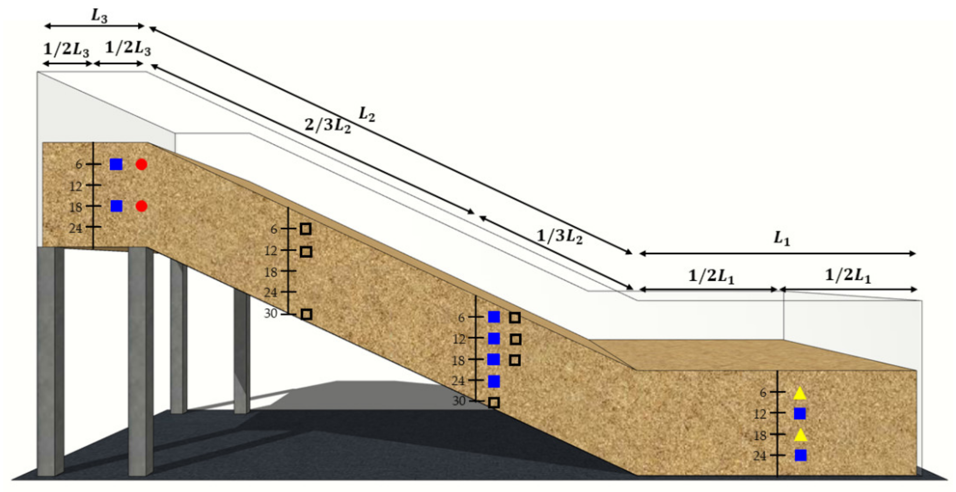


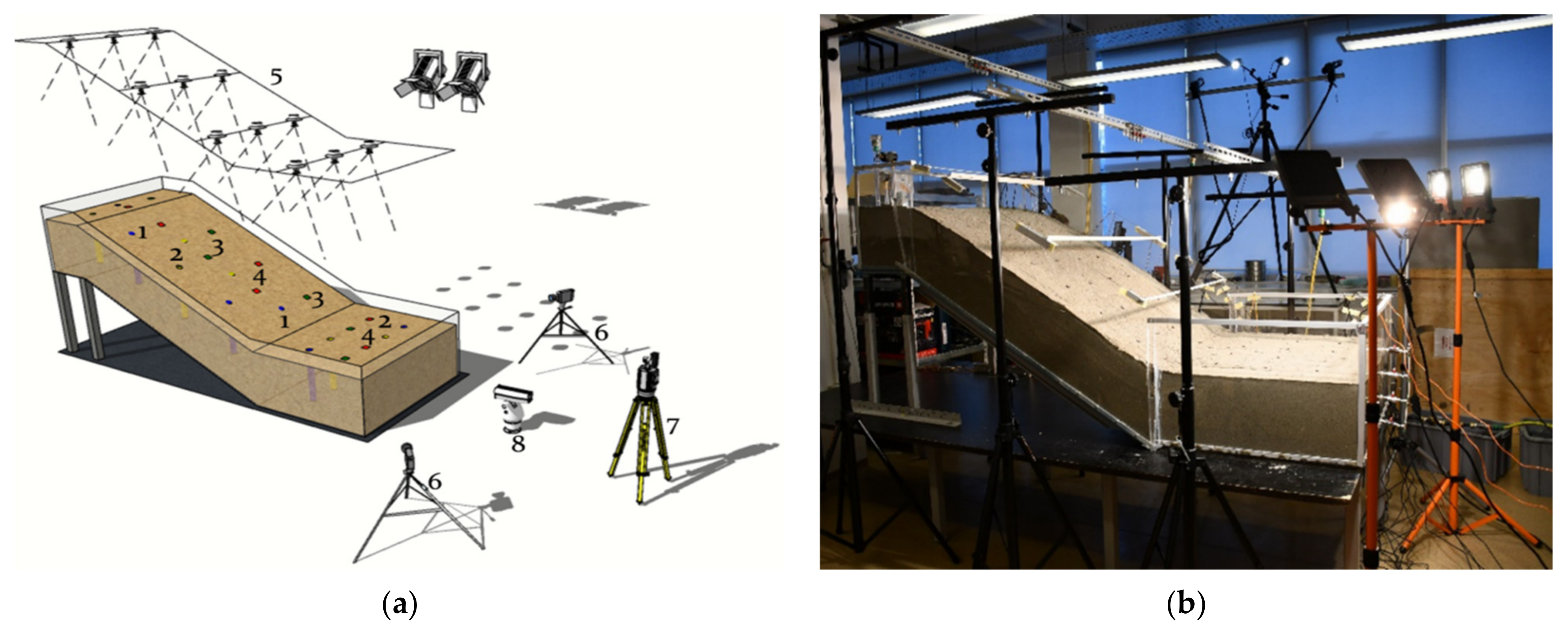
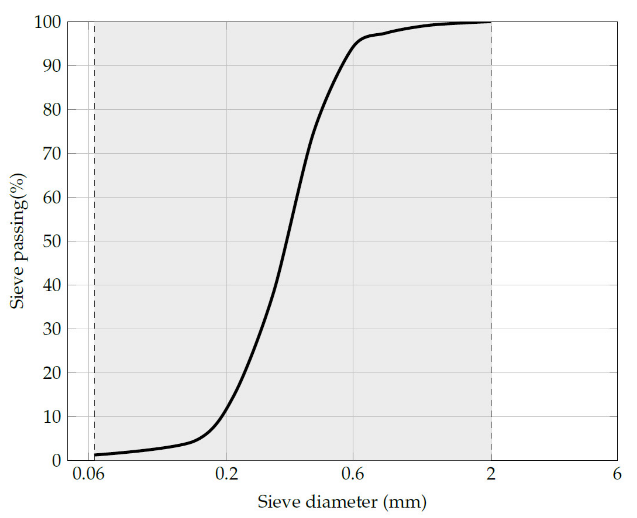
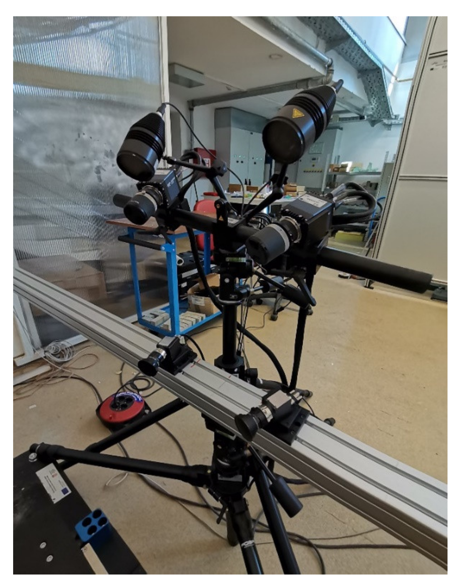
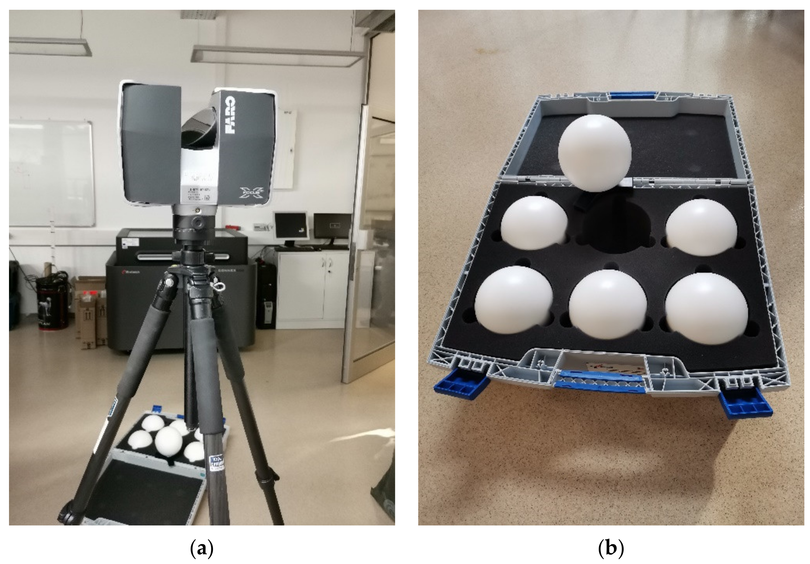
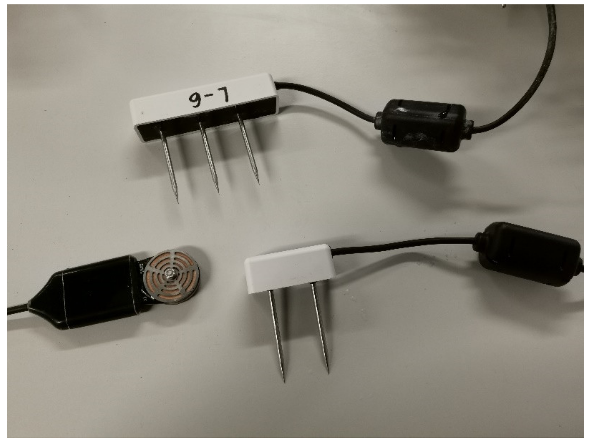
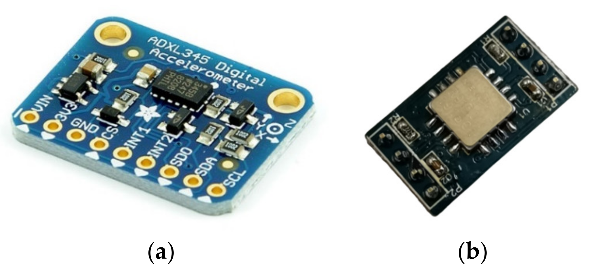
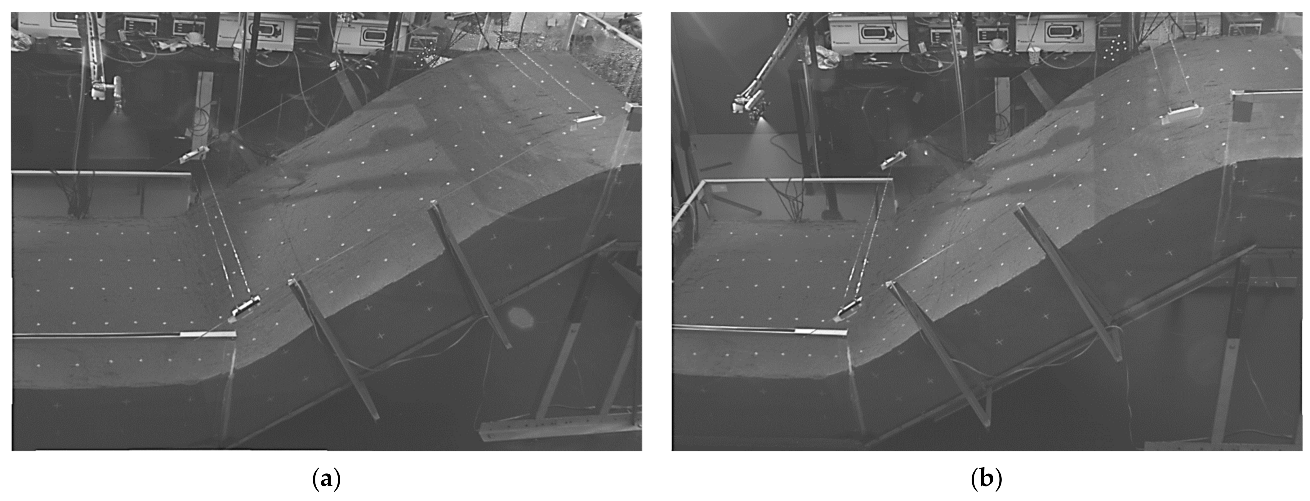
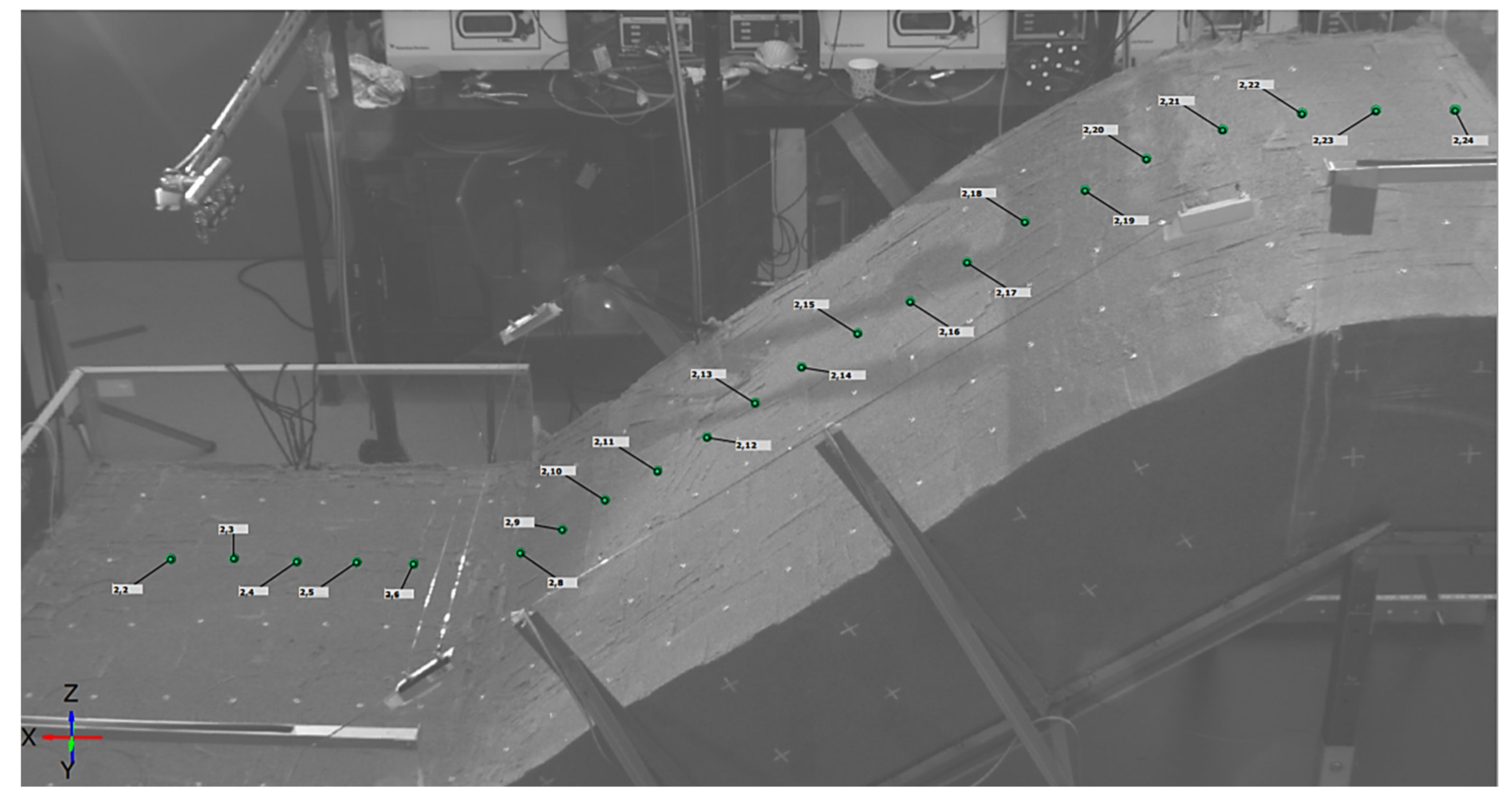
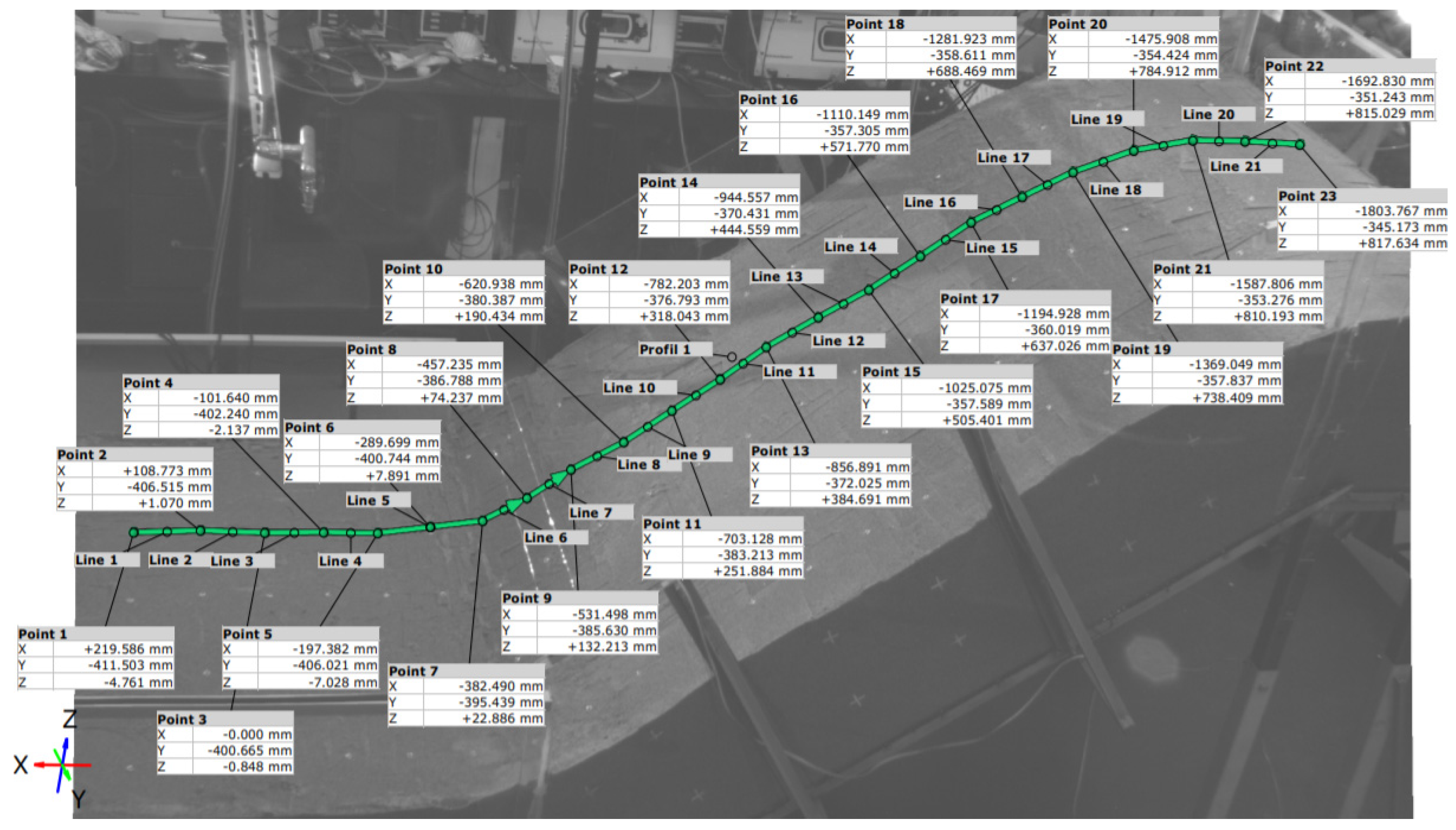
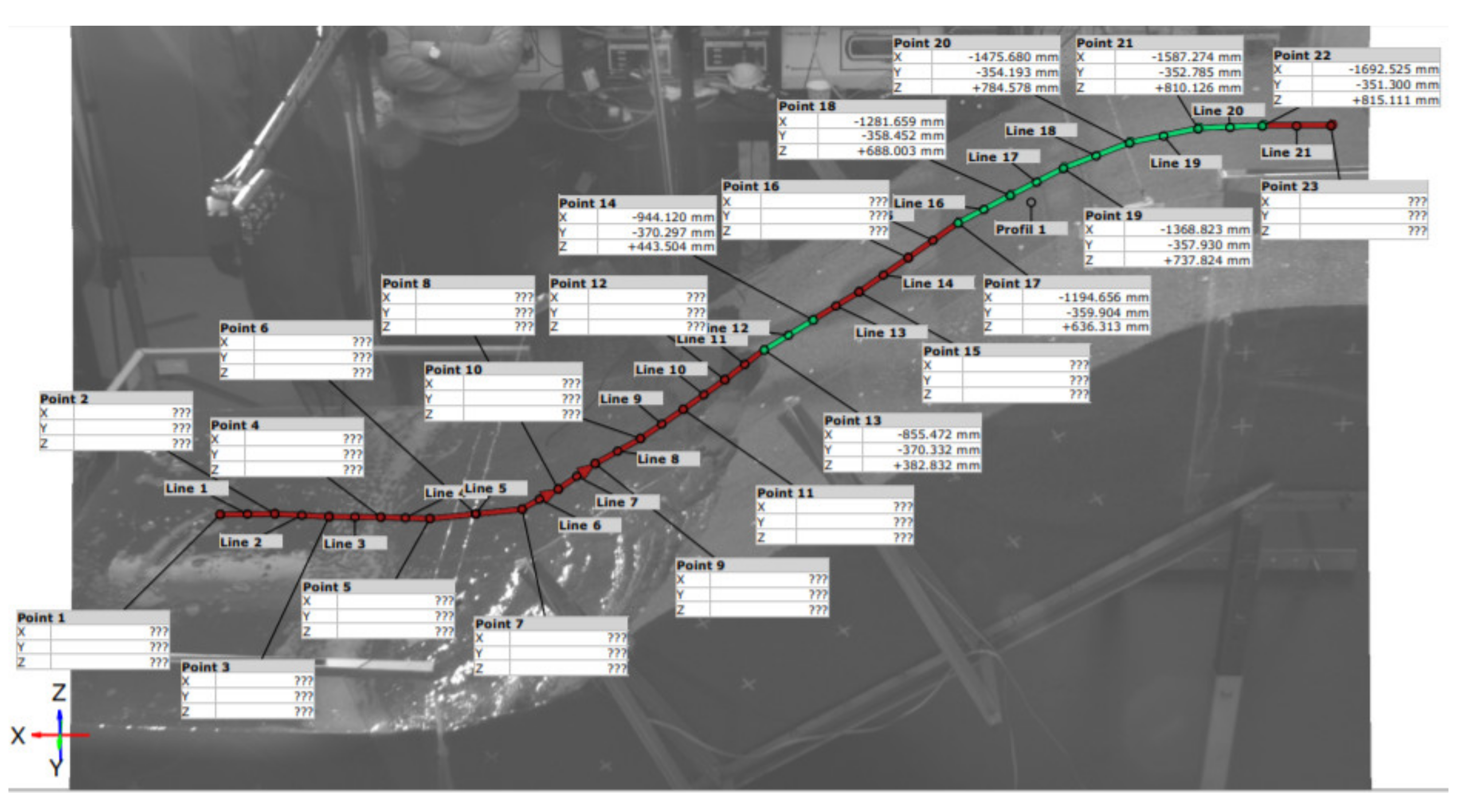
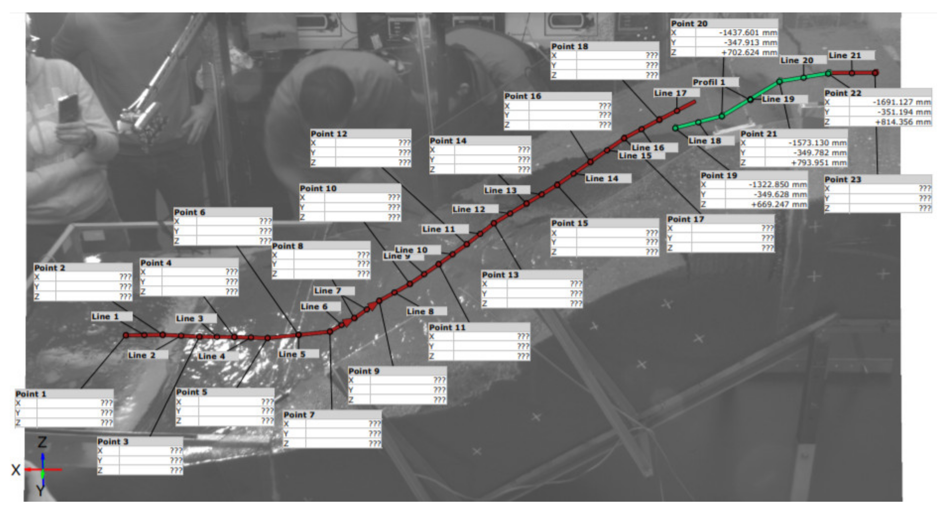
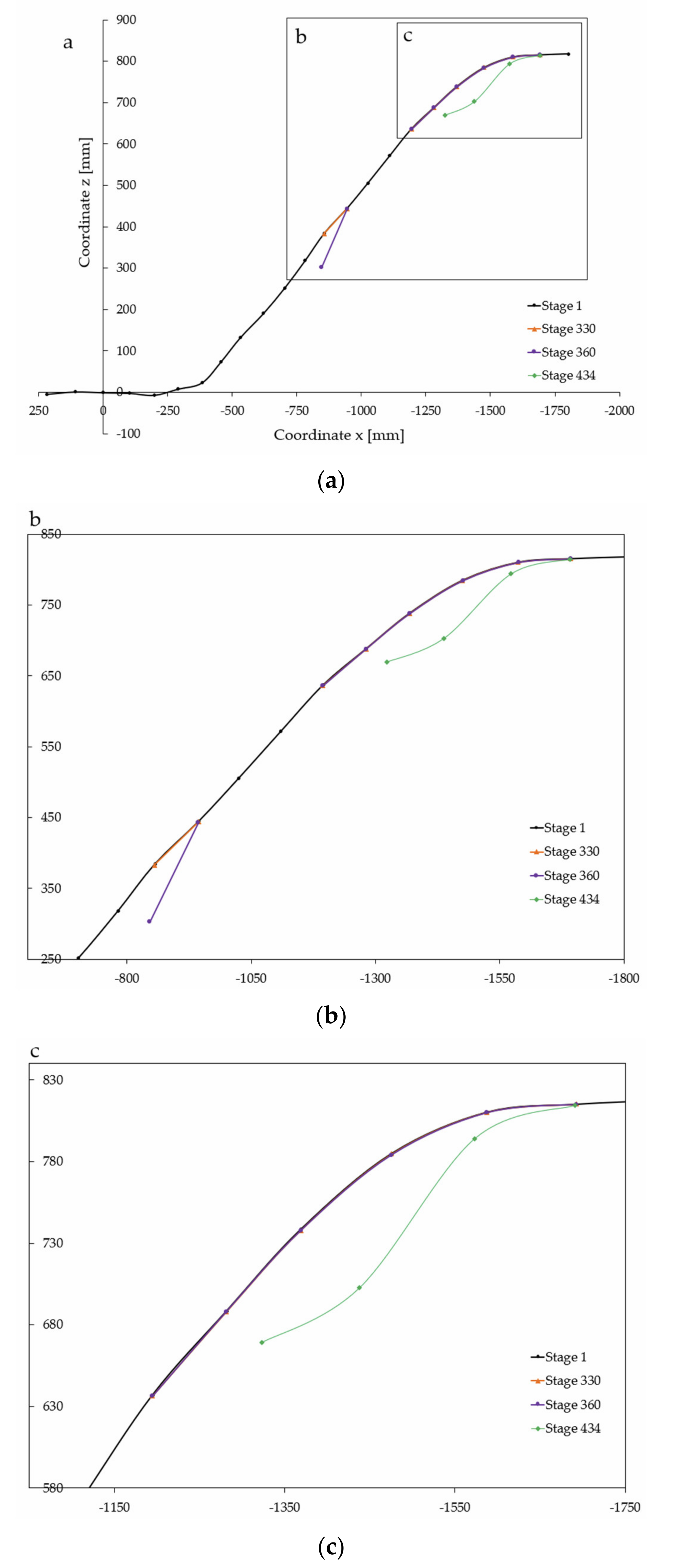
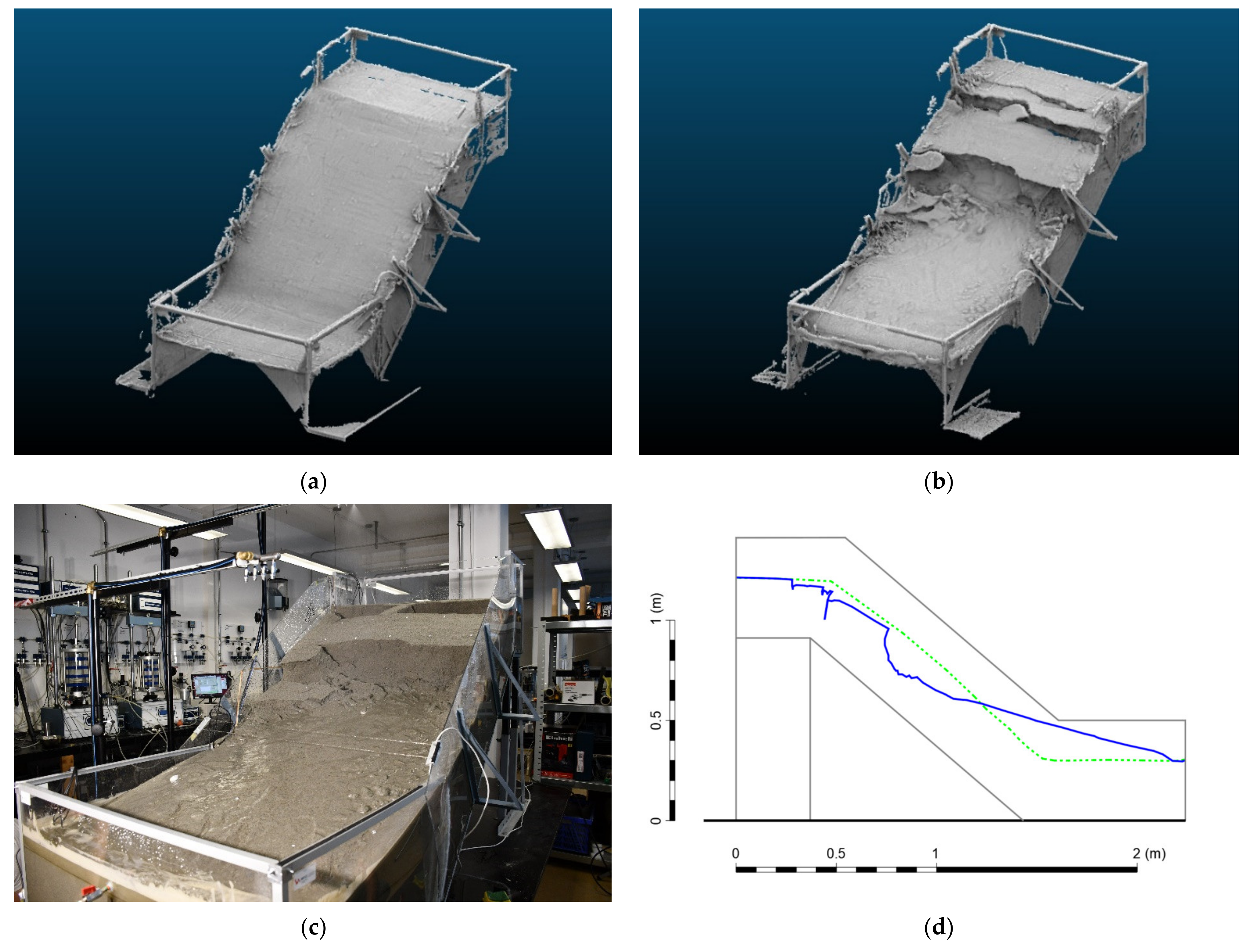
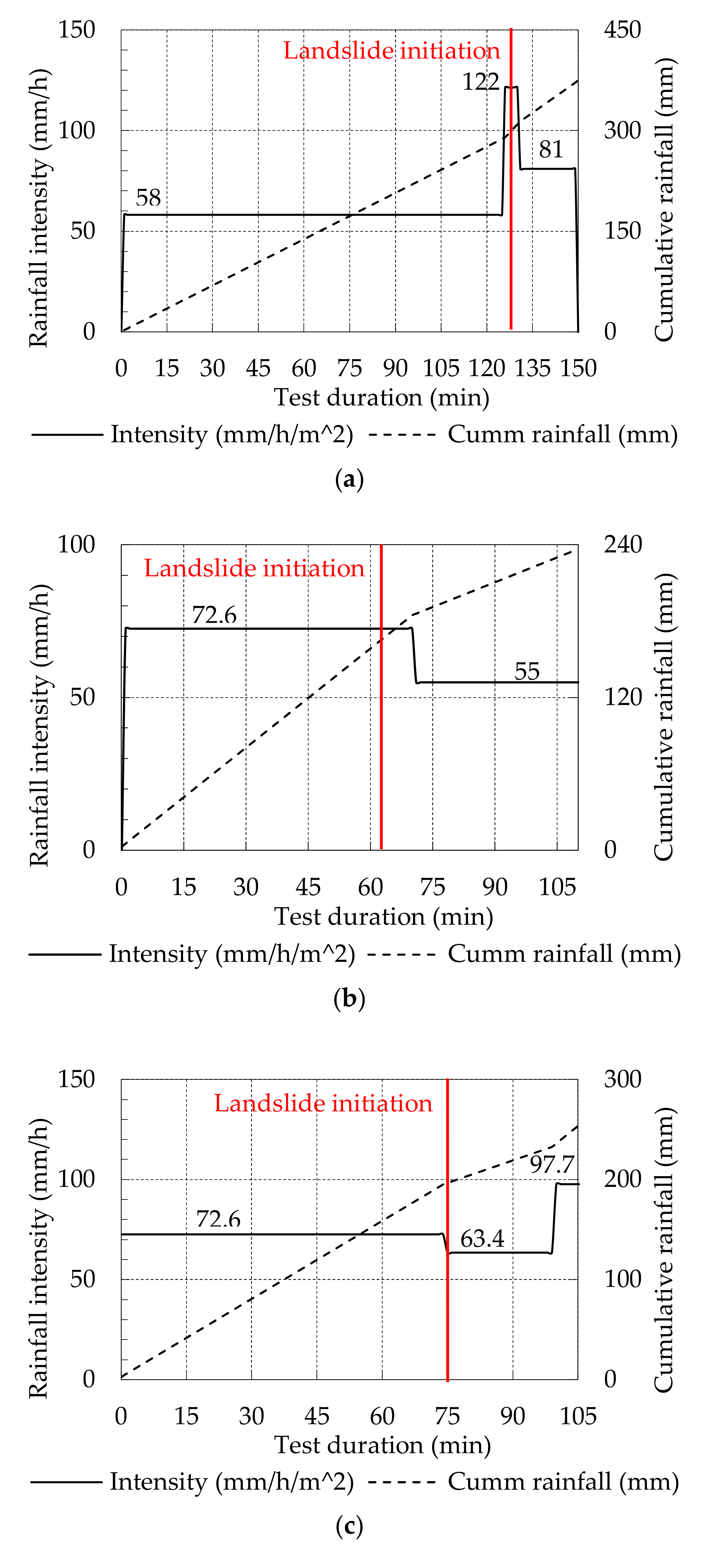
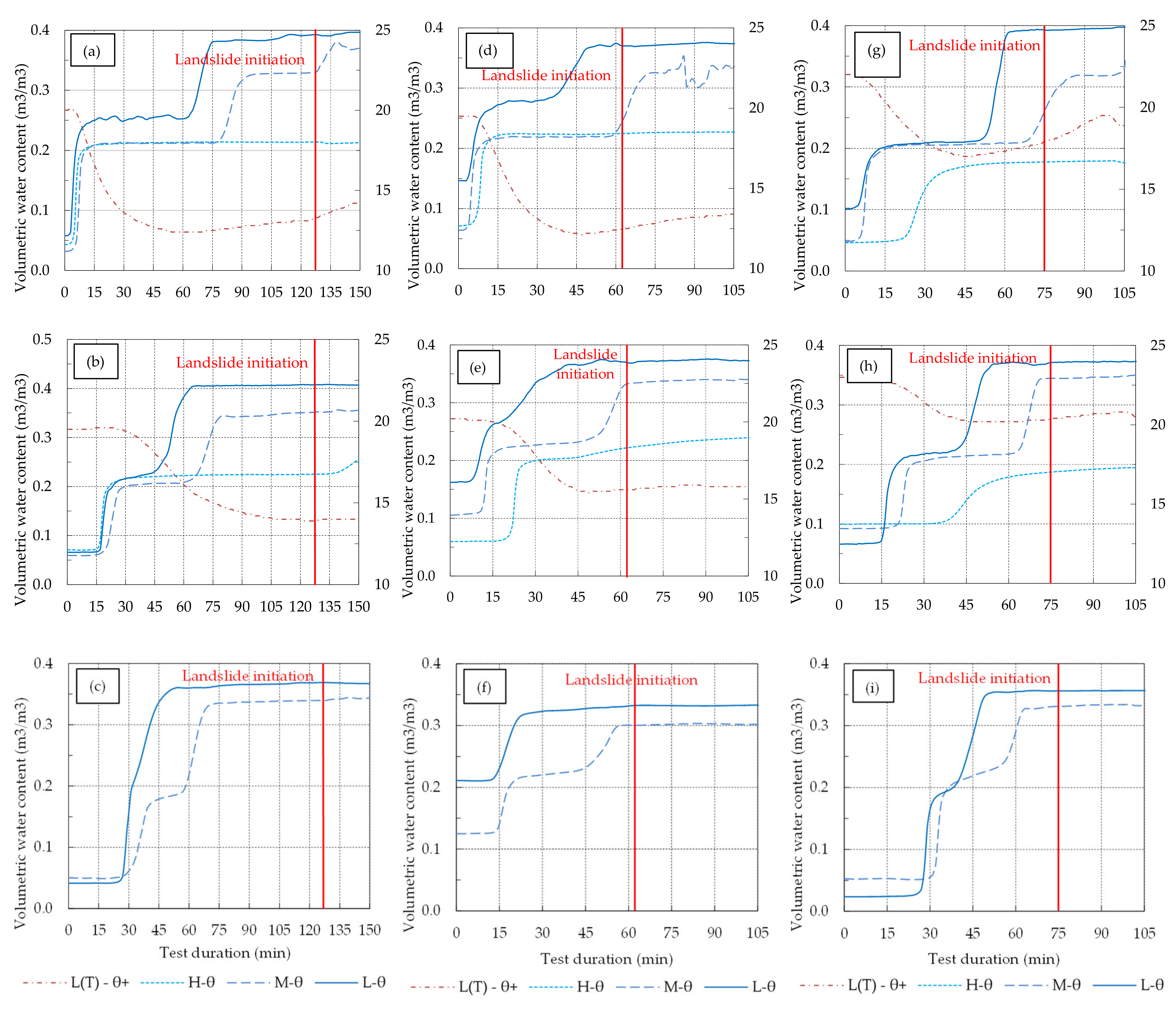