Deep Learning and Transfer Learning for Automatic Cell Counting in Microscope Images of Human Cancer Cell Lines

Abstract

In biology and medicine, cell counting is one of the most important elements of cytometry, with applications to research and clinical practice. For instance, the complete cell count could help to determine conditions for which cancer cells could grow or not. However, cell counting is a laborious and time-consuming process, and its automatization is highly demanded. Here, we propose use of a Convolutional Neural Network-based regressor, a regression model trained end-to-end, to provide the cell count. First, unlike most of the related work, we formulate the problem of cell counting as the regression task rather than the classification task. This allows not only to reduce the required annotation information (i.e., the number of cells instead of pixel-level annotations) but also to reduce the burden of segmenting potential cells and then classifying them. Second, we propose use of xResNet, a successful convolutional architecture with residual connection, together with transfer learning (using a pretrained model) to achieve human-level performance. We demonstrate the performance of our approach to real-life data of two cell lines, human osteosarcoma and human leukemia, collected at the University of Amsterdam (133 training images, and 32 test images). We show that the proposed method (deep learning and transfer learning) outperforms currently used machine learning methods. It achieves the test mean absolute error equal 12 (±15) against 32 (±33) obtained by the deep learning without transfer learning, and 41 (±37) of the best-performing machine learning pipeline (Random Forest Regression with the Histogram of Gradients features).

1. Introduction

Automatically analyzing microscope images is an important and challenging computer vision problem that can be done for a wide range of tasks. These include but are not limited to: classifying cell types [1,2], extracting cell shapes [3,4], identifying the position of cells [5,6,7], and counting the number of cells [8,9,10,11]. Counting cells in particular serves an important function for several different biomedical tasks. It has been used to aid in estimating microbial content [12,13], measuring cytotoxicity [14,15] and discovering the role of particular genes in cell biology, microbiology, and immunology [16,17,18]. For example, when conducting cancer research, researchers can investigate the effects of radiation using the clonogenic colony formation assay [19,20,21] or the neurosphere formation assay for measuring the proportion of brain tumor-initiating cells [22,23,24]. Manually counting cells is still conducted in some laboratories—frequently using hemocytometers as a visual aid [25]. However, this method is prone to interobserver variations, and it is arduous, time-consuming, and not feasible when using high throughput assays. Therefore, there is a need to count cells automatically.

In the last couple of decades, many computer-vision-based approaches have been suggested for automatic cell counting. The structure of these frameworks can be roughly categorized into two sections. First, hand-crafted feature representations are extracted that are further fed into a classifier. For instance, features are extracted using Histogram of Oriented Gradients (HOG) [26], Laplacian of Gaussian operation (LoG) [27], or Local Binary Patterns (LBP) [28] to represent the input images. Then the image representation is fed to a classification model such as a Support Vector Machine (SVM) or a Random Forest (RF) to detect the cells. However, approaches with hand-crafted features as input to classifiers could suffer from the following limitations: (i) Selecting a suitable feature extractor is a non-trivial task. Frequently, this requires specific knowledge of the cells in an image and the context wherein those cells are present. (ii) Feature extraction methods can be highly coupled with a specific type of cell, and, therefore, they do not generalize well to different images containing other cell types. (iii) Many feature extraction methods contain a large number of tunable parameters that highly affect the final performance. This makes the optimization process time-consuming and a matter of trial-and-error. (iv) Even with large datasets, the performance of such methods reaches a level upon which it cannot overcome anymore.

Deep Neural Networks (DNN) have been applied for a wide range of computer vision tasks and has set new state-of-the-art on several benchmarks related to classification, object detection, and segmentation [29,30,31,32,33]. The biggest advantage of using deep neural networks is that there is no need to rely on hand-crafted features anymore. Instead, a deep neural network is optimized using a (mini-batch) gradient descent over large amounts of data and automatically learns problem-specific features directly from training data. With regards to the problem of counting cells in images, this task can be approached from two distinct directions: (i) developing a cell detector, and (ii) developing a cell counter.

Cell detection approaches consider the problem as a matter of identifying cell instances in an image first and then counting the number of instances found. Frequently, these approaches rely on each image containing annotation information, consisting of either dot annotation localizing the centroids of cells [34,35,36], or bounding box annotations indicating the borders of cells [37]. The problem with these approaches is that using them in real-world applications is challenging because cell densities can be extremely high, ranging in the thousands per image, and cells can have wide varieties regarding shapes, sizes, and colors. A different approach relies on applying semantic segmentation and predicting the spatial density [38] or density maps [39]. However, these methods require pixel-level annotations of the images during training, which is typically hard to acquire due to high costs.

Counting by regression, on the other hand, directly predicts the number of target instances in an image rather than detects the number of objects present. Various machine learning and deep-learning approaches are available for a regression task, such as Support Vector Regression (SVR) [40], Random Forest Regression (RF) [41], Nearest-neighbor regression (NNR) [42], and Ridge Regression (RR) [43]. Counting by segmentation can be considered to be a mix of the counting by detection and counting by regression method since cells are first segmented before they are regressed. For example, in [44] a Feature Pyramid Network was used to segment the images by first building a ground truth feature mask, before regressing on that feature mask. Although this method is less labor-intensive than methods that require annotating, it cannot overcome limitations such as cell clumping and overlap.

More generally, all methods that require obtaining annotations for the entire training data are time-consuming and expensive, especially if we are only interested in the global count of cells, and not in additional information such as their shapes, sizes, or locations. When it comes to developing a cell counter, the problem could be considered to be a regression task, whereby we are interested in learning the relationship between image representations (which are usually image global features) and the number of cells present [45,46]. The problem is, however, that many of these approaches treat the regression problem as a multi-class classification task. This means that the number of cells is considered to be a class ID, and images with the same number of cells belong to the same class. As a result, a model will view images with 2 cells or 500 cells just as far apart as images containing 50 and 51 cells. In other words, they are unable to properly learn ordering. Thus, it is important to model this task as a regression problem rather than a multi-class classification problem.

Here, we propose use of a Convolutional Neural Network (CNN) that directly predicts the number of cells, i.e., it is a regression model. As a result, our approach does not require pixel annotations, which are typically very costly to obtain, which drastically improves its wide applicability. We will demonstrate that in comparison to approaches with hand-crafted features as input to a regressor, our method not only provides better performance, but it is also easy-to-use. Moreover, we present that the application of the transfer learning is essential to achieve a high performance when a small number of data are available.

The contribution of this paper is three-fold:

• A novel dataset containing images and the number of manually counted cells is presented. The images represent a human osteosarcoma cell line (U2OS) and a human leukemia cell line (HL-60). The dataset was collected at the University of Amsterdam, and could be downloaded from: https://doi.org/10.5281/zenodo.4428844 (accessed on 26 May 2021).
• The development of a pipeline for automatically counting cells using a convolutional neural network-based regressor. We indicate a specific architecture of a neural network that in combination with transfer learning allows the achievement of very promising performance.
• We provide baseline results for the newly collected data. Moreover, we present that the proposed approach achieves a human-level performance.

2. Methodology

2.1. Problem Statement

We consider the problem of counting cells as a regression task. Let $x\in {\mathbb{R}}^{C\times H\times W}$ denote an image with C channels (e.g., RGB), height H and width W. Furthermore, let $y\in \mathbb{R}$ be several cells present in x. The regression model F transforms the extracted features from x, $\varphi \left(x\right)$, to the number of cells, i.e.:

$$y=F\left(\varphi (x;a);\theta \right),$$

(1)

where $a\in {\mathbb{R}}^D$ denotes the parameters of a feature extractor, and $\theta$ stands for parameters of the regression model F.

For given N datapoints, $\mathcal{D}={\left\{(x_n,y_n)\right\}}_{n=1}^N$, we aim to minimize a given loss function $\mathcal{L}$ with respect to a and $\theta$, i.e.:

$$\mathcal{L}(a,\theta ;\mathcal{D})=\frac{1}{N}\sum _{n=1}^N\ell (a,\theta ;x_i,y_i),$$

(2)

where, typically, $\ell (a,\theta ;x_i,y_i)={\left(y_i-F(\varphi (x_i;a);\theta )\right)}^2$, and $\mathcal{L}$ is then known as the Mean Squared Error (MSE) loss.

We consider two approaches for automatic cell counting, namely a machine learning pipeline and a CNN-based regressor. In the following sections, we explain the components of these two approaches. For the machine learning pipeline, we outline different feature extractors and nonlinear regressors. Next, we present our proposition of the CNN-based regressor with a specific architecture of the CNN, namely xResNet [47,48].

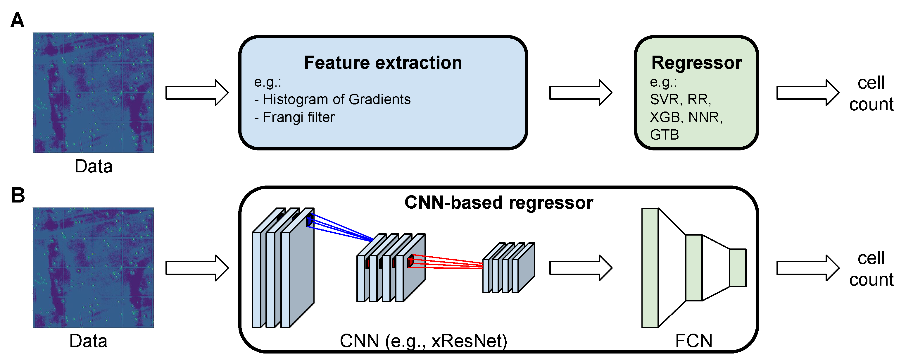
2.2. Machine Learning Pipeline

A crucial component for a successful regressor is the feature extraction. There are many feature extraction methods available for image processing [49]. Here we focus on two feature extractors: Histogram of Oriented Gradients (HOG) and Frangi filter. Next, once features are extracted, the regression model is used to predict cell counts. The simplest approach would be to apply linear regression. However, nonlinear models, e.g., Support Vector Regression, XGBoost are preferred due to their flexibility. As a result, we obtain a two-stage pipeline (see Figure 1A) that consists of: (i) a feature extraction method, (ii) a regression method. Each stage is optimized separately. We refer to this approach as the machine learning pipeline.

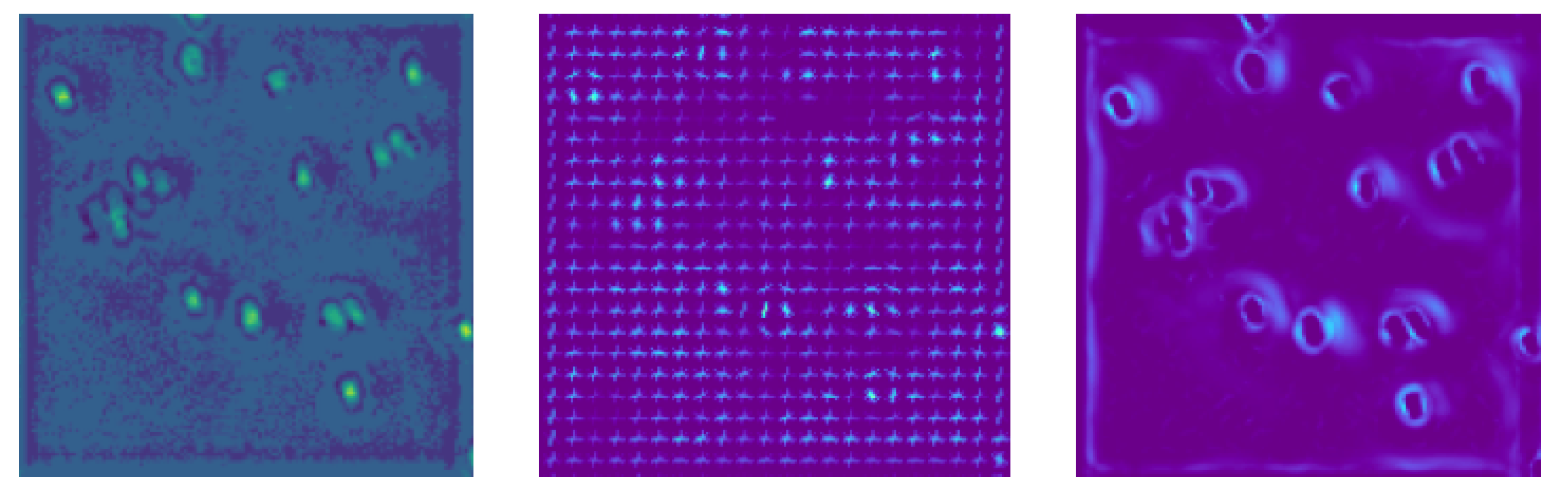
2.2.1. Feature Extractors

In this paper, we consider two feature extractors, namely Histogram of Oriented Gradients (HOG) and the Frangi Filter. HOG is considered one of the best-performing feature extractors in computer vision, while the Frangi Filter is widely used in medical imaging.

HOG

A Histogram of Oriented Gradients [26] is a commonly used feature descriptor for extracting features from image data. It works by extracting the distribution of orientations of gradients of an image. Intuitively, these gradients are useful because the magnitude is large around edges and corners, since these regions contain abrupt intensity changes, and could be indicative of a cell being present. An example of the output of the HOG feature extractor is presented in Figure 2 (Middle).

Frangi Filter

The Frangi filter was applied to medical images [50]. Although this was originally designed and still applied to detect vessel-like or tube-like structures and fibers [51,52], some preliminary exploratory research demonstrated that this filter was also effective for our task. An example of the output of the HOG feature extractor is presented in Figure 2 (Right).

2.2.2. Regressors

In machine learning, there are multiple possible regression models. Here, we present five widely used regressors that are applied to extracted features, namely: Support Vector Regression [53], XGBoost [54], Ridge Regression [55], Nearest-Neighbor Regression [42], Gradient Tree Boost [56].

Support Vector Regression

One of the most popular machine learning tool for classification is the Support Vector Machines (SVM), first introduced in [57]. Many variations have been introduced since then, and we will focus on the Epsilon Support Vector Regression, whereby the goal is to find a function F that does not deviate more than $ϵ$ from $y_n$ for each training point $x_n$, and is as flat as possible. The resulting regressor takes the following form:

$$F(\varphi \left(x\right);\theta )=\sum _{n=1}^N({\theta }_n-{\widehat{\theta }}_n)k(\varphi \left(x_n\right),\varphi \left(x\right))+{\theta }_0,$$

(3)

where $k(\varphi \left(x_n\right),\varphi \left(x\right))$ is a kernel function, and ${\theta }_n$ and ${\widehat{\theta }}_n$ follow from the solution of the dual formulation [57].

Gradient Tree Boosting

Gradient boosting is a common machine learning method where multiple weak prediction models (usually CART tree learners) are combined into one predictive model.

The regression gradient boosting algorithm was first introduced in [56] and it modifies this algorithm such that it chooses a separate optimal value ${\gamma }_{jm}$ for each of the tree’s regions $R_{jm}$, instead of a single ${\gamma }_m$ for the whole tree. Then, the update rule for the model becomes:

$$F_m\left(x\right)=F_{m-1}\left(x\right)+\sum _{j=1}^{J_m}{\gamma }_{jm}{\mathbf{1}}_{R_{jm}}\left(x\right),$$

(4)

$${\gamma }_{jm}=\underset{\gamma }{arg\; min}\sum _{x_i\in R_{jm}}L(y_i,F_{m-1}\left(x_i\right)+\gamma ).$$

(5)

XGBoost

XGBoost is an improved version of previously developed gradient boosted models (GBM) [54]. However, GBM builds trees sequentially, XGBoost is parallelized, therefore making the algorithm much faster. In addition, XGBoost also includes regularization in the objective function, which punishes more complex models and prevents overfitting.

Ridge Regression

The ridge regression is a popular variation to linear regression that adds L2 regularization to the loss function, hereby preventing overfitting to the training data. Let $\lambda >0$ be a regularization factor. Then the penalized loss function in the ridge regression can be formulated as follows:

$$\mathcal{L}(\theta ;\mathcal{D})=\frac{1}{N}\sum _{n=1}^N{(y_n-\sum _{j=1}^p{x}_{nj}{\theta }_j)}^2+\lambda \sum _{j=1}^p{\theta }_j^2.$$

(6)

Nearest-Neighbor Regression

The Nearest-Neighbor algorithm is a non-parametric regression introduced in [58]. It works by predicting target values through interpolation of the targets of k nearest neighbors in the training set, scaled by a weighting factor. Most commonly they are weighted by the inverse of their distance.

2.2.3. Remarks

The machine learning pipeline works fairly well in practice; however, there are still some issues with it. First, the range of possible methods for extracting features is broad, and the same could be said about choosing a regressor. In [59] alone, they mention 35 different feature extractors, while a plethora of regression techniques have been described in the literature. Second, even with a perfect understanding of a feature extractor or a regressor’s inner workings, it is not possible to predict exactly how well it will perform on a dataset for a given task. In general, it is very difficult to predict which combination of a feature extraction method and a regressor will perform well. Taking into account these issues, neural networks seem to constitute a more suitable class of models due to their flexibility and adaptivity to a broad class of problems, including our task of cell counting.

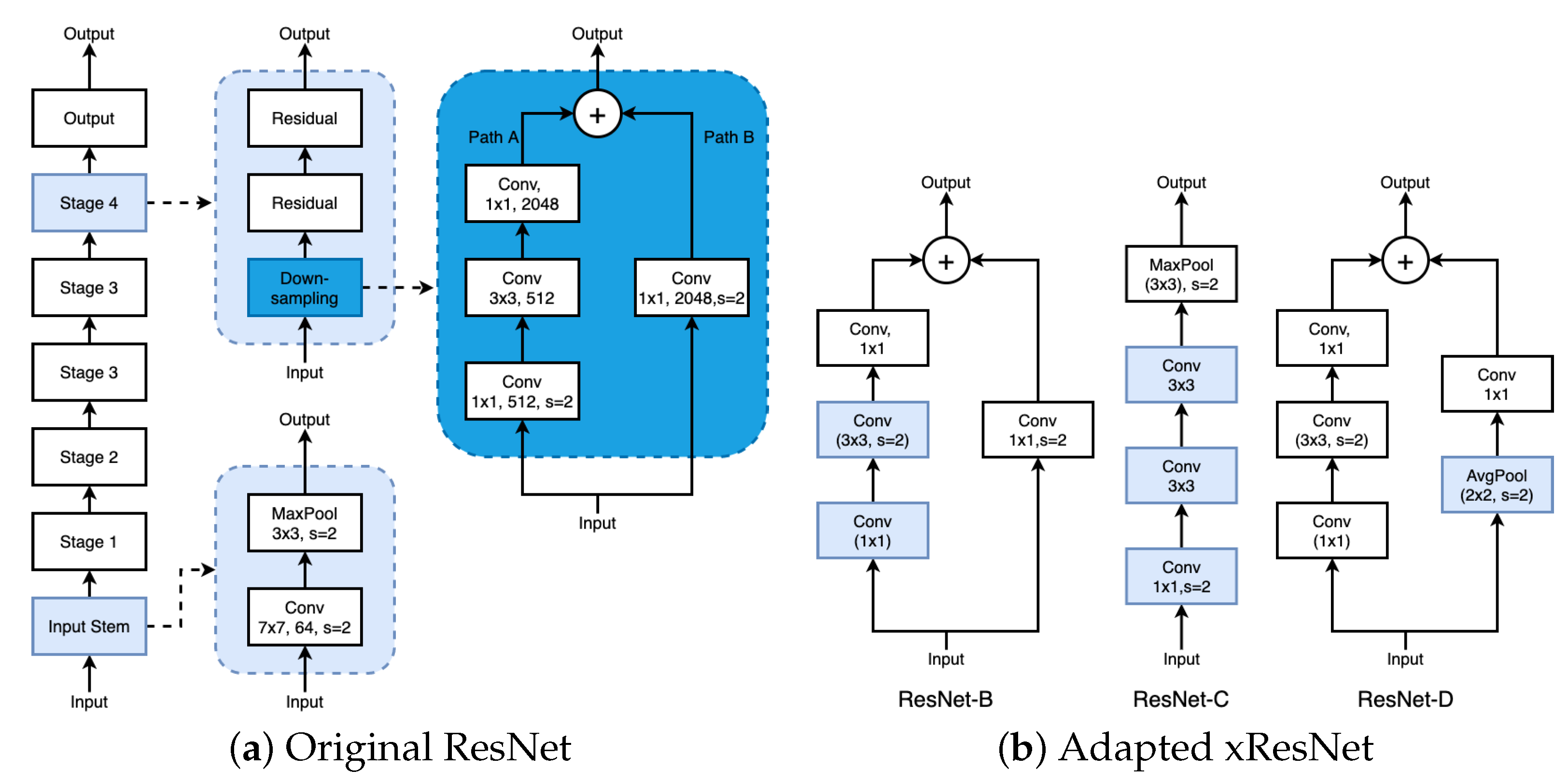
2.3. CNN-Based Regressors

Alternatively, we can consider a deep-learning-based approach. Instead of selecting various methods and optimize them separately, we could train a single model end-to-end, in which a feature extractor and a regressor are modeled by deep-learning building blocks (e.g., convolutional and fully connected layers, residual blocks). Such an approach has been proved to be successful for counting cells but in the classification task, see [60]. Here, we propose combination of a convolutional neural network (CNN) with a regressor (a fully connected neural network, FCN) to predict the cell count directly (see Figure 1B), without segmenting cells and then counting them. We refer to this approach as a CNN-based regressor.

2.3.1. Neural Network Regression

The main advantage of neural networks is that instead of selecting a pair of a feature extractor and a regression model, we select an architecture that allows learning features and predicting cell counts. Moreover, the learning process is end-to-end that significantly simplifies the optimization, and increases adaptive capabilities to a specific problem or data. Moreover, a neural network regression relies only on pixel intensities, whereas other cell counting approaches commonly require additional information, such as the cell’s shape, size, and location.

As mentioned previously, manually extracting features is time and labor-intensive and its performance is hard to predict. Therefore, deep-learning-based models and especially Convolutional Neural Networks (CNN) have become more popular among researchers and practitioners. Because their architecture is intrinsically hierarchical, CNNs can automatically and adaptively learn multi-level hierarchies of features that are translation-equivariant [61]. This means that inside of the CNN, early layers will learn low-level features such as edges, textures, and boundaries, while deeper layers can learn high-level semantic features that are close to the target labels.

The CNN architecture usually consists of several building blocks, such as convolutional layers, pooling layers, and fully connected layers, whereby the first two layers are repeated multiple times, followed by one or more fully connected layers. In the convolutional layers, features are extracted through a combination of linear and nonlinear operations, i.e., a convolutional operation whereby a kernel is applied across the input and nonlinear activation functions such as the rectified linear unit (ReLU) and its variants. In the pooling layers, feature maps are typically downsampled to introduce translation invariance to small shifts and distortions and to decrease the number of learnable parameters. Max pooling and global average pooling are most commonly used. The output feature map of the last convolutional layer is commonly flattened and connected to one or more fully connected layers.

As for obtaining large amounts of high quality, labeled data in medical imaging is seldom available because of the cost and necessary workload of radiology experts, transfer learning is often applied. With transfer learning, a network is pretrained on an extremely large dataset, such as ImageNet, and then applied to a different task in a different domain [62]. The underlying notion is that early layers in this network are already trained to recognize low-level features and that these features can be shared across unrelated datasets. This makes transfer learning particularly useful for small datasets.

2.3.2. Our CNN-Based Regressor

In this paper, we propose use of the deep residual network architecture (ResNet) as introduced in [63]. In contrast to other CNN architectures, the ResNet consists of several residual blocks, which are composed of a convolutional layer, a batch normalization layer, and a shortcut that connects the original input to the output of the residual block. Figure 3a shows schematically how a Residual Block with Identity Shortcut (RB-IS) and a Residual Block with Projection Shortcut (RB-PS) operate. Mathematically, the residual block can be summarized as follows:

$$h_l=F(h_{l-1},\left\{W_l\right\})+G\left(h_{l-1}\right),$$

(7)

where and $h_{l-1}$ is the output of the $l-1$-th layer, F is the residual function (e.g., a composition of convolutional layers, batch-norm layers, pooling-layers, and nonlinear activations such as ReLU), G corresponds to the shortcut connection, and $G\left(h_{l-1}\right)$ could be either the identity map, $G\left(h_{l-1}\right)=h_{l-1}$, or a projection, $G\left(h_{l-1}\right)=W_p{h}_{l-1}$, $W_l$ denote weights of a residual block, and $W_p$ stands for weights of the projection. If the dimensions of $h_{l-1}$ and $h_l$ are the same, the identity shortcuts are used; otherwise, a projection mapping is applied, meaning a linear projection $W_p$ is performed on the shortcut connections to match the dimensions.

The main idea of the ResNet is to learn the additive residual function F with respect to $G\left(h_{l-1}\right)$, with the choice to use an identity mapping and/or projection mapping. In our implementation, we changed the last fully connected layer of ResNet to output 1 scalar instead of the original 1000-D vector. In addition, the SoftMax loss function was replaced with MAE loss.

In this paper, we used xResNet, which is a modified version of the original ResNet architecture, which has shown to increase accuracy, and provide improved performance for transfer learning tasks, compared to ResNet architectures [47]. xResNet applies a couple of small tweaks compared to the original architecture. The first one is shown in Figure 3b as ResNet-B in which the A path is altered in the downsampling block by moving the stride of 2 to the second convolution and keeping a stride of 1 for the first layer.

The second modification can be seen in ResNet-C (Figure 3b): the 7 × 7 convolution is removed in the input stem of the network and replaced with three consecutive 3 × 3 convolutions, whereby the first one has a stride of 2 and the other two a stride of 1. The third modification is present in ResNet-D (Figure 3b): the path B of the downsampling layer is modified by adding average pooling with a stride of 2, before a convolution with a stride of 1, and not 2.

For our purposes, we propose use of xResNet50, which consists of an input stem, four stages with each varying amounts of xResNet blocks, and an output stem. In the input stem there are three convolutional layers, each followed by batch normalization, and a ReLU. In between the input stem and the first of the four stages there is a max pooling layer. The first stage consists of three xResNet blocks, the second stage of four xResNet blocks, the third stage of six xResNet blocks, and the fourth stage of three xResNet blocks again. In between the fourth stage and the output stem, there is an average pooling layer. In the output stem the input is first flatted and dropout is applied, before the final fully connected linear layer, which has 1 output. In total there are trainable 23,529,313 parameters.

3. Experiments

3.1. Dataset

• Data Information

For cell counting, two cell lines were used, namely a human osteosarcoma cell line (U2OS) and a human leukemia cell line (HL-60). Osteosarcoma is a primary malignant form of bone cancer. Generally, it affects children and adolescents, where it represents the eighth-most common form of childhood cancer. Considering its poor prognosis, it is the second most important cause of deaths related to cancer in both children and adolescents [64,65]. Cells from the U2OS cell line originate from bone tissue, from a differentiated sarcoma of the tibia. Moreover, U2OS cells are epithelial adherent cells and exhibit a fast growth rate. HL-60 is a cell line that was originally derived from a woman suffering from acute promyelocytic leukemia. This type of blood cancer is a subtype of acute myeloid leukemia. Untreated, the median survival is less than one month [66].

The U2OS and HL60 cell lines were cultured in Roswell Park Memorial Institute 1640 medium (RPMI; GibcoBRL, Grand Island, NY, USA) and Dulbecco’s Modified Eagle Medium (DMEM; GibcoBRL, Grand Island, NY, USA), respectively, supplemented with $10\%$ Fetal Bovine Serum (FBS) and $1\%$ antibiotics (penicillin and streptomycin). To determine the number of cells growing in medium, hemocytometer counting was performed according to the ABCAM protocol ‘Counting Cells Using a Hemocytometer’ with minor modifications. Visualization and counting of the cells was done using microscope Axiovert S100 from Zeiss, with a 10X objective. The mean number of cells was determined by repeatedly counting cells in four non-overlapping sets of 16 corner squares, indicated on the hemocytometer, selected at random. A camera and computer program from Zeiss, AxioCam Cm1 and ZEN 2 respectively, were used to capture and save snapshots of the hemocytometer containing the cells. These microscope images could then be used for experiments.

• Data Preparation

The images were originally in the Carl Zeiss Images (.czi) format, a microscope image file format commonly containing image stacks, time-lapse series, and tile images captured from a Carl Zeiss microscope. In contrast with regular image formats, czi can combine imaging data with additional metadata about the image itself, the microscope, and the camera used. The files in this dataset, however, only contained metadata on the images, i.e., its size (1388 by 1038 pixels with 1 channel), and its pixel type (‘gray16’). In the filename, the number of cells present in the inner 16 squared grid was given. Using the aicspylibczi library (https://pypi.org/project/aicspylibczi/ (accessed on 26 May 2021)) the images were loaded as Numpy arrays and saved in the TIFF format using the Pillow Image module (https://pillow.readthedocs.io/ (accessed on 26 May 2021)). Next, the grid of 16 inner squares was manually cropped because only cells in this area were counted and represented in its label. This resulted in images of 700 by 700 pixels. The OpenCV library was used to handle images in the tiff format.

When looking at the original images in Figure 4, it can be observed that the following challenges are present:

• The cells tend to have varying circularity ratios, ranging from elongated ellipses to round circles. Therefore, algorithms that rely on the round shape assumption do not hold.
• Some cells have differing levels of staining intensity. Therefore, algorithms that require homogeneous intensity distributions of the object will not perform well.
• Since cells were manually counted using counting chambers, the grid lines are still present in the image. These will cause interference with algorithms that separate foreground from background.

Altogether, we have obtained 165 images that we randomly split into the training set (133 images) and the test set (32). To compare all methods in a fair manner, we kept this training-test split fixed. Moreover, we decided to keep this split fixed for future comparisons and reproducibility. The data are available online at: https://doi.org/10.5281/zenodo.4428844 (accessed on 26 May 2021).

• Data Augmentation

Since we have a low number of images compared to image size (700 × 700 pixels), we used data augmentation [67,68]. We used transformations that manipulate the orientation, brightness, and contrast of the cropped cell images. Each cell was randomly mirror-flipped along the vertical and horizontal axes, and the brightness and contrast were randomly adjusted (by a 20% strength with a probability of 75% of occurring). In our preliminary experiments, training without data augmentation resulted in overfitted models, which is a known fact in the computer vision field [68].

3.2. Details of the Machine Learning Pipeline

In this work, we implemented and verified five different machine learning techniques, namely: Support Vector Regressor (SVR), Ridge Regression (RR), Nearest-Neighbor Regression (NNR), XGboost, and Gradient Tree Boosting (GTB). For each of these approaches, in the preliminary experiments, we analyzed the following feature extractors: Multi-dimensional Gaussian filtering, Frangi filtering, Hybrid Hessian filtering, Laplace operator filtering, local median filtering, Meijering filtering, Roberts’ filtering, ISODATA threshold-based filtering, Li’s filtering, local mean threshold-based filtering, Niblack, Otsu, Sauvola, Yen’s filtering. Since the Frangi filtering gave the best preliminary results, further experiments were conducted using that method only. Additionally, we used the Histogram of Oriented gradients since it is one of the state-of-the-art feature extractors in computer vision.

The machine learning pipeline was implemented using Scikit-Learn (https://scikit-learn.org/ (accessed on 26 May 2021)). The SVR was trained with kernel type ’Radial Base Function’ with 3 degrees, and the stopping criterion at $0.001$. The Ridge Regression was trained using alpha = 1, and tol = 0.001. The Nearest-Neighbor regressor was trained with 3 neighbors, uniform weights, leaf size = 30. XGboost (we used the implementation available at: https://xgboost.readthedocs.io/ (accessed on 26 May 2021)) was trained with learning rate = 0.1, max_depth = 5, alpha = 10. The Gradient Tree Booster was trained using learning rate = 0.1, and max_depth = 1.

3.3. Details of Our Approach

A pretrained model was used to initialize the xResNet (we used the network xResNet50 available at: https://docs.fast.ai/vision.models.xresnet.html (accessed on 26 May 2021), which is pretrained on ImageNet data). The entire network was trained for 400 epochs, where an epoch represents one training pass through all training instances. Training employed a momentum-based gradient optimization with momentum linearly increasing from 0.85 to 0.95 in the first 30% of epochs (133 epochs), and for the remaining 70% (267 epochs) the momentum decreased from 0.95 to 0.85. Furthermore, learning rates were scheduled using cosine annealing with a base learning rate at 0.002 [69]. No weight decay was applied to bias and batch normalization layers. For the first epoch, all but the last layer was frozen, meaning that only the weights of the last layer were updated with a fixed learning rate of 0.002. Then for 399 epochs, the entire network was unfrozen and trained using learning rate scheduling with cosine annealing and the one-cycle training policy as introduced by Smith [70].

The proposed CNN-based regressor was implemented in Python using PyTorch and Fastai package [48]. All the experiments are run on a machine with Intel Xeon CPU @ 2.2 GHz × 2 and GPU Nvidia Tesla V100-SXM2-16GB.

3.4. Evaluation Metric

In all the experiments we used the Mean Absolute Error (MAE) as the metric to quantitatively evaluate the performance that is defined as follows:

$$MAE=\frac{1}{N}\sum _{i=1}^N|t_i-y_i|,$$

(8)

where N is the total number of images, $t_i$ and $y_i$ are the true and predicted numbers of cells in the i-th test image, respectively. We prefer MAE over MSE because MAE could be easily interpreted (the same unit as the original cell count, while MSE provides the squared error).

4. Results and Discussion

We present the results for machine learning-based regressors in Figure 5 and for our proposed CNN-based regressor in Figure 6 and Figure 7. We gather all results (average ± standard deviation) in

Table 1. Results of applying various feature extraction methods in combination with different regressors vs. our approach.

MAE ± std	IMG	HOG	Frangi
SVR	88 ± 65	94 ± 69	86 ± 64
RR	88 ± 71	41 ± 37	45 ± 52
NNR	107 ± 101	98 ± 96	111 ± 101
XGB	86 ± 81	85 ± 79	81 ± 79
GTB	75 ± 58	82 ± 55	67 ± 51
Our w/o TL	32 ± 33	x	x
Our w/TL	12 ± 15	x	x

where raw images are used as inputs (IMG), or images are processed using HOG or Frangi filtering.

We notice that there are large differences in performance among the machine learning approaches with a feature extraction or without. The best-performing regressor is the Ridge Regression with the HOG features. The performance of RR + Frangi is slightly worse, but it seems to be statistically indistinguishable. The NNR performed the worst, with an MAE of 107 using the images as features, and 98 and 111 using the HOG and Frangi, respectively. Its standard deviation was close to 100 for all three feature extractors, hereby making this approach too unreliable to use in a practical setting. Interestingly, for some regressors (SVR, NNR) applying a feature extractor does not decrease the error, or it could even increase the MAE value. In some cases (NNR, XGB) the performance is almost the same. When looking at the average error of all ML-based regressors for each feature extractor, we see that using just the images gives an MAE of 88, using HOG 81, and using Frangi 78. So, although the best-performing model (RR) uses HOG as features, the average performance of all ML-based regressors was best when using Frangi features. These results clearly indicate how difficult it is to select a proper pair of a feature extraction method and a regressor.

The performance of the machine learning-based regressors is rather mediocre. First, the average of the best-performing model is around 40 that is rather high from a practical point of view. Second, the standard deviation is also high, at around 35. This means that in many cases the error is above 50 or even more. Moreover, all other regressors achieved error above 70 that place them as completely unreliable and impractical approaches. A possible explanation of this outcome is the small training sample.

Our deep-learning-based approach with transfer learning, on the other hand, achieved an error around 12, with the standard deviation equal to 15 (see Table 1). Only in a few cases, the error was large (>30). Interestingly, the model performed worst when there were more than 300 cells present in an image. In that case the error was more than 60, more than 3 standard deviations away from the mean absolute error of 12. That being said, the MAE of 12 indicates the great practical potential of the proposed CNN-based regressor. This result is especially promising because even human-based counting is a noisy process that could result in a discrepancy of a similar magnitude (∼10).

To achieve a confirmation of whether transfer learning is indeed useful, we also trained the presented CNN-based regressor without pretraining. Consequently, the MAE increased to 33 with the standard deviation equal to 34 (see Table 1). This result indicates that using a pretrained neural network is indeed beneficial, especially in a biomedical domain as highlighted in the past [62]. Nevertheless, even though the performance of the CNN-based regressor without transfer learning dropped, it was still better than most of the machine-learning-based regressors. This is another indicator of the superiority of the end-to-end training of a single model instead of hand-crafted feature engineering with an adaptive model on top of it.

Analyzing Figure 6 (the model without transfer learning) and Figure 7 (the model with transfer learning) it is apparent that transfer learning has a huge impact on the final performance. Interestingly, both models have their worst prediction on the image containing 323 cells (the model with transfer learning achieved an error equal 70, and the model without transfer learning obtained error equal 135). More generally, both models’ accuracy decreases in images with more cells, although this effect is stronger for the CNN without transfer learning, as can be seen in the scatterplots in Figure 6 and Figure 7.

Looking at Figure 8 we can notice the images with the highest cell counts of the test set, and the corresponding average loss over all models. Some images show artifacts, which may have affected the models’ performance. For instance, Image A shows some black artifact in the top right corner, while image B shows some light-colored circular line, and a dark-colored circle in the top right corner. More importantly, all images show at least some degree of cell clumping, and some show overlapping cells. It is most likely not a coincidence that the images with the highest average error have cell clumping and overlapping cells present (Figure 8, images F & H). Apparently, these issues were hard to deal with for both the ML-pipeline and the CNN-regressor, but mostly for the former. Since manual feature extracting methods usually represent images using a limited number of feature types (such as edge, corner or shape detection), problems may arise when the input changes such that the feature extractor’s requirements are not satisfied anymore. In the case of the HOG, choosing the right kernel size may be tightly coupled with the cell size, and to obtain larger gradients it may require strong differences in pixel intensity between the inside- and outside of cell areas (which is less present with cell clumping and cell overlapping). The Frangi filter may also perform less well when artifacts are present [71], and similar to the HOG, it also performs better with stronger differences in pixel intensities for cell borders [51].

The CNN, on the other hand, did not require any assumptions of the data and was able to learn features automatically, and the CNN with transfer learning (TL) did so even better than the version without. Although the latter had to spend some training epochs learning low-level features, the CNN with TL could transfer this from its training on ImageNet across domains to our task. This head start meant that deeper layers were able to learn more abstract features, such as entire cells. Possibly this made the model better at distinguish cells from one another, even in the cases where cells were clumped or overlapping.

5. Conclusions

In this paper, we investigated two supervised learning approaches for the task of counting cells. In the first pipeline, several feature extractors were combined with commonly used machine learning regression models. Since relying on hand-crafted feature extraction methods is arduous, domain-specific, and its performance rather unpredictable, we suggest an end-to-end approach that is based on deep learning. We propose use of a Convolutional Neural Network architecture and consider the problem of cell counting as a regression task whereby the image cell count was considered to be an annotation to supervise training. To further improve the model’s performance, a specific Deep Residual Network architecture, xResNet, was used in combination with transfer learning (using a pretrained model).

Importantly, the proposed approach can handle dense cell microscope images of two cell lines, namely human osteosarcoma (U2OS) and human leukemia (HL-60), real-life data, where differing levels of illumination, occlusion, variations in appearance, and other challenges are present. We have demonstrated that the proposed approach achieved better performance compared with other machine learning methods. Moreover, the error obtained by our method ($12\pm 15$) is on par with the error of a human lab worker. Additionally, the proposed CNN-based regressor provides an answer in milliseconds while the human counting process lasts minutes. These two facts indicate the great potential of our approach in practice.

References

1. Coudray, N.; Ocampo, P.S.; Sakellaropoulos, T.; Narula, N.; Snuderl, M.; Fenyö, D.; Moreira, A.L.; Razavian, N.; Tsirigos, A. Classification and mutation prediction from non–small cell lung cancer histopathology images using deep learning. Nat. Med. 2018, 24, 1559–1567. [Google Scholar] [CrossRef] [PubMed]
2. Chen, Y.F.; Huang, P.C.; Lin, K.C.; Lin, H.H.; Wang, L.E.; Cheng, C.C.; Chen, T.P.; Chan, Y.K.; Chiang, J.Y. Semi-automatic segmentation and classification of pap smear cells. IEEE J. Biomed. Health Inform. 2013, 18, 94–108. [Google Scholar] [CrossRef]
3. Carneiro, G.; Zheng, Y.; Xing, F.; Yang, L. Review of deep learning methods in mammography, cardiovascular, and microscopy image analysis. In Deep Learning and Convolutional Neural Networks for Medical Image Computing; Springer: Berlin/Heidelberg, Germany, 2017; pp. 11–32. [Google Scholar]
4. Wainberg, M.; Merico, D.; Delong, A.; Frey, B.J. Deep learning in biomedicine. Nat. Biotechnol. 2018, 36, 829–838. [Google Scholar] [CrossRef] [PubMed]
5. Hayashida, J.; Bise, R. Cell Tracking with Deep Learning for Cell Detection and Motion Estimation in Low-Frame-Rate; Springer: Berlin/Heidelberg, Germany, 2019; pp. 397–405. [Google Scholar]
6. Hernandez, D.E.; Chen, S.W.; Hunter, E.E.; Steager, E.B.; Kumar, V. Cell Tracking with Deep Learning and the Viterbi Algorithm. In Proceedings of the 2018 International Conference on Manipulation, Automation and Robotics at Small Scales (MARSS), Nagoya, Japan, 4–8 July 2018; pp. 1–6. [Google Scholar]
7. Lugagne, J.B.; Lin, H.; Dunlop, M.J. DeLTA: Automated cell segmentation, tracking, and lineage reconstruction using deep learning. PLoS Comput. Biol. 2020, 16, e1007673. [Google Scholar] [CrossRef] [Green Version]
8. Alam, M.M.; Islam, M.T. Machine learning approach of automatic identification and counting of blood cells. Healthc. Technol. Lett. 2019, 6, 103–108. [Google Scholar] [CrossRef]
9. Chandradevan, R.; Aljudi, A.A.; Drumheller, B.R.; Kunananthaseelan, N.; Amgad, M.; Gutman, D.A.; Cooper, L.A.; Jaye, D.L. Machine-based detection and classification for bone marrow aspirate differential counts: Initial development focusing on nonneoplastic cells. Lab. Investig. 2020, 100, 98–109. [Google Scholar] [CrossRef] [PubMed]
10. Falk, T.; Mai, D.; Bensch, R.; Çiçek, Ö.; Abdulkadir, A.; Marrakchi, Y.; Böhm, A.; Deubner, J.; Jäckel, Z.; Seiwald, K.; et al. U-Net: Deep learning for cell counting, detection, and morphometry. Nat. Methods 2019, 16, 67–70. [Google Scholar] [CrossRef]
11. Khan, A.; Gould, S.; Salzmann, M. Deep Convolutional Neural Networks for Human Embryonic Cell Counting; Springer: Berlin/Heidelberg, Germany, 2016; pp. 339–348. [Google Scholar]
12. Anderson, M.; Hinds, P.; Hurditt, S.; Miller, P.; McGrowder, D.; Alexander-Lindo, R. The microbial content of unexpired pasteurized milk from selected supermarkets in a developing country. Asian Pac. J. Trop. Biomed. 2011, 1, 205–211. [Google Scholar] [CrossRef] [Green Version]
13. Vieira, F.; Nahas, E. Comparison of microbial numbers in soils by using various culture media and temperatures. Microbiol. Res. 2005, 160, 197–202. [Google Scholar] [CrossRef] [Green Version]
14. Gray, T.E.; Thomassen, D.G.; Mass, M.J.; Barrett, J.C. Quantitation of cell proliferation, colony formation, and carcinogen induced cytotoxicity of rat tracheal epithelial cells grown in culture on 3T3 feeder layers. In Vitro 1983, 19, 559–570. [Google Scholar] [CrossRef]
15. Kotoura, Y.; Yamamuro, T.; Shikata, J.; Kakutani, Y.; Kitsugi, T.; Tanaka, H. A method for toxicological evaluation of biomaterials based on colony formation of V79 cells. Arch. Orthop. Trauma. Surg. 1985, 104, 15–19. [Google Scholar] [CrossRef] [PubMed]
16. Li, Y.; Hetet, G.; Maurer, A.M.; Chait, Y.; Dhermy, D.; Briere, J. Spontaneous megakaryocyte colony formation in myeloproliferative disorders is not neutralizable by antibodies against IL3, IL6 and GM-CSF. Br. J. Haematol. 1994, 87, 471–476. [Google Scholar] [CrossRef]
17. Krastev, D.B.; Slabicki, M.; Paszkowski-Rogacz, M.; Hubner, N.C.; Junqueira, M.; Shevchenko, A.; Mann, M.; Neugebauer, K.M.; Buchholz, F. A systematic RNAi synthetic interaction screen reveals a link between p53 and snoRNP assembly. Nat. Cell Biol. 2011, 13, 809–818. [Google Scholar] [CrossRef] [PubMed]
18. Zhang, F.; Qian, X.; Si, H.; Xu, G.; Han, R.; Ni, Y. Significantly improved solvent tolerance of Escherichia coli by global transcription machinery engineering. Microb. Cell Fact. 2015, 14, 175. [Google Scholar] [CrossRef] [PubMed] [Green Version]
19. Hébert, E.M.; Debouttière, P.J.; Lepage, M.; Sanche, L.; Hunting, D.J. Preferential tumour accumulation of gold nanoparticles, visualised by Magnetic Resonance Imaging: Radiosensitisation studies in vivo and in vitro. Int. J. Radiat. Biol. 2010, 86, 692–700. [Google Scholar] [CrossRef] [PubMed]
20. Horie, M.; Nishio, K.; Kato, H.; Shinohara, N.; Nakamura, A.; Fujita, K.; Kinugasa, S.; Endoh, S.; Yamamoto, K.; Yamamoto, O.; et al. In vitro evaluation of cellular responses induced by stable fullerene C60 medium dispersion. J. Biochem. 2010, 148, 289–298. [Google Scholar] [CrossRef] [PubMed]
21. Park, S.K.; Sanders, B.G.; Kline, K. Tocotrienols induce apoptosis in breast cancer cell lines via an endoplasmic reticulum stress-dependent increase in extrinsic death receptor signaling. Breast Cancer Res. Treat. 2010, 124, 361–375. [Google Scholar] [CrossRef]
22. Azari, H.; Louis, S.A.; Sharififar, S.; Vedam-Mai, V.; Reynolds, B.A. Neural-colony forming cell assay: An assay to discriminate bona fide neural stem cells from neural progenitor cells. JOVE (J. Vis. Exp.) 2011, e2639. [Google Scholar] [CrossRef]
23. Galli, R. The neurosphere assay applied to neural stem cells and cancer stem cells. In Target Identification and Validation in Drug Discovery; Springer: Berlin/Heidelberg, Germany, 2013; pp. 267–277. [Google Scholar]
24. Pastrana, E.; Silva-Vargas, V.; Doetsch, F. Eyes wide open: A critical review of sphere-formation as an assay for stem cells. Cell Stem Cell 2011, 8, 486–498. [Google Scholar] [CrossRef] [Green Version]
25. Fuentes, M. Hemocytometer Protocol. Available online: https://www.hemocytometer.org/hemocytometer-protocol/ (accessed on 25 May 2021).
26. Dalal, N.; Triggs, B. Histograms of oriented gradients for human detection. In Proceedings of the 2005 IEEE Computer Society Conference on Computer Vision and Pattern Recognition (CVPR’05), San Diego, CA, USA, 20–25 June 2005; Volume 1, pp. 886–893. [Google Scholar]
27. Kong, H.; Akakin, H.C.; Sarma, S.E. A generalized Laplacian of Gaussian filter for blob detection and its applications. IEEE Trans. Cybern. 2013, 43, 1719–1733. [Google Scholar] [CrossRef]
28. Ojala, T.; Pietikäinen, M.; Harwood, D. A comparative study of texture measures with classification based on featured distributions. Pattern Recognit. 1996, 29, 51–59. [Google Scholar] [CrossRef]
29. Alzubaidi, L.; Zhang, J.; Humaidi, A.J.; Al-Dujaili, A.; Duan, Y.; Al-Shamma, O.; Santamaría, J.; Fadhel, M.A.; Al-Amidie, M.; Farhan, L. Review of deep learning: Concepts, CNN architectures, challenges, applications, future directions. J. Big Data 2021, 8, 1–74. [Google Scholar] [CrossRef] [PubMed]
30. Girshick, R.; Donahue, J.; Darrell, T.; Malik, J. Rich feature hierarchies for accurate object detection and semantic segmentation. In Proceedings of the 2014 IEEE Conference on Computer Vision and Pattern Recognition, Columbus, OH, USA, 23–28 June 2014; pp. 580–587. [Google Scholar]
31. Krizhevsky, A.; Sutskever, I.; Hinton, G.E. Imagenet classification with deep convolutional neural networks. Commun. ACM 2017, 60, 84–90. [Google Scholar] [CrossRef]
32. Long, J.; Shelhamer, E.; Darrell, T. Fully convolutional networks for semantic segmentation. arXiv 2015, arXiv:1411.4038. [Google Scholar]
33. Shrestha, A.; Mahmood, A. Review of deep learning algorithms and architectures. IEEE Access 2019, 7, 53040–53065. [Google Scholar] [CrossRef]
34. Cireşan, D.C.; Giusti, A.; Gambardella, L.M.; Schmidhuber, J. Mitosis Detection in Breast Cancer Histology Images with Deep Neural Networks; Springer: Berlin/Heidelberg, Germany, 2013; pp. 411–418. [Google Scholar]
35. Liu, F.; Yang, L. A novel cell detection method using deep convolutional neural network and maximum-weight independent set. In Deep Learning and Convolutional Neural Networks for Medical Image Computing; Springer: Berlin/Heidelberg, Germany, 2017; pp. 63–72. [Google Scholar]
36. Xie, Y.; Xing, F.; Kong, X.; Su, H.; Yang, L. Beyond classification: Structured regression for robust cell detection using convolutional neural network. Med. Image Comput. Comput. Assist. Interv. 2015, 9351, 358–365. [Google Scholar] [PubMed] [Green Version]
37. Akram, S.U.; Kannala, J.; Eklund, L.; Heikkilä, J. Cell segmentation proposal network for microscopy image analysis. In Proceedings of the 2016 IEEE International Conference on Image Processing (ICIP), Phoenix, AZ, USA, 25–28 September 2016; pp. 21–29. [Google Scholar]
38. Shelhamer, E.; Rakelly, K.; Hoffman, J.; Darrell, T. Clockwork convnets for video semantic segmentation. In European Conference on Computer Vision; Springer: Berlin/Heidelberg, Germany, 2016; pp. 852–868. [Google Scholar]
39. Xie, W.; Noble, J.A.; Zisserman, A. Microscopy cell counting and detection with fully convolutional regression networks. Comput. Methods Biomech. Biomed. Eng. Imaging Vis. 2018, 6, 283–292. [Google Scholar] [CrossRef]
40. Awad, M.; Khanna, R. Support vector regression. In Efficient Learning Machines; Springer: Berlin/Heidelberg, Germany, 2015; pp. 67–80. [Google Scholar]
41. Liaw, A.; Wiener, M. Classification and regression by randomForest. R News 2002, 2, 18–22. [Google Scholar]
42. Altman, N.S. An introduction to kernel and nearest-neighbor nonparametric regression. Am. Stat. 1992, 46, 175–185. [Google Scholar]
43. Sun, C.; Wang, D.; Lu, H.; Yang, M.H. Learning spatial-aware regressions for visual tracking. arXiv 2018, arXiv:1706.07457. [Google Scholar]
44. Hernández, C.X.; Sultan, M.M.; Pande, V.S. Using deep learning for segmentation and counting within microscopy data. arXiv 2018, arXiv:1802.10548. [Google Scholar]
45. Marana, A.N.; Velastin, S.; Costa, L.; Lotufo, R. Estimation of crowd density using image processing. In Proceedings of the IEEE Colloquium on Image Processing for Security Applications (Digest No: 1997/074), London, UK, 10 March 1997. [Google Scholar]
46. Kong, D.; Gray, D.; Tao, H. A viewpoint invariant approach for crowd counting. In Proceedings of the 18th International Conference on Pattern Recognition (ICPR’06), Hong Kong, China, 20–24 August 2006; Volume 3, pp. 1187–1190. [Google Scholar]
47. He, T.; Zhang, Z.; Zhang, H.; Zhang, Z.; Xie, J.; Li, M. Bag of tricks for image classification with convolutional neural networks. arXiv 2019, arXiv:1812.01187. [Google Scholar]
48. Howard, J.; Gugger, S. Fastai: A layered API for deep learning. Information 2020, 11, 108. [Google Scholar] [CrossRef] [Green Version]
49. Nixon, M.; Aguado, A. Feature Extraction and Image Processing for Computer Vision; Academic Press: Cambridge, MA, USA, 2019. [Google Scholar]
50. Frangi, A.F.; Niessen, W.J.; Vincken, K.L.; Viergever, M.A. Multiscale vessel enhancement filtering. In Proceedings of the Medical Image Computing and Computer-Assisted Intervention, Cambridge, MA, USA, 11–13 October 1998; pp. 130–137. [Google Scholar]
51. Longo, A.; Morscher, S.; Najafababdi, J.M.; Jüstel, D.; Zakian, C.; Ntziachristos, V. Assessment of hessian-based Frangi vesselness filter in optoacoustic imaging. Photoacoustics 2020, 20, 100200. [Google Scholar] [CrossRef]
52. Shahzad, A.; Goh, C.; Saad, N.; Walter, N.; Malik, A.S.; Meriaudeau, F. Subcutaneous veins detection and backprojection method using Frangi vesselness filter. In Proceedings of the 2015 IEEE Symposium on Computer Applications & Industrial Electronics (ISCAIE), Langkawi, Malaysia, 12–14 April 2015; pp. 65–68. [Google Scholar]
53. Drucker, H.; Burges, C.J.; Kaufman, L.; Smola, A.; Vapnik, V. Support vector regression machines. Adv. Neural Inf. Process. Syst. 1996, 9, 155–161. [Google Scholar]
54. Chen, T.; Guestrin, C. Xgboost: A scalable tree boosting system. arXiv 2016, arXiv:1603.02754. [Google Scholar]
55. Hoerl, A.E.; Kennard, R.W. Ridge regression: Biased estimation for nonorthogonal problems. Technometrics 1970, 12, 55–67. [Google Scholar] [CrossRef]
56. Friedman, J.H. Greedy function approximation: A gradient boosting machine. Ann. Stat. 2001, 29, 1189–1232. [Google Scholar] [CrossRef]
57. Vapnik, V.N. The Nature of Statistical Learning; Springer: Berlin/Heidelberg, Germany, 1995. [Google Scholar]
58. Cover, T.; Hart, P. Nearest neighbor pattern classification. IEEE Trans. Inf. Theory 1967, 13, 21–27. [Google Scholar] [CrossRef]
59. Mutlag, W.K.; Ali, S.K.; Aydam, Z.M.; Taher, B.H. Feature Extraction Methods: A Review. J. Phys. Conf. Ser. IOP Publ. 2020, 1591, 012028. [Google Scholar] [CrossRef]
60. İnik, Ö.; Ceyhan, A.; Balcıoğlu, E.; Ülker, E. A new method for automatic counting of ovarian follicles on whole slide histological images based on convolutional neural network. Comput. Biol. Med. 2019, 112, 103350. [Google Scholar] [CrossRef] [PubMed]
61. LeCun, Y.; Kavukcuoglu, K.; Farabet, C. Convolutional networks and applications in vision. In Proceedings of the 2010 IEEE International Symposium on Circuits and Systems, Paris, France, 30 May–2 June 2010; pp. 253–256. [Google Scholar]
62. Esteva, A.; Kuprel, B.; Novoa, R.A.; Ko, J.; Swetter, S.M.; Blau, H.M.; Thrun, S. Dermatologist-level classification of skin cancer with deep neural networks. Nature 2017, 542, 115–118. [Google Scholar] [CrossRef] [PubMed]
63. He, K.; Zhang, X.; Ren, S.; Sun, J. Deep residual learning for image recognition. arXiv 2016, arXiv:1512.03385. [Google Scholar]
64. Lauvrak, S.; Munthe, E.; Kresse, S.; Stratford, E.; Namløs, H.; Meza-Zepeda, L.; Myklebost, O. Functional characterisation of osteosarcoma cell lines and identification of mRNAs and miRNAs associated with aggressive cancer phenotypes. Br. J. Cancer 2013, 109, 2228–2236. [Google Scholar] [CrossRef] [PubMed]
65. Weglarz-Tomczak, E.; Rijlaarsdam, D.J.; Tomczak, J.M.; Brul, S. GEM-based metabolic profiling for Human Bone Osteosarcoma under different glucose and glutamine availability. Int. J. Mol. Sci. 2021, 22, 1470. [Google Scholar] [CrossRef]
66. Birnie, G. The HL60 cell line: A model system for studying human myeloid cell differentiation. Br. J. Cancer Suppl. 1988, 9, 41. [Google Scholar]
67. Ilse, M.; Tomczak, J.M.; Forré, P. Designing Data Augmentation for Simulating Interventions. arXiv 2020, arXiv:2005.01856. [Google Scholar]
68. Shorten, C.; Khoshgoftaar, T.M. A survey on image data augmentation for deep learning. J. Big Data 2019, 6, 60. [Google Scholar] [CrossRef]
69. Loshchilov, I.; Hutter, F. Sgdr: Stochastic gradient descent with warm restarts. arXiv 2016, arXiv:1608.03983. [Google Scholar]
70. Smith, L.N. A disciplined approach to neural network hyper-parameters: Part 1—Learning rate, batch size, momentum, and weight decay. arXiv 2018, arXiv:1803.09820. [Google Scholar]
71. Oruganti, T.; Laufer, J.G.; Treeby, B.E. Vessel filtering of photoacoustic images. In Proceedings of the Photons Plus Ultrasound: Imaging and Sensing 2013, San Francisco, CA, USA, 3–5 February 2013; Volume 8581, p. 85811W. [Google Scholar]
Figure 1. A schematic representation of the automatic cell counting pipeline. (A) A machine learning pipeline as a composition of two separate steps: (i) a feature extraction method, and (ii) a regressor. (B) A CNN-based regressor that is a composition of deep-learning blocks.
Applsci 11 04912 g001
Figure 2. (Left) A cropped section of an image without processing. (Middle) The same cropped image section after applying the HOG processing. (Right) The same cropped image section after applying the Frangi filtering.
Applsci 11 04912 g002
Figure 3. The original ResNet architecture (a) and the adapted xResNet architecture (b).
Applsci 11 04912 g003
Figure 4. (Left) The final image after cropping. (Right) The original image containing many more cells than were counted on the inner grid of 16 squares.
Applsci 11 04912 g004
Figure 5. Various boxplots showing the results of applying regressors on: (Left) just the image as input, and on extracted features using (Middle) HOG and (Right) Frangi filtering.
Applsci 11 04912 g005
Figure 6. A boxplot and a scatterplot showing the results of our CNN-based regressor on the test set without transfer learning applied.
Applsci 11 04912 g006
Figure 7. A boxplot and a scatterplot showing the results of our CNN-based regressor on the test set with transfer learning applied.
Applsci 11 04912 g007
Figure 8. Subplots showing the eight images with the highest cell count. These were also the images that both models performed worst on.
Applsci 11 04912 g008