Systematic Review of Anomaly Detection in Hyperspectral Remote Sensing Applications

Abstract

Hyperspectral sensors are passive instruments that record reflected electromagnetic radiation in tens or hundreds of narrow and consecutive spectral bands. In the last two decades, the availability of hyperspectral data has sharply increased, propelling the development of a plethora of hyperspectral classification and target detection algorithms. Anomaly detection methods in hyperspectral images refer to a class of target detection methods that do not require any a-priori knowledge about a hyperspectral scene or target spectrum. They are unsupervised learning techniques that automatically discover rare features on hyperspectral images. This review paper is organized into two parts: part A provides a bibliographic analysis of hyperspectral image processing for anomaly detection in remote sensing applications. Development of the subject field is discussed, and key authors and journals are highlighted. In part B an overview of the topic is presented, starting from the mathematical framework for anomaly detection. The anomaly detection methods were generally categorized as techniques that implement structured or unstructured background models and then organized into appropriate sub-categories. Specific anomaly detection methods are presented with corresponding detection statistics, and their properties are discussed. This paper represents the first review regarding hyperspectral image processing for anomaly detection in remote sensing applications.

1. Introduction

Hyperspectral imaging (HSI) is an established and recognized technique in numerous applications, such as agriculture and forestry [1], the food industry [2], humanitarian demining [3,4], medicine [5], search and rescue missions [6,7], and water resources [8]. Hyperspectral sensors are passive instruments that record reflected electromagnetic radiation in tens or hundreds of narrow and consecutive spectral bands. In remote sensing applications, the primary radiation source in visible, near-infrared, and shortwave infrared electromagnetic spectrum regions is the Sun. In contrast, in other applications (i.e., food science or medicine), artificial radiation sources can be used. HSI relies on the fact that every material possesses a unique spectral signature. A spectral signature or spectral reflectance refers to unique reflectance (ratio of reflected and incident electromagnetic radiation) variation as a function of wavelength.

The ability to detect or identify materials based on their spectral signatures resulted in the development of two leading processing chains of hyperspectral images: classification and target detection (TD). Classification arranges pixels in spectrally disjoint thematic classes. TD aims to find predefined objects or materials in the image or solve the binary problem of whether the pixel under test (PUT) belongs to some general pattern of the image or deviates from it. In other words, TD needs to determine whether the PUT belongs to the background or is a target. Even though TD can be treated as a binary classification problem, at least on the theoretical scale, there are compelling reasons why these two processing chains should be separated. For something to be considered a target, it should cover only a negligible image area. An image would then consist of a background class that would contain all or almost all image pixels and a scarcely populated or empty target class. An optimization criterion that minimizes classification error would lead to classifying all pixels as a background and result in missed detections, simultaneously achieving very high classification accuracy. More detailed discussion on this topic can be found in [9].

When TD algorithms are used to discover predetermined materials or objects, they are called spectral matching detection algorithms [10] or spectral signature-based target detectors [11]. These algorithms can be regarded as examples of supervised learning or supervised TD, as they require a-priori knowledge of target spectral signature. Spectral matching detection algorithms assess the similarity between the PUT and the known spectral signature. Required spectral signatures can be obtained from a spectral library, by a field measurement with a spectroradiometer, or by identification of the target pixel in the hyperspectral image. If spectral signatures are acquired from a spectral library or by a spectroradiometer, they are usually expressed in reflectance units. Although TD in hyperspectral images relies on spectral signatures that consist of dimensionless reflectance values, hyperspectral sensors originally measure spectral radiance instead of reflectance. Spectral radiance is a radiant flux in a given direction per unit projected area per unit solid angle as a function of wavelength [12]. Illumination conditions, sensor characteristics, and atmospheric transmission are the leading causes of the differences between reflectance and radiance spectrum. Conversion of at-sensor radiance to ground pixel reflectance spectrum requires radiometric calibration that consists of sensor calibration and atmospheric, solar, and topographic correction [13]. This step is essential, as it dramatically influences detection results. Radiometric calibration is unnecessary if a target pixel can be identified in the hyperspectral image, but this case is usually unfeasible in real-life applications.

Anomaly detection methods in hyperspectral images refer to a TD class that does not require any a-priori knowledge about a hyperspectral scene or target spectrum and, therefore, can be regarded as unsupervised learning techniques. Based on statistical techniques, models, or assumptions, unsupervised learning methods aim to find regularities in the input data [14]. A structure in the input space is presumed such that some patterns happen more than others, while some occur rarely. The goal of unsupervised learning is to discover and analyze these patterns. Hence, anomaly detection methods can be performed in reflectance, radiance, or any other units. Basically, anomaly detection methods try to model the image background, and pixels with a spectrum that does not fit the defined background model are then proclaimed as anomalies [9,10,11,15]. Consequently, anomaly detectors are generally unable to distinguish detected targets between each other, nor can they judge whether the detected anomaly is just a rare pixel or a target of interest. However specific techniques, such as described in [16], have been developed to discriminate anomalies between each other.

Desired characteristics of anomaly detectors can be identified: high probability of detection and low false alarm rate, repeatability of detection performance in different test scenarios and scenes with different levels of complexity, automatic determination of detection (test) statistic threshold, low computational complexity, ability to perform in a real-time, constant false alarm rate (CFAR) operation under the selected statistical model, and robustness of detection performance in regard to a parameter selection (detection performance is not significantly influenced by small changes in its parameters).

A variety of approaches in background modeling have been developed on the basis of a general background model, a spatial model (global, local, or quasi-local), the ability to detect resolved (full pixel) or unresolved (sub-pixel) anomalies, detection statistic selection, and threshold determination.

To the best of our knowledge, to date no review papers have been published on hyperspectral image processing for anomaly detection in remote sensing applications. However, there are papers that are formally classified as research papers but provide a good overview of the subject area, including Manolakis [10], Matteoli, Diani, and Corsini [11], Matteoli, Diani, and Theiler [17], and Nasrabadi [18]. Nevertheless, the most recent of these was written almost 10 years ago, and in the interim, some new approaches in hyperspectral anomaly detection have been developed. This paper is the first review dealing with hyperspectral image processing for anomaly detection in remote sensing applications.

The paper is organized into two parts, A and B. The first part deals with the bibliometric analysis, and the second part, with a methodological overview of the field. The research in bibliometric analysis was conducted to determine the trends and future research challenges in this field. Part B contains the mathematical framework of anomaly detection methods used on hyperspectral images along with a presentation of relevant anomaly detection techniques.

2. Part A: Bibliometric Analysis

The main goal of the bibliometric analysis performed in this research was to answer the following research questions (RQ):

• RQ 1. What is the trend among scientific publications on hyperspectral image processing for anomaly detection in remote sensing applications?
• RQ 2. What are future research directions in this scientific field?

Bibliographic databases were analyzed in this research, resulting in the selection of the Web of Science (Web of Knowledge, https://apps.webofknowledge.com (accessed on 24 April 2021)) and Scopus (https://www.scopus.com/ (accessed on 24 April 2021)) databases [19,20] as the most relevant for this research topic. Using the same search strategy and criteria, Web of Science found 725 documents, while the Scopus database provided 973 documents. Hence, the results of the Scopus bibliographic database were used for subsequent analysis. According to the Scopus Content Coverage Guide [21] data from January 2020, it covers more than 5000 publishers and contains over 25,000 active titles with more than 77 million publications. The Scopus records date back to 1788, with over 6.6 million records published prior to 1970 [21]. The main focus of the SCOPUS database is classified in four subject clusters [21]: health sciences (30.4%), physical sciences (28.0%), social sciences (26.2%) and life sciences (15.4%).

To select relevant publications on hyperspectral image processing for anomaly detection in remote sensing applications, the PRISMA methodology [22] for systematic reviews was followed. The search strategy was conceived around three keywords: hyperspectral, anomaly, and detection, which were interconnected with the conjunction AND. The chosen terms were searched in the publication titles, abstracts, or authors’ keywords to compile an extensive document list. As the research was conducted in January 2021, it encompassed publications published up to the end of 2020. No exclusion criterion (EC) was defined for the research time span, as the goal of RQ 1 was to identify the research trend over the years. To emphasize, the manuscript selection was initiated with two inclusion criteria (IC):

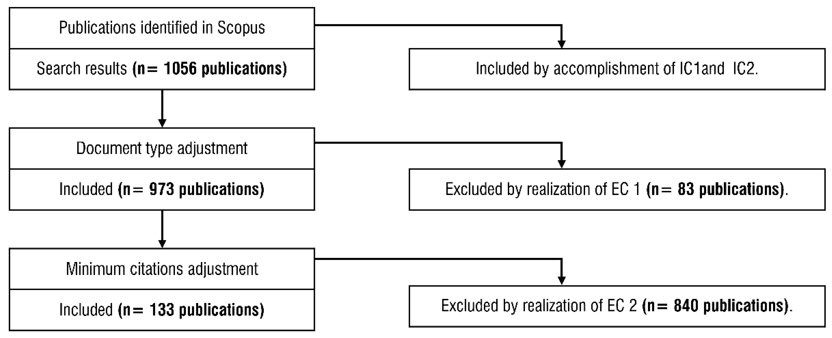
• IC 1. The search string (TITLE-ABS-KEY (hyperspectral AND anomaly AND detection))
• IC 2. The publications are written in English.

The exclusion criteria (EC) define what publications should be discarded from the research collection. In this work, two EC were defined:

• EC 1. Reviews and conference reviews, books and book chapters, letters and notes.
• EC 2. Publications with less than three citations per year.

The first EC resulted in the selection of articles and conference papers that could be seen as the primary sources of scientific contributions, whereas the excluded document types might not have provided sufficiently novel material on the research subject. The second EC served as the relevance criterion, such that only highly-cited publications were selected for final bibliometric analysis. The overall procedure is depicted in Figure 1.

The bibliometric analysis was performed in the programming language R, using the bibliometrix [23] package. Bibliometrix is an open-source R-package that enables comprehensive science mapping analysis [23].

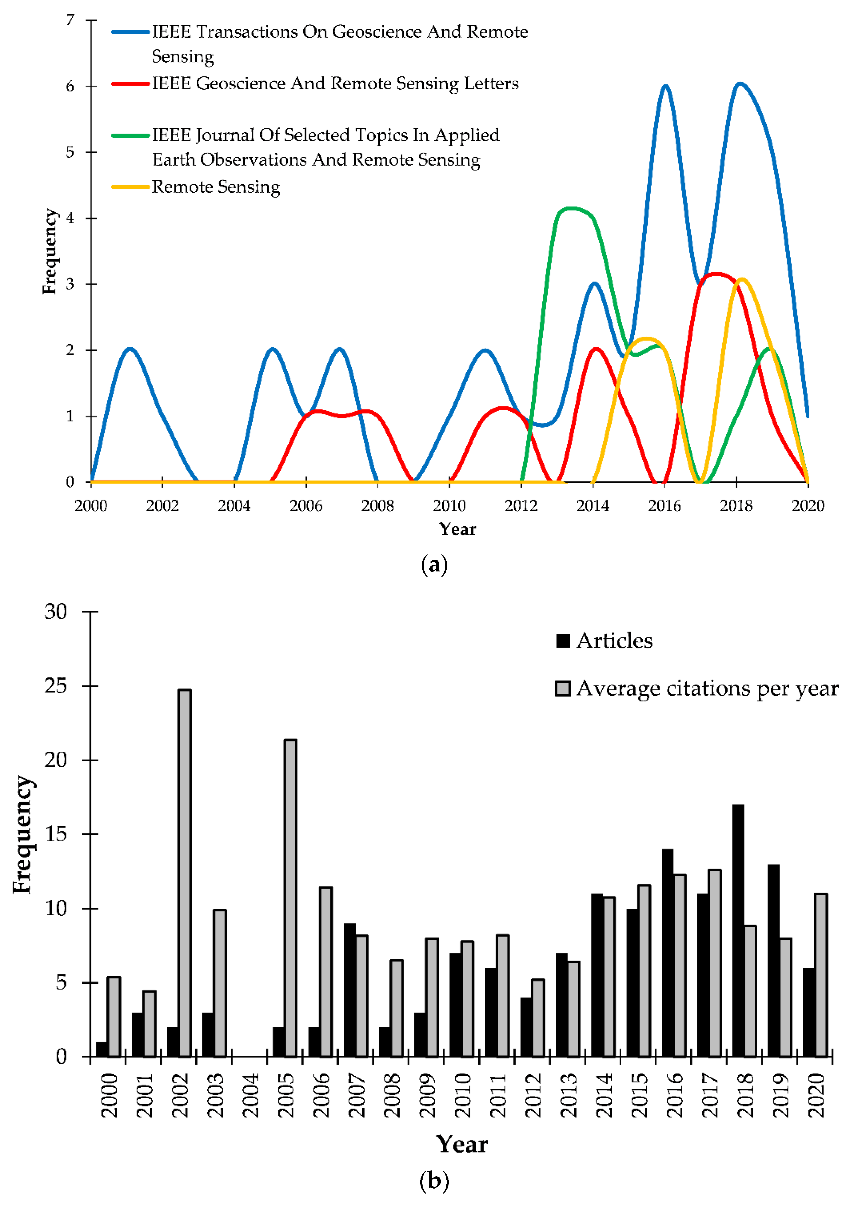
2.1. Descriptive Bibliometric Analysis

The overview of the descriptive bibliometric statistics for the dataset (Figure 1) is presented in

Table 1. Summary bibliometric statistics of the relevant publications on hyperspectral image processing for anomaly detection in remote sensing applications acquired by the presented search strategy (Figure 1).

Main Information	Result
Time span	2000–2020
Sources	41
Total number of documents	133
Average years from publication	7.41
Average citations per documents	72.65
Average citations per year per doc	8.14
References	4276
Document types
Article	118
Conference paper	15
Authors and collaboration
Authors	299
Authors of single-authored documents	5
Authors of multi-authored documents	294
Co-Authors per Documents	3.71
Collaboration Index	2.3

. The search strategy yielded 133 relevant publications on hyperspectral image processing for anomaly detection in remote sensing applications that were published in 41 sources (Table 1). The number of citations per document, on average, was 72.65, or 8.14 citations per document per year, respectively. In the selected publications, a total of 4276 documents were cited. Most publications that fulfilled the search strategy were journal articles (118), with a smaller fraction of conference papers (15). There were only five documents created by a single author, while the average number of co-authors per document was 3.71. In the end, the collaboration index [24] was calculated as the ratio of the total number of authors of multi-authored documents and the total number of multi-authored documents, and scored the value of 2.3.

The core sources of relevant documents, by Bradford’s law [25], were IEEE Transactions On Geoscience And Remote Sensing and IEEE Geoscience And Remote Sensing Letters, which accounted for a total of 54 publications (

Table 2. The most relevant sources (first two zones by Bradford’s law [25]), sorted in descending order by the number of documents.

Rank	Source Name	Documents	Zone 1
1	IEEE Transactions On Geoscience And Remote Sensing	39	1
2	IEEE Geoscience And Remote Sensing Letters	15	1
3	IEEE Journal Of Selected Topics In Applied Earth Observations And Remote Sensing	15	2
4	Remote Sensing	9	2
5	Proceedings Of SPIE - The International Society For Optical Engineering	5	2
6	Remote Sensing Of Environment	3	2
7	Eurasip Journal On Advances In Signal Processing	2	2
8	IEEE Access	2	2

¹ By Bradford’s law [25].

).

The top journal (Table 2) was appreciated among the first publications on this topic, and the appearance of the consequent sources followed their popularity (Figure 2a). The first document was published in the IEEE Geoscience And Remote Sensing Letters (rank 2) in 2005, in the IEEE Journal Of Selected Topics In Applied Earth Observations And Remote Sensing in 2012, and in the Remote Sensing in 2014. Researchers in this scientific field were most productive in 2018 (Figure 2b). However, the articles published in 2002 and 2005 attracted the most attention from the scientific community (Figure 2b).

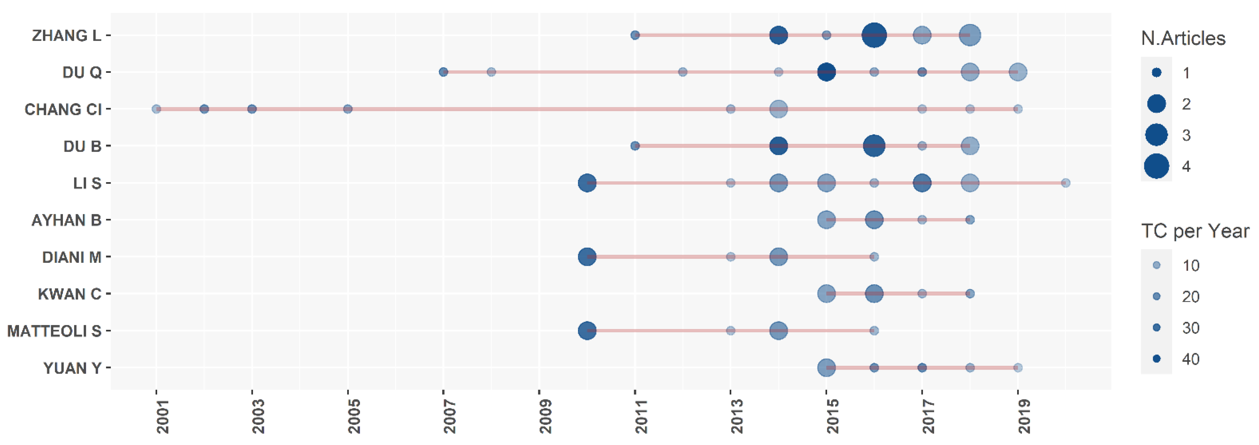
2.2. Authors Analysis

The 20 most relevant authors, sorted by number of total citations and respective bibliometric statistics, are listed in

Table 3. The statistics of the 20 most relevant authors in the topic, sorted by total number of citations.

Author	SCOPUS Author ID	H-index	Total Citations	Number of Publications	First Publication (Year)
Chang CI	35253647700	10	1259	10	2001
Du Q	7202060063	11	1044	12	2007
Zhang L	8359720900	13	962	13	2011
Du B	55020400300	9	799	9	2011
Nasrabadi NM	7006312852	3	724	3	2003
Stocker AD	7006884172	2	698	2	2002
Kwon H	7401838362	3	611	3	2003
Diani M	7003735775	6	597	6	2010
Matteoli S	24076749300	6	597	6	2010
Beaven SG	57206689538	1	554	1	2002
Hoff LE	7005107977	1	554	1	2002
Schaum AP	57207501822	1	554	1	2002
Stein DWJ	7401616297	1	554	1	2002
Winter EM	7102040936	1	554	1	2002
Fowler JE	7402370679	4	513	4	2007
Chiang SS	7201472110	2	511	2	2001
Li J	24481713500	5	496	5	2014
Corsini G	7103074007	5	486	5	2010
Li W	56215159000	4	442	4	2015
Plaza A	7006613644	5	420	5	2010

. Chein-I Chang was the most cited author, with 1259 citations from 10 publications. He was followed by Du Qian with 1044 citations, who was the second most productive author with 12 publications. The most productive author, with 13 publications, was Zhang Liangpei.

Scientific production over the time span of the research (Table 1) for the top 10 authors by number of articles and total number of citations per year is presented in Figure 3. The most cited author has also been the most persistent author in the field, with his first publication originating back in 2001 and the last published in 2019. It is interesting to see that the second most cited author has also been the second most persistent, publishing articles from 2007 to 2019. It can be noticed that some authors listed in Figure 3 are not listed in Table 3, and the reason is that sorting in Figure 3 included the normalization of citations per year. Hence, some authors had recently published quality papers with high citation rates, but the total number of citations was still not high enough to earn them a place in Table 3.

Table 4 and Table 5 contain the top documents measured by global and local citations, respectively. Table 4 relates to the publications that were selected within the search strategy, sorted by global citations. Table 5 refers to documents that were highly cited locally but not enclosed by the search strategy results.

The work of Stein et al. [15] received the highest number of global citations and the second-highest number of local citations. In the analyzed document list (Figure 1), the work of Kwon and Nasrabadi [26] was appreciated the most, but it also attracted significant attention from the general scientific community, with 470 global citations. The more recent work on collaborative representation for hyperspectral anomaly detection by Li and Du [27] should be underlined, as it received great attention, both globally or locally.

Table 4. The top 10 documents with the highest number of global citations.

Document	Reference	Global Citations	Local Citations
Stein, D.W.J.; Beaven, S.G.; Hoff, L.E.; Winter, E.M.; Schaum, A.P.; Stocker, A.D. Anomaly detection from hyperspectral imagery. IEEE Signal Process Mag 2002, 19, 58–69, doi:10.1109/79.974730	[15]	554	54
Kwon, H.; Nasrabadi, N.M. Kernel RX-algorithm: A non-linear anomaly detector for hyperspectral imagery. IEEE Trans Geosci Remote Sens 2005, 43, 388–397, doi:10.1109/TGRS.2004.841487	[26]	470	56
Chang, C.I.; Chiang, S.S. Anomaly detection and classification for hyperspectral imagery. IEEE Trans Geosci Remote Sens 2002, 40, 1314–1325, doi:10.1109/TGRS.2002.800280	[28]	386	51
Ren, H.; Chang, C., I. Automatic spectral target recognition in hyperspectral imagery. IEEE Trans. Aerosp. Electron. Syst. 2003, 39, 1232–1249, doi:10.1109/TAES.2003.1261124.	[29]	360	5
Matteoli, S.; Diani, M.; Corsini, G. A tutorial overview of anomaly detection in hyperspectral images. IEEE Aerosp Electron Syst Mag 2010, 25, 5–27, doi:10.1109/MAES.2010.5546306.	[11]	322	33
Du, Q.; Fowler, J.E. Hyperspectral Image Compression Using JPEG2000 and Principal Component Analysis. IEEE Geoscience and Remote Sensing Letters 2007, 4, 201–205, doi:10.1109/LGRS.2006.888109.	[30]	321	2
Banerjee, A.; Burlina, P.; Diehl, C. A support vector method for anomaly detection in hyperspectral imagery. IEEE Trans Geosci Remote Sens 2006, 44, 2282–2291, doi:10.1109/tgrs.2006.873019.	[31]	286	38
Li, W.; Du, Q. Collaborative representation for hyperspectral anomaly detection. IEEE Trans Geosci Remote Sens 2015, 53, 1463–1474, doi:10.1109/tgrs.2014.2343955.	[27]	251	42
Penna, B.; Tillo, T.; Magli, E.; Olmo, G. Transform Coding Techniques for Lossy Hyperspectral Data Compression. IEEE Trans Geosci Remote Sens 2007, 45, 1408–1421, doi:10.1109/TGRS.2007.894565.	[32]	241	3
Du, B.; Zhang, L. A Discriminative Metric Learning Based Anomaly Detection Method. IEEE Trans Geosci Remote Sens 2014, 52, 6844–6857, doi:10.1109/TGRS.2014.2303895.	[33]	220	27

Table 4. The top 10 documents with the highest number of global citations.

Document	Reference	Global Citations	Local Citations
Stein, D.W.J.; Beaven, S.G.; Hoff, L.E.; Winter, E.M.; Schaum, A.P.; Stocker, A.D. Anomaly detection from hyperspectral imagery. IEEE Signal Process Mag 2002, 19, 58–69, doi:10.1109/79.974730	[15]	554	54
Kwon, H.; Nasrabadi, N.M. Kernel RX-algorithm: A non-linear anomaly detector for hyperspectral imagery. IEEE Trans Geosci Remote Sens 2005, 43, 388–397, doi:10.1109/TGRS.2004.841487	[26]	470	56
Chang, C.I.; Chiang, S.S. Anomaly detection and classification for hyperspectral imagery. IEEE Trans Geosci Remote Sens 2002, 40, 1314–1325, doi:10.1109/TGRS.2002.800280	[28]	386	51
Ren, H.; Chang, C., I. Automatic spectral target recognition in hyperspectral imagery. IEEE Trans. Aerosp. Electron. Syst. 2003, 39, 1232–1249, doi:10.1109/TAES.2003.1261124.	[29]	360	5
Matteoli, S.; Diani, M.; Corsini, G. A tutorial overview of anomaly detection in hyperspectral images. IEEE Aerosp Electron Syst Mag 2010, 25, 5–27, doi:10.1109/MAES.2010.5546306.	[11]	322	33
Du, Q.; Fowler, J.E. Hyperspectral Image Compression Using JPEG2000 and Principal Component Analysis. IEEE Geoscience and Remote Sensing Letters 2007, 4, 201–205, doi:10.1109/LGRS.2006.888109.	[30]	321	2
Banerjee, A.; Burlina, P.; Diehl, C. A support vector method for anomaly detection in hyperspectral imagery. IEEE Trans Geosci Remote Sens 2006, 44, 2282–2291, doi:10.1109/tgrs.2006.873019.	[31]	286	38
Li, W.; Du, Q. Collaborative representation for hyperspectral anomaly detection. IEEE Trans Geosci Remote Sens 2015, 53, 1463–1474, doi:10.1109/tgrs.2014.2343955.	[27]	251	42
Penna, B.; Tillo, T.; Magli, E.; Olmo, G. Transform Coding Techniques for Lossy Hyperspectral Data Compression. IEEE Trans Geosci Remote Sens 2007, 45, 1408–1421, doi:10.1109/TGRS.2007.894565.	[32]	241	3
Du, B.; Zhang, L. A Discriminative Metric Learning Based Anomaly Detection Method. IEEE Trans Geosci Remote Sens 2014, 52, 6844–6857, doi:10.1109/TGRS.2014.2303895.	[33]	220	27

Table 5. The top 10 documents with the highest number of local citations that were not selected within the applied search strategy (Figure 1).

Document	Reference	Local Citations
Reed, I.S.; Yu, X. Adaptive Multiple-Band CFAR Detection of an Optical Pattern with Unknown Spectral Distribution. IEEE Trans. Acoust. Speech Sign. Proces. 1990, 38, 1760–1770, doi:10.1109/29.60107.	[34]	90
Carlotto, M.J. A cluster-based approach for detecting man-made objects and changes in imagery. IEEE Trans Geosci Remote Sens 2005, 43, 374–387, doi:10.1109/TGRS.2004.841481	[35]	32
Manolakis, D.; Shaw, G. Detection algorithms for hyperspectral imaging applications. IEEE Signal Process Mag 2002, 19, 29–43, doi:10.1109/79.974724.	[9]	32
Nasrabadi, N.M. Hyperspectral target detection: An overview of current and future challenges. IEEE Signal Process Mag 2014, 31, 34–44, doi:10.1109/MSP.2013.2278992	[18]	21
Harsanyi, J.C.; Chang, C.I. Hyperspectral Image Classification and Dimensionality Reduction: An Orthogonal Subspace Projection Approach. IEEE Trans Geosci Remote Sens 1994, 32, 779–785, doi:10.1109/36.298007	[36]	19
Kerekes, J. Receiver operating characteristic curve confidence intervals and regions. IEEE Geoscience and Remote Sensing Letters 2008, 5, 251–255, doi:10.1109/lgrs.2008.915928.	[37]	17
Manolakis, D.; Marden, D.; Shaw, G.A. Hyperspectral Image Processing for Automatic Target Detection Applications. Lincoln laboratory journal 2003, 14, 79–116	[38]	16
Nasrabadi, N.M. Regularization for spectral matched filter and RX anomaly detector. In Proceedings of Proc SPIE Int Soc Opt Eng, 2008	[39]	16
Chen, Y.; Nasrabadi, N.M.; Tran, T.D. Sparse Representation for Target Detection in Hyperspectral Imagery. IEEE J. Sel. Top. Signal Process. 2011, 5, 629–640, doi:10.1109/jstsp.2011.2113170	[40]	16
Chen, Y.; Nasrabadi, N.M.; Tran, T.D. Hyperspectral Image Classification Using Dictionary-Based Sparse Representation. IEEE Trans Geosci Remote Sens 2011, 49, 3973–3985, doi:10.1109/tgrs.2011.2129595.	[41]	16

Table 5. The top 10 documents with the highest number of local citations that were not selected within the applied search strategy (Figure 1).

Document	Reference	Local Citations
Reed, I.S.; Yu, X. Adaptive Multiple-Band CFAR Detection of an Optical Pattern with Unknown Spectral Distribution. IEEE Trans. Acoust. Speech Sign. Proces. 1990, 38, 1760–1770, doi:10.1109/29.60107.	[34]	90
Carlotto, M.J. A cluster-based approach for detecting man-made objects and changes in imagery. IEEE Trans Geosci Remote Sens 2005, 43, 374–387, doi:10.1109/TGRS.2004.841481	[35]	32
Manolakis, D.; Shaw, G. Detection algorithms for hyperspectral imaging applications. IEEE Signal Process Mag 2002, 19, 29–43, doi:10.1109/79.974724.	[9]	32
Nasrabadi, N.M. Hyperspectral target detection: An overview of current and future challenges. IEEE Signal Process Mag 2014, 31, 34–44, doi:10.1109/MSP.2013.2278992	[18]	21
Harsanyi, J.C.; Chang, C.I. Hyperspectral Image Classification and Dimensionality Reduction: An Orthogonal Subspace Projection Approach. IEEE Trans Geosci Remote Sens 1994, 32, 779–785, doi:10.1109/36.298007	[36]	19
Kerekes, J. Receiver operating characteristic curve confidence intervals and regions. IEEE Geoscience and Remote Sensing Letters 2008, 5, 251–255, doi:10.1109/lgrs.2008.915928.	[37]	17
Manolakis, D.; Marden, D.; Shaw, G.A. Hyperspectral Image Processing for Automatic Target Detection Applications. Lincoln laboratory journal 2003, 14, 79–116	[38]	16
Nasrabadi, N.M. Regularization for spectral matched filter and RX anomaly detector. In Proceedings of Proc SPIE Int Soc Opt Eng, 2008	[39]	16
Chen, Y.; Nasrabadi, N.M.; Tran, T.D. Sparse Representation for Target Detection in Hyperspectral Imagery. IEEE J. Sel. Top. Signal Process. 2011, 5, 629–640, doi:10.1109/jstsp.2011.2113170	[40]	16
Chen, Y.; Nasrabadi, N.M.; Tran, T.D. Hyperspectral Image Classification Using Dictionary-Based Sparse Representation. IEEE Trans Geosci Remote Sens 2011, 49, 3973–3985, doi:10.1109/tgrs.2011.2129595.	[41]	16

Although the search strategy did not cover it, the paper published in 1990 by Reed and Yu [34] received by far the highest number of local citations. In that paper, the foundations of the well-known (Reed-Xiaoli, RX) hyperspectral anomaly detector were established. This algorithm is still popular; it is widely regarded as the benchmark hyperspectral anomaly detection technique and is often used in the comparison of newly developed anomaly detectors.

Manolakis and Shaw (Table 5) are among the pioneers of hyperspectral target and anomaly detection, and their work is also highly cited. The diligent work of Nasrabadi has been recognized, accounting for as many as four out of the 10 top locally cited publications in Table 5.

Figure 4 and

Table 6. The topic development expressed by the key author’s keywords over time. The most relevant keywords were filtered and manually selected by authors.

Year	Document
2001	Competitive Region Growth, Elliptically Contoured Distributions, Evolutional Algorithm, Kurtosis, Projection Pursuit, Spherically Invariant Random Vectors
2002	Causal RXD, Correlation Matched-Filter-Based Measure, Target Discrimination Measure
2003	Clustering Algorithms, Dual Window, Eigen Separation Transform, Embedded Computing
2005	Kernels, Linear Discriminant Analysis, Orthogonal Subspace Projection/AD, RX Detector, Signal Parameter Estimation
2006	Bhattacharyya Distance, Signal Subspace Processing, Support Vector Data Description (SVDD)
2007	Detection Index, Minimum Description Length, Real-Time (R-T) Processing, Self-Organising Maps, Separability Index, Signal-Subspace Rank, Singular Value Decomposition, Wavelets
2008	Karhunen-Love-Transform, Principal Component Analysis (PCA), Kernel PCA, Signal Detection, Spectral Decorrelation
2009	GPU Processing, Generalized Least Squares, Maximum Autocorrelation Factors, Multivariate Normal Mixture Model, Principal Autocorrelation Factors
2010	Cluster-Based Approach, Feature Selection, Kernel-Based Learning, Quasi-Local Covariance Matrix, Regularization, Robust Locally Linear Embedding
2011	Embedded Systems, Gaussian Kernel, Independent Component Analysis, ROC Space, Sparse Matrix Transform, Support vector machine (SVM)
2012	Clustering, Compressed Sensing, PCA, Segmentation-Based AD, Sparse Kernel-Based Ensemble Learning, Spectral Unmixing
2013	Bayesian Learning, Dual Window-Based Eigen Separation Transform, Finite Mixture Model, Kernel density estimation (KDE), Multicore Platforms, Multiple-Window AD, Nonlinear PCA
2014	Dimensionality Reduction, High-Order Statistics, Local Sparsity Divergence, Low-Rank (L-R) And Sparse, Matched Filter, Robust Regression Analysis, Superpixels, Variable Bandwidth KDE, Weighted-RXD
2015	Graph Theory, High Order Statistics, L-R Approximation, Manifold Learning, R-T processing, Residual Analysis, Robust Background Estimation
2016	Cluster Kernel RX, Dual Clustering, Kernel Collaborative Representation (CR), Local Summation Strategy, Locally Linear Embedding, ROC, Robust PCA, Sparse Representation (SR), Sparsity Divergence Index, Spectral-Spatial Integration, Tensor Representation
2017	3-D ROC, Band Subset Selection, Convolutional Neural Network (NN), Differential Morphology, Edge-Preserving Filtering, Joint SR, K-SVD, Multiple Graphs, Autoencoders, Tensor Decomposition
2018	A Posteriori AD, Band Selection, Deep Learning, Feature Extraction, Inverse PCA, Iterative AD, L-R Representation, Multiple Dictionaries, R-T Applications, Sparse Coding, Structured SR
2019	Adaptive Weighting, Constrained SR, Deep Brief Network, Dictionary Learning, Fractional Fourier, Local Summation, Low Dimensional Manifold Model, Structure Tensor
2020	Density Peak Clustering, Isolation Forest, Radiative Transfer Modeling

depict the temporal development of research on hyperspectral image processing for anomaly detection in remote sensing applications. Table 6 is based on the use of the author’s keywords, and Figure 4, on the document title’s keywords. In selecting the author’s keywords presented in Table 6, trivial keywords such as hyperspectral, anomaly, detection, target, background, and similar terms were omitted. Then, the most relevant keywords were manually selected from the remaining keywords based on keyword frequency and global citation of the respective document. For the creation of Figure 4, the most frequent title keywords per year are displayed with the constraint of a maximum of three keywords per year. The respective frequency (for the specific year) is displayed on a vertical axis in a logarithmic scale, and as can be seen, no trivial keywords were omitted, nor was any manual filtering performed.

The Word cloud presented in Figure 5 enables clear insight into the trends and future scientific research in hyperspectral image processing for anomaly detection in remote sensing applications. The figure was generated using the document title keywords, similarly as in Figure 4, but here, the total frequency over the analyzed time span was considered. The total frequencies determined the respective size of words, so the most frequent keywords were written with more prominent characters.

By analyzing Figure 4 and Figure 5 and Table 6, a recent trend in the development of representation-based techniques can be identified. Low-rank, spare, collaboration, joint, and dictionary are terms that can be related to these techniques. Hence, a special section is dedicated to these methods in Part B of this paper.

3. Part B: An Overview of Hyperspectral Image Processing for Anomaly Detection in Remote Sensing Applications

This section provides a mathematical framework for anomaly detection, followed by the description of specific anomaly detection techniques that are generally divided into methods that adopt structured background models or unstructured background models.

4. Mathematical Framework for Anomaly Detection

The mathematical framework for anomaly detection arises from the signal detection theory [42], and is based on the field of statistical or binary hypothesis testing. A hyperspectral image or a hyperspectral cube can be regarded as a rank-3 tensor arranged in two spatial dimensions and one spectral dimension. If we consider a hyperspectral cube having N pixels and $K$ spectral bands ($\underset{\_}{\underset{\_}{X}}\in {ℝ}^{N\times K}$), then a pixel spectrum could be represented as the realization of a random vector ($\underset{\_}{X}$) that can be denoted as $\underset{\_}{x}={\left[x_1, x_2,\dots ,x_K \right]}^T$. Given an observed pixel $\underset{\_}{x}$, it needs to be decided between two disjunct premises:

$$\widehat{H}\left(\underset{\_}{x}\right)=\{\begin{array}{c}{H}_0: \mathrm{target} \mathrm{absent} \left( \underset{\_}{x} \mathrm{is} \mathrm{a} \mathrm{background} \mathrm{pixel} \right) \\ H_1: \mathrm{target} \mathrm{present} \left( \underset{\_}{x} \mathrm{is} \mathrm{a} \mathrm{target} \mathrm{pixel} \right) \end{array}.$$

(1)

In general, a statistical hypothesis test is a rule for division of input $K$-dimensional feature space in two segments: space $\left(A\right)$ consistent with the null hypothesis $H_0$ and its complement (B) that contains values consistent with the alternative hypothesis $H_1$. In signal detection theory terminology, it can be stated that a decision about the proper hypothesis is determined by a test or detection statistic ($\Lambda , \Lambda \left(\underset{\_}{x}\right)=\lambda$) whose detection threshold or critical value ($\eta$) splits input feature space into segments A ($H_0:\Lambda \left(\underset{\_}{x}\right)\le \eta$) and B ($H_1:\Lambda \left(\underset{\_}{x}\right)>\eta$). The detection statistic usually maps input n-dimensional feature space ($K$-dimensional in our specific case) into 1-dimensional space, thus enabling separation of spaces $A$ and B on a line instead of some high dimensional space.

Upon hypothesis testing, two types of erroneous inferences could arise: a type I error occurs if a null hypothesis $H_0$ is rejected while being true, and a type II error occurs if the $H_0$ is accepted when the alternative hypothesis $H_1$ is true. The probability of a type I error is usually denoted with α, commonly called the significance level. It can be mathematically formulated as [11]:

$$\alpha =P\left\{\Lambda \left(\underset{\_}{x}\right)>\eta |H_0\right\}={\int }_{\lambda >\eta }{f}_{\Lambda |H_0}\left(\lambda \right)d\lambda ={\int }_{\underset{\_}{x}:\Lambda \left(\underset{\_}{x}\right)>\eta }{f}_{\underset{\_}{X}|H_0}\left(\underset{\_}{x}\right)d\underset{\_}{x}.$$

(2)

In hyperspectral anomaly detection, a type I error occurs if an observed pixel is proclaimed as a target (anomaly) when it actually belongs to the background. Therefore, a type I error is also called a false alarm ($P_{FA}=\alpha$). The probability of a type II error is usually denoted with β, and it can be expressed as [11]:

$$\beta =P\left\{\Lambda \left(\underset{\_}{x}\right)\le \eta |H_1\right\}={\int }_{\lambda \le \eta }{f}_{\Lambda |H_1}\left(\lambda \right)d\lambda ={\int }_{\underset{\_}{x}:\Lambda \left(\underset{\_}{x}\right)\le \eta }{f}_{\underset{\_}{X}|H_1}\left(\underset{\_}{x}\right)d\underset{\_}{x}.$$

(3)

A type II error happens if an observed pixel is proclaimed as a background pixel when it is a target (anomaly), thus resulting in missed detection. When β is known, the probability of anomaly detection ($P_D)$ can be directly determined as in [11]:

$$\begin{array}{c}{P}_D=1-\beta \\ P_D=P\left\{\Lambda \left(\underset{\_}{x}\right)>\eta |H_1\right\}={\int }_{\lambda >\eta }{f}_{\Lambda |H_1}\left(\lambda \right)d\lambda ={\int }_{\underset{\_}{x}:\Lambda \left(\underset{\_}{x}\right)>\eta }{f}_{\underset{\_}{X}|H_1}\left(\underset{\_}{x}\right)d\underset{\_}{x}\end{array}.$$

(4)

The ideal detection statistic could make the probabilities of both error types arbitrarily small, but no such statistical test exists. In statistical decision theory, it is well-accepted that decisions based on the likelihood ratio test (LRT) are optimum over numerous performance criteria [10,42]. Let$f(\underset{\_}{X}|H_0)$ and $f(\underset{\_}{X}|H_1)$ be conditional probability distributions of observing $\underset{\_}{x}$ under $H_0$ and $H_1$ respectively. Then, the LRT between $(\underset{\_}{X}|H_0)$ and $f(\underset{\_}{X}|H_1)$ can be derived as [10]:

$$\Lambda \left(\underset{\_}{x}\right)=\frac{f_{\underset{\_}{X}|H_1}\left(\underset{\_}{x}\right)}{f_{\underset{\_}{X}|H_0}\left(\underset{\_}{x}\right)} \begin{array}{c}{H}_1\\ >\\ <\\ H_0\end{array} \eta .$$

(5)

The classical approach in selecting optimum detection statistics is based on the well-known Neyman-Pearson (NP) lemma [43]. The NP lemma for a given significance level $\alpha$ obtains the test that has the lowest possible probability of missed detection β for all parameters defined by the alternative hypothesis $H_1$. In other words, NP is the optimum criterion that maximizes the probability of detection for any desired false alarm rate [42]. Solution of (5), in an NP sense, is only possible if both hypothesis $H_0$ and $H_1$ are simple hypotheses. Simple hypotheses have parameters of their conditional probability functions $f(\underset{\_}{X}|H_0)$ and $f(\underset{\_}{X}|H_1)$ known, but unfortunately, these requirements are rarely fulfilled in practical applications. In those cases, sub-optimum criteria that are based on the generalized likelihood ratio test (GLRT) are implemented. In GLRTs, unknown parameters are substituted with their maximum likelihood estimates (MLE) [11,38]:

$${\Lambda }_{GLRT}\left(\underset{\_}{x}\right)=\frac{f_{\underset{\_}{X}|H_1}(\underset{\_}{x};{\widehat{\underset{\_}{\vartheta }}}_1)}{ f_{\underset{\_}{X}|H_0}(\underset{\_}{x};{\widehat{\underset{\_}{\vartheta }}}_0)}=\frac{ma{x}_{{\underset{\_}{\vartheta }}_1} f_{\underset{\_}{X}|H_1}(\underset{\_}{x};{\widehat{\underset{\_}{\vartheta }}}_1)}{ma{x}_{{\underset{\_}{\vartheta }}_0} f_{\underset{\_}{X}|H_0}(\underset{\_}{x};{\widehat{\underset{\_}{\vartheta }}}_0)} \begin{array}{c}{H}_1\\ >\\ <\\ H_0\end{array} \eta ,$$

(6)

where ${\widehat{\underset{\_}{\vartheta }}}_0,$ ${\widehat{\underset{\_}{\vartheta }}}_1$ represent the vectors of unknown parameters. MLEs of unknown parameters are usually determined from the test and/or reference samples that should be independent and identically distributed (IID).

In anomaly detection, no presumptions about the target model are made. Instead, background models are developed. In doing so, a wide variety of creative approaches were suggested, including the adoption of multivariate normal models [34], subspace projections [36], and kernel methods [26]. Although attempts have been made to provide the in-depth taxonomy of complex hyperspectral anomaly detection methods [10,11] or background modeling for detection of anomalies in hyperspectral remotely sensed imagery [17], we suggest a simple distinction of anomaly detection methods in two basic categories: methods that implement unstructured background models and methods that adopt structured background models.

Besides background models, methods could be further specified by the implemented spatial model. The spatial model can be one of the following: global, local, or quasi-local. If a global model is used, then all or most available hyperspectral pixels are used to characterize the background. In a local model, only the spatial neighbors of PUT are used for the description of the background. Quasi-local methods present a trade-off solution to global and local models.

5. Unstructured Background Models

Fundamental anomaly detection methods implement unstructured background models. They are often specified as data-driven, statistical, or probabilistic. These models do not assume any specific structure on the hyperspectral cubes based on a-priori knowledge, but integrate additive noise in the model.

Let $\underset{\_}{\mu }=\left[{\mu }_1,{\mu }_2, \cdots , {\mu }_K\right]$ be the mean vector of a hyperspectral cube with K bands, where ${\mu }_1$ represents the average of all pixels in the first spectral band and ${\mu }_K$ the average of the last spectral band. The mean vector $\underset{\_}{\mu }$ is often called the background centroid or background prototype. In this respect, a squared Euclidean distance between PUT ($\underset{\_}{x}$) and background centroid can be used as a simple detection statistic:

$$d_E^2(\underset{\_}{x},\underset{\_}{\mu })={\left(\underset{\_}{x}-\underset{\_}{\mu }\right)}^T·\left(\underset{\_}{x}-\underset{\_}{\mu }\right).$$

(7)

In hyperspectral images, due to their fine spectral resolution, spectral adjacent bands are usually highly correlated. Therefore in (7), a weighting matrix in the form of the inverse covariance matrix (${\underset{\_}{\underset{\_}{\Gamma }}}^{-1}$) could be added:

$$d_M^2(\underset{\_}{x},\underset{\_}{\mu })={\left(\underset{\_}{x}-\underset{\_}{\mu }\right)}^T·{\underset{\_}{\underset{\_}{\Gamma }}}^{-1}·\left(\underset{\_}{x}-\underset{\_}{\mu }\right).$$

(8)

Expression (8) represents the widely known squared Mahalanobis distance [44] between PUT and background centroid. It should be noticed that distance in (8) is proportional with negative log-likelihood of Gaussian or normal distribution:

$$d_M\left(\underset{\_}{x},\underset{\_}{\mu }\right)\propto -\log p_{\mathcal{N}}(\underset{\_}{x}|\underset{\_}{\mu },\underset{\_}{\underset{\_}{\Gamma }}),$$

(9)

where

$$p_{\mathcal{N}}(\underset{\_}{x}|\underset{\_}{\mu },\underset{\_}{\underset{\_}{\Gamma }})=\frac{1}{{\left(2\pi \right)}^{\frac{\mathrm{K}}{2}}·{\left|\underset{\_}{\underset{\_}{\Gamma }}\right|}^{\frac{1}{2}}}exp\left(-\frac{1}{2}{\left(\underset{\_}{x}-\underset{\_}{\mu }\right)}^{\mathrm{T}}·{\underset{\_}{\underset{\_}{\Gamma }}}^{-1}·\left(\underset{\_}{x}-\underset{\_}{\mu }\right)\right).$$

(10)

Therefore, if a background can be adequately characterized with the multivariate normal distribution, then the squared Mahalanobis distance could be an appropriate detection statistic for anomaly detection. The multivariate normal model for anomaly detection can be written as:

$$\begin{array}{l}\underset{\_}{X}|H_0=\underset{\_}{B} \hspace{1em}\in \mathcal{N}\left(\underset{\_}{\mu },\underset{\_}{\underset{\_}{\Gamma }}\right)\\ \underset{\_}{X}|H_1=\underset{\_}{s}+\underset{\_}{B} \hspace{1em}\in \mathcal{N}\left(\underset{\_}{s},\underset{\_}{\underset{\_}{\Gamma }}\right)\end{array},$$

(11)

where $\underset{\_}{B}$ denotes the spectral vector belonging to the background (which incorporates additive noise), $\underset{\_}{s}$ is the spectral vector of the target, and $\underset{\_}{\underset{\_}{\Gamma }}$ is the background covariance matrix that is assumed to be the same for the background and target class. The most popular anomaly detector for hyperspectral remote sensed images is based on the multivariate normal model, and it is named the Reed-Xiaoli (RX) algorithm [34].

5.1. Reed-Xiaoli (RX) Algorithm

The RX algorithm [34] can be considered as the reference in hyperspectral image processing for anomaly detection in remote sensing applications, and it has become the standard with which new anomaly detectors are compared [45,46,47,48,49]. The algorithm idea stemmed from the test developed for the detection of radar targets [50], as well as most of the detection theory in remote sensing that arose from the processing of radar data. RX is an adaptive constant false alarm rate (CFAR) hyperspectral anomaly detection algorithm developed from the GLRT [34]. CFAR algorithms exhibit the property that the probability of false alarm does not depend on any unknown parameter, and it is a highly desirable property in the design of anomaly detectors. It should be noticed that in (11) the covariance matrices for background and target class are assumed to be the same. This condition needs to be fulfilled in order to make the RX detector optimum in a Neyman-Pearson sense (5), i.e., to hold the CFAR property [38].

To date, many implementations of the RX algorithm have been proposed: global, local, and quasi-local. Although RX in its original form is a local algorithm, we will describe its global variant first as it is the simplest one. The local and quasi-local RX models will follow afterward.

Hyperspectral pixels are considered as random spectral vectors that are IID. These pixels are then used for estimation of unknown parameters of the multivariate normal distribution: $\underset{\_}{\mu }$ and $\underset{\_}{\underset{\_}{\Gamma }}$. Consider a hyperspectral cube with a total of N pixels, namely N random spectral vectors with K elements (K being the number of spectral bands). The global RX detector can be defined as [34]:

$$D_{RX}(\underset{\_}{x}|ℬ)=D_{RX}(\underset{\_}{x}|\underset{\_}{B})={\left(\underset{\_}{x}-\underset{\_}{\widehat{\mu }}\right)}^T·{\underset{\_}{\underset{\_}{\widehat{\Gamma }}}}^{-1}·\left(\underset{\_}{x}-\underset{\_}{\widehat{\mu }}\right)\begin{array}{c}{H}_1\\ >\\ <\\ H_0\end{array} \lambda ,$$

(12)

where $ℬ$ represents the theoretical background model, while MLEs $\underset{\_}{\widehat{\mu }}$ and $\underset{\_}{\underset{\_}{\widehat{\Gamma }}}$ are determined as:

$$\begin{array}{c}\widehat{\underset{\_}{\mu }}=\frac{1}{N}\sum _{i=1}^N{\underset{\_}{x}}_i\\ \underset{\_}{\underset{\_}{\widehat{\Gamma }}}=\frac{1}{N-1}{\displaystyle \sum }_{i=1}^N\left({\underset{\_}{x}}_i-\widehat{\underset{\_}{\mu }}\right)·{\left({\underset{\_}{x}}_i-\widehat{\underset{\_}{\mu }}\right)}^T\end{array}.$$

(13)

Theoretical foundations for the local (and native) RX detector were set by Hunt and Cannon [51]. They suggested that an optical digital image can be modeled as a nonstationary multivariate Gaussian random process with a highly space-varying spatially nonstationary mean vector and spatially stationary or much less space-varying covariance matrix. The local RX detector uses the same mathematical methodology as the global RX, though it calculates the MLE of unknown parameters (13) using the selected pixels found in the PUT’s spatial neighborhood (Figure 6). The local neighborhood is usually defined using one or more sliding windows (annulus). There are various strategies in selecting the number of windows and their sizes. If only one window is used, it presents an outer window used to estimate all unknown parameters. The most accepted strategy includes the use of three distinct windows: guard window and windows for estimation of $\widehat{\underset{\_}{\mu }}$ and $\underset{\_}{\underset{\_}{\widehat{\Gamma }}}$, with their respective sizes (expressed in widths) $w_g$, $w_{\widehat{\underset{\_}{\mu }}}$ and $w_{\underset{\_}{\underset{\_}{\widehat{\Gamma }}}}$ (Figure 6). The guard window is the smallest window, and it defines the area from which samples are not taken, as there is a possibility that it contains pixels that could be anomalies or pixels that are spectral mixtures with anomalies. Inclusion of these pixels in the calculation of $\widehat{\underset{\_}{\mu }}$ and $\underset{\_}{\underset{\_}{\widehat{\Gamma }}}$ would lead to lower anomaly detection statistic scores and finally decrease the probability of detection. Therefore, its size should be set to accommodate for expected target sizes. Windows for $\widehat{\underset{\_}{\mu }}$ and $\underset{\_}{\underset{\_}{\widehat{\Gamma }}}$, defined as hollow boxes bounded with guard window from the inside are used for estimation of $\widehat{\underset{\_}{\mu }}$ and $\underset{\_}{\underset{\_}{\widehat{\Gamma }}}$. It was shown in [52,53] that local Gaussianity on the image can be forced by subtracting the nonstationary mean. In [34], it is suggested that residual background is a zero-mean Gaussian and independent in spatial domain:

$$\begin{array}{c}\underset{\_}{X}|H_0=\underset{\_}{B} \in \mathcal{N}\left(\underset{\_}{0},\widehat{\underset{\_}{\underset{\_}{\Gamma }}}\right)\\ \underset{\_}{X}|H_1=\underset{\_}{s}+\underset{\_}{B} \in \mathcal{N}\left(\underset{\_}{s},\widehat{\underset{\_}{\underset{\_}{\Gamma }}}\right)\end{array}.$$

(14)

The difference in window sizes for $\widehat{\underset{\_}{\mu }}$ and $\underset{\_}{\underset{\_}{\widehat{\Gamma }}}$ arises from the stationarity of these unknown parameters [51]; the mean should vary more frequently than the covariance matrix.

In selecting the largest window size, a balance between two opposing requirements should be found. The window for $\underset{\_}{\underset{\_}{\widehat{\Gamma }}}$ should include enough samples for stable determination of the inverse of the covariance matrix. Swain and Davis [54] argue that a reliable estimate of covariance matrix requires at least 10 times and preferably 100 times more samples than the number of spectral bands in a hyperspectral image. The opposing requirement states that the window size should be as small as possible to capture a homogenous background and reduce the computational load needed for inverse calculation of the covariance matrix.

Quasi-local implementation of the RX detector includes the use of one global covariance matrix but performs local demeaning. This approach requires the calculation of only one covariance matrix using all available samples, which leads to a more stable inverse and lower computational complexity than the local implementation of the RX detector.

Advantages of the global RX detector are simple implementation and fast computation, as there is only one covariance matrix to be inverted. If the assumptions about the local multivariate normal model (14) and ${\underset{\_}{\underset{\_}{\Gamma }}}_B={\underset{\_}{\underset{\_}{\Gamma }}}_s=\underset{\_}{\underset{\_}{\Gamma }}$ are fulfilled, then the squared Mahalanobis distance follows a non-central chi-squared distribution ${\chi }_K^2\left(\beta \right)$ with K degrees of freedom and non-centrality parameter $\beta$ [38]:

$$D_{RX}(\underset{\_}{x}|ℬ)~\{\begin{array}{c}{\chi }_K^2\left(0\right), under H_0\\ {\chi }_K^2\left(d_M^2\right), under H_1\end{array},$$

(15)

thereby enabling the CFAR property.

The limitation of the local RX detector is that the covariance matrix is determined from a small number of high-dimensional and highly correlated samples. That can result in rank deficiency of covariance matrix or often leads to instability of its inverse. Matrix inversion needs to be calculated for every pixel, which makes the local RX detector computationally intensive. The local RX detector suffers from an increased number of false alarms because some pixels can be anomalies in the local background but not on the entire image (e.g., isolated tree). The main limitation of RX detectors is that in hyperspectral imaging in remote sensing applications, the assumption of Gaussianity is often violated due to the presence of multiple materials in the scene or in the local background, which adversely impacts detection performance.

Improved Variants of the RX Detector

Many authors have tried to tackle the outlined shortcomings of the RX detector and improve its detection performance. First of all, it should be remarked that there is a confounding aspect to the naming of the new anomaly detectors. In our opinion, the RX detector should only refer to the local algorithm defined and explained above, with the exceptions of the global and quasi-local spatial implementations. The anomaly detection methods that use the squared Mahalanobis distance as detection statistics are often named RX variants [15,18,26].

To mitigate the computational cost of the (local) RX detector, a variety of parallel implementations for multicore platforms (CPU and GPU) have been developed [55,56,57,58]. Molero et al. [57] proposed optimized versions of the RX detectors based on the Cholesky decomposition of the correlation matrices with parallel implementations on high-performance computing platforms: multicore and GPU.

Manolakis [10] stated that the normal distribution model accurately fits the body of the data but not its tails. That is particularly important in anomaly detection, as the distribution tails have the most influence on the false alarms. Therefore, the family of multivariate elliptically contoured t distribution, which can model heavier distribution tails, is suggested in lieu of the multivariate normal distribution [59,60,61].

The quasi-local (QL) RX detector is a compromise between the local and global RX detector and should not be confused with the quasi-local implementation of the RX detector. The original QL idea was applied to achieve the QL covariance matrix [62,63,64], but in later publications, this approach is referred to as the QL RX detector [65,66]. The basic idea of the QL RX detector is to decompose the global covariance matrix using the eigenvalue decomposition:

$$\underset{\_}{\underset{\_}{\Gamma }}=\underset{\_}{\underset{\_}{E}}·\underset{\_}{\underset{\_}{\Lambda }}·{\underset{\_}{\underset{\_}{E}}}^T.$$

(16)

The eigenvectors in the $\underset{\_}{\underset{\_}{E}}$ are forwarded to the detector, but the eigenvalues in the $\underset{\_}{\underset{\_}{\Lambda }}$ are replaced by the larger of the local and the global variance [62]:

$${\lambda }_{QL}^i=max\left({\lambda }_{LOCAL}^i,{\lambda }_{GLOBAL}^i\right).$$

(17)

That enables lower detection scores in the image areas with higher variance, and it thus may lead to a lower probability of false alarms. The main benefits of the QL approach are a more stable estimation of the covariance matrix and a much less expensive way of computing its inverse.

Due to the high correlation of the spectral bands, the high dimensionality of the hyperspectral data, and a limited number of samples for estimation of the local covariance matrices, they often suffer from ill-conditioning. A widely accepted method for improving the estimation of the inverse covariance matrix issue is shrinkage [67,68,69,70]. The most straightforward method for the shrinkage of the covariance is the addition of a scaled identity matrix, which is often applied in the ridge regression technique [71]. The ridge regularized (RR) squared Mahalanobis distance (SMD) detector is then formulated as [39]:

$$D_{RR SMD}\left(\underset{\_}{x}|ℬ\right)=d_{M RR}^2\left(\underset{\_}{x},\underset{\_}{\widehat{\mu }}\right)={\left(\underset{\_}{x}-\underset{\_}{\widehat{\mu }}\right)}^T·{\left(\underset{\_}{\underset{\_}{\widehat{\Gamma }}}+\delta \underset{\_}{\underset{\_}{I}}\right)}^{-1}·\left(\underset{\_}{x}-\underset{\_}{\widehat{\mu }}\right)\begin{array}{c}{H}_1\\ >\\ <\\ H_0\end{array} \lambda ,$$

(18)

where $\delta$ denotes the regularization parameter and $\underset{\_}{\underset{\_}{I}}$ is the identity matrix. The same detector (18) is referred to as ridge-regularized RX in [18]. Shrinkage performs small perturbations of the estimated covariance matrix, but that can accomplish significant effects on the invertibility if $\underset{\_}{\underset{\_}{\widehat{\Gamma }}}$ is near-singular. Many other methods for shrinkage can be found in the literature [39,72,73].

Chang and Chiang [28] presented the causal RX detector, which incorporates a sample correlation matrix instead of a covariance matrix and enables real-time processing of the RX detector. In the context of [28], real-time processing refers to processing the pixel as it is received, i.e., in an online data processing approach. Davidson and Ben-David [74] argued for the use of covariance or the correlation matrix and determined that the use of the correlation matrix could offer an improvement over the covariance matrix, but only in a relatively small part of the parameter space. They concluded that the potential performance gain could be modest, yet the potential performance loss could be devastating.

Real-time processing with the RX algorithm has preoccupied numerous scientists [28,75,76,77]. To the best of our knowledge, the first operational implementation of real-time hyperspectral detection was executed in Dark HORSE 1 (Hyperspectral Overhead Reconnaissance and Surveillance Experiment 1) [77]. In that research, it was shown that it is possible to autonomously detect military ground targets using visible hyperspectral images in real-time. In [75], the Woodbury matrix identity is introduced, which could be used to update the previously computed inverse matrix when new data needs to be considered.

To deal with different anomaly sizes, Liu et Chang [78] proposed a multiple-window approach. If the anomalies come in various sizes, as can happen in real applications, the detection performance of the local RX detector is limited. Although the idea is presented in general form, they proposed three specific multiple-window anomaly detectors (MW AD), of which one is the MW variant of RX detector MW-RXD. MW-RXD basically corresponds to the result of the local RX detector that is executed with K different window sizes. Finally, an overall MW-RXD detection map is obtained by a fusion of K detection maps, i.e., a summation of the K local RX detector results [72]:

$$D_{MW-RXD}\left(\underset{\_}{x}|ℬ\right)=\underset{1\le i\le K}{\max }{D}_{RX}{(\underset{\_}{x}|ℬ)}_i.$$

(19)

In [79], a superpixel-based dual window RX (SPDW RX) detector is presented to address the same issue. The SPDW RX uses superpixel segmentation to adaptively determine the dual windows, instead of the two fixed-size windows of the local RX detector. Firstly, the hyperspectral image is divided into superpixels. Then for every superpixel, a minimum bounding rectangle is defined. The background statistics are then determined based on these minimum bounding rectangles, which are further used to calculate the detection statistic. The authors showed that SPDW RX could provide a small increase in detection performance but a large increase in processing speed compared to the local RX detector.

5.2. Nearest Neighbor Detectors

Besides the family of the RX detectors, the detectors based on the principle of the spectrally nearest neighbors (NN) [80,81] can be categorized as the unstructured background anomaly detectors. For the background characterization, a spectral distance of PUT to the C-nearest neighbor can be used as a detection statistic, an average distance of the PUT to the C-nearest neighbors, or a distance of the PUT to the average of the C-nearest neighbors [82]. A choice between various distance metrics could be made: Euclidean, Mahalanobis, spectral angle [83], Manhattan [84], or Chebyshev [85].

The basic NN anomaly detector can be mathematically formulated as follows. Let $w_i$ be the weight, which depends on the distance from the PUT $\underset{\_}{x}$ and background spectral vectors $\left\{{\underset{\_}{x}}_i\right\}.$ Consider that background vectors are sorted by some distance metric to $\underset{\_}{x}$ (such that ${\underset{\_}{x}}_1$ is the closest). Now, a simple weight vector $\underset{\_}{w}$ for one PUT can be determined as [82]:

$$w_i=\{\begin{array}{c}1, \mathrm{if} i\le C\\ 0, \mathrm{if} i>C\end{array} ,$$

(20)

where C denotes the chosen number of the nearest neighbors. The detection statistic for the C-NN detector that uses the distance from the PUT ($\underset{\_}{x}$) to the average of C-NN can now be formulated as [82]:

$$D_{NN}\left(\underset{\_}{x}|ℬ\right)=\Vert \underset{\_}{x}-\frac{1}{N}{\displaystyle \sum }_{i=1}^N{w}_i·{\underset{\_}{x}}_i\Vert \begin{array}{c}{H}_1\\ >\\ <\\ H_0\end{array} \lambda$$

(21)

where $ℬ={\left\{w_i, {\underset{\_}{x}}_i\right\}}_{i=1}^N$ presents the background model determined by a weight vector $\underset{\_}{w}$ and spectral background vectors ${\underset{\_}{x}}_i$, and ‖ ‖ denotes the distance operator.

The C-NN detector enables simple implementation, but its complexity depends on the selection of a distance metric. Additionally, for every PUT, the spectral distance to every background pixel needs to be calculated and sorted, which is computationally expensive. Finally, the criterion for the selection of optimal number C is not intuitively determined. It should be greater than the overall number of expected anomaly pixels, which could be difficult to foresee in real applications.

A Euclidean distance transformation for anomaly detection in spectral imagery has been proposed by Schlamm and Messinger [86]. They introduced the nearest neighbor transformation (NNT), in which the spectral k-nearest neighbors for every pixel in the HS image are determined using the ATRIA [87]. ATRIA is the algorithm, based on the Delaunay triangulation, that offers an efficient determination of a selection of the nearest neighbors. The NNT creates a new k-dimensional image where every i-th band contains the Euclidean distance of every pixel to its i-th spectrally nearest neighbor. A similar approach can also be found in the work of Zhao and Saligrama [88]. The standard RX detector or some other detection statistic can then be applied to the data transformed by the NNT. The NNT can also be regarded as the preprocessing step for the anomaly detectors that use the subspace models, which are explained later in the paper.

5.3. Kernel-Based Models

If the background and the anomalies can not be adequately separated in the data space, it may be useful to seek the simple decision boundary in the higher dimensional feature space. That is the basic idea of the kernel-based anomaly detection methods that rely on the so-called “kernel trick” [89]. We want to replace complex anomaly detection models in the data space with much simpler models in the higher dimensional feature space, which is generated using the non-linear mapping function $\underset{\_}{\mathsf{\Phi }}(·)$. The mapping can be done to M-dimensional feature space $ℱ$, where the dimensionality of the $ℱ$ can be indefinite (but usually $M\gg K$, where K denotes the number of spectral bands of the input hyperspectral image). The goal is to find the appropriate feature space $ℱ$ where the background and the anomaly class can be easily and more accurately separated. Simple decision boundaries in the higher dimensional space project to more complex boundaries in the lower dimensional space. That is the main benefit of the kernel-based methods, as they are able to reduce a non-linear algorithm in the data space to a linear one in the higher dimensional $ℱ.$ However, it is not computationally feasible to directly implement any algorithm in the $ℱ$, due to its high dimensionality. Luckily, there is a way to implicitly compute dot products in the feature space $ℱ$ without actually performing the non-linear mapping $\underset{\_}{\mathsf{\Phi }}(·)$ of the input spectral vectors $\left\{{\underset{\_}{x}}_i\right\}$. It is called the kernel trick, and it is an effective method to implement the dot product in the feature space using the kernel functions. The dot products in $ℱ$ can be kernelized as [26]:

$$k\left({\underset{\_}{x}}_i,{\underset{\_}{x}}_j\right)=\underset{\_}{\mathsf{\Phi }}{\left({\underset{\_}{x}}_i\right)}^T\cdot \underset{\_}{\mathsf{\Phi }}\left({\underset{\_}{x}}_j\right).$$

(22)

From (22), it can be seen that the dot product in $ℱ$ can be replaced by a non-linear kernel function k, which can be computed without explicitly defining the mapping function $\underset{\_}{\mathsf{\Phi }}(·)$. One of the most commonly used kernel functions is the Gaussian radial basis function (RBF) kernel [18]:

$$k\left({\underset{\_}{x}}_i,{\underset{\_}{x}}_j\right)= \exp (\frac{-\Vert {\underset{\_}{x}}_i-{\underset{\_}{x}}_j\Vert {}^2}{{\sigma }^2})$$

(23)

where $\sigma$ denotes the kernel bandwidth parameter.

5.3.1. Kernel RX detector

In [26], a non-linear anomaly detector that adopts a normal model in a higher dimensional feature space is presented. The RX algorithm in the feature space can be represented as [26]:

$$D_{FS-RX}\left[\underset{\_}{\mathsf{\Phi }}\left(\underset{\_}{x}\right)|ℬ\right]={\left(\underset{\_}{\mathsf{\Phi }}\left(\underset{\_}{x}\right)-{\underset{\_}{\widehat{\mu }}}_{\mathsf{\Phi }}\right)}^T\cdot {\underset{\_}{\underset{\_}{\widehat{\Gamma }}}}_{\mathsf{\Phi }}^{-1}\cdot \left(\underset{\_}{\mathsf{\Phi }}\left(\underset{\_}{x}\right)-{\underset{\_}{\widehat{\mu }}}_{\mathsf{\Phi }}\right)\begin{array}{c}{H}_1\\ >\\ <\\ H_0\end{array} \lambda$$

(24)

where ${\underset{\_}{\underset{\_}{\widehat{\Gamma }}}}_{\mathsf{\Phi }}$ and ${\underset{\_}{\widehat{\mu }}}_{\mathsf{\Phi }}$ are the estimated covariance matrix and mean vector of the background in the feature space that can be estimated with the same spatial models as the RX detector. The equation (24) can not be explicitly implemented in the feature space due to the non-linear mapping function $\underset{\_}{\mathsf{\Phi }}(·)$, which projects data in a higher-dimensional space. To avoid doing so, equation (24) can be kernelized using the aforementioned kernel trick [18,26]:

$$D_{K-RX}\left(\underset{\_}{x}|ℬ\right)={\left({\underset{\_}{k}}_{\underset{\_}{x}}-{\underset{\_}{k}}_{\underset{\_}{\widehat{\mu }}}\right)}^T\cdot {\underset{\_}{\underset{\_}{\widehat{K}}}}^{-1}\cdot \left({\underset{\_}{k}}_{\underset{\_}{x}}-{\underset{\_}{k}}_{\underset{\_}{\widehat{\mu }}}\right)\begin{array}{c}{H}_1\\ >\\ <\\ H_0\end{array} \lambda$$

(25)

where ${\underset{\_}{k}}_{\underset{\_}{x}}=\underset{\_}{\mathsf{\Phi }}{\left(\underset{\_}{\underset{\_}{X}}\right)}^T\cdot \underset{\_}{\mathsf{\Phi }}\left(\underset{\_}{x}\right)$ represents the empirical kernel map of the test pixel $\underset{\_}{\mathsf{\Phi }}\left(\underset{\_}{x}\right)$, ${\underset{\_}{k}}_{\underset{\_}{\widehat{\mu }}}=\underset{\_}{\mathsf{\Phi }}{\left(\underset{\_}{\underset{\_}{X}}\right)}^T\cdot \underset{\_}{\mathsf{\Phi }}\left(\underset{\_}{\widehat{\mu }}\right)$ denotes the corresponding empirical kernel map of the background mean $\underset{\_}{\mathsf{\Phi }}\left(\underset{\_}{\widehat{\mu }}\right)$, and $\underset{\_}{\underset{\_}{\widehat{K}}}=\underset{\_}{\mathsf{\Phi }}{\left(\underset{\_}{\underset{\_}{X}}\right)}^T\underset{\_}{\mathsf{\Phi }}\left(\underset{\_}{\underset{\_}{X}}\right)$ is the centered kernel Gram matrix of the mean-removed background pixels $\underset{\_}{\mathsf{\Phi }}\left(\underset{\_}{\underset{\_}{X}}\right)$ in the feature space. That enables implementation of (25) without knowledge of the mapping function $\underset{\_}{\mathsf{\Phi }}(·)$; the only requirement that remains is selecting the kernel function k, which produces a positive definite Gram matrix. However, this can not be easily foreseen in real applications. Performance of the kernel RX detector is generally limited by the following: (1) it is sensitive to background contamination with anomalous pixels and noise, and (2) the inverse of $\underset{\_}{\underset{\_}{\widehat{K}}}$ is usually rank-deficient [90]. A Gaussian background purification approach adapted to background data samples probability distribution and an inverse-of-matrix-free method based on kernel principal component analysis (PCA) [91] were proposed in [90] to address the aforementioned kernel RX limitations. To improve the memory and time efficiency of the kernel RX detector, two families of techniques for approximation of the kernel function with either the data-independent random Fourier features or the data-dependent basis with the Nyström approach were proposed in [92].

5.3.2. Kernel Density Estimate of the Background Distribution Models

Kernel density estimation (KDE) is the well-known technique for nonparametric estimation of an unknown probability density function (PDF) based solely on the given dataset [93,94]. For estimation of the background PDF of hyperspectral images, a multivariate KDE can be used [45,95,96,97,98,99]. The multivariate KDE can be represented as [94]:

$$p_b\left(\underset{\_}{x}|ℬ\right)=\frac{1}{N}{\displaystyle \sum }_{n=1}^N\frac{1}{\Vert \underset{\_}{\underset{\_}{H}}\left(\underset{\_}{x},{\underset{\_}{x}}_n\right)\Vert }\kappa \left[{\underset{\_}{\underset{\_}{H}}}^{-1}\left(\underset{\_}{x},{\underset{\_}{x}}_n\right)·\left(\underset{\_}{x}-{\underset{\_}{x}}_n\right)\right]$$

(26)

where $\underset{\_}{\underset{\_}{H}}(·)$ is the bandwidth matrix (contains the kernel function widths) and $\kappa (·)$ is the kernel function centered at each of the sample data ${\left\{{\underset{\_}{x}}_n\right\}}_{n=1}^N$. A simple strategy in determining the bandwidth matrix could be to set the same bandwidth to all spectral bands. That means that $\underset{\_}{\underset{\_}{H}}$ is equal to the scaled identity matrix $\underset{\_}{\underset{\_}{H}}=h·\underset{\_}{\underset{\_}{I}}$, which makes the contours of the kernel function spherically symmetric [17]. With this simplification, (26) becomes [17]:

$$p_b\left(\underset{\_}{x}|ℬ\right)=\frac{1}{N}{\sum }_{n=1}^N\frac{1}{h^d\left(\underset{\_}{x},{\underset{\_}{x}}_n\right)}\kappa \left[\frac{\underset{\_}{x}-{\underset{\_}{x}}_n}{h\left(\underset{\_}{x},{\underset{\_}{x}}_n\right)}\right].$$

(27)

The respective detector for (27) is given in [11,17] as the background PDF log-likelihood function:

$$D_{FKDE}\left(\underset{\_}{x}|ℬ\right)=-\log \left[\frac{1}{N}{\sum }_{n=1}^N\frac{1}{h^d\left(\underset{\_}{x},{\underset{\_}{x}}_n\right)}\kappa \left[\frac{\underset{\_}{x}-{\underset{\_}{x}}_n}{h\left(\underset{\_}{x},{\underset{\_}{x}}_n\right)}\right]\right]\begin{array}{c}{H}_1\\ >\\ <\\ H_0\end{array} \lambda .$$

(28)

Equation (28) represents a fixed form of KDE (FKDE) [94], often called Parzen windowing [11]. It was shown in [100,101] that FKDE could be seen as a Euclidean distance detector applied in a higher dimensional kernel-induced feature space. The major impact on the performance of the FKDE detector has the selection of the kernel bandwidth h value. Numerous techniques have been proposed for its selection [94,96,98], but a unique h value that escapes over-smoothing the PDF body and simultaneously under-smoothing PDF tails may not exist. This problem motivated the development of the variable-bandwidth KDE (VKDE) [94,102]. In [95,97,99], it has been shown that VKDE achieves better background estimation in comparison with the FKDE. According to [17], there are two distinct types of variable bandwidth selection techniques: the balloon estimator (BE) and the sample point estimator (SPE). The BE varies the bandwidth for every test pixel $h\left(\underset{\_}{x},{\underset{\_}{x}}_n\right)=h\left(\underset{\_}{x}\right)$ and the SPE varies the bandwidth at each sample data $h\left(\underset{\_}{x},{\underset{\_}{x}}_n\right)=h\left({\underset{\_}{x}}_n\right)$.

5.3.3. Support Vector Data Description (SVDD)

Most anomaly detectors on hyperspectral images try to model or estimate the PDF of the background. However, one could instead try to directly estimate the size and shape of the background support region for a given dataset. That is the basic point of the SVDD based anomaly detector [31,103], which is basically a single-class support vector machine (SVM) classifier [104,105,106]. It avoids a-priori assumptions about the underlying background PDF and directly estimates the region of support for the background. SVMs are large-margin techniques that achieve good generalization of high-dimensional non-Gaussian data by directly estimating a maximum separability decision boundary [31]. SVMs showed great potential in classifying hyperspectral images [107,108], and in [31], are extended for the anomaly detection problem. The SVDD benefits for anomaly detection are listed in [31]: (1) it is nonparametric (data-driven), (2) requires a few training samples for background characterization, (3) avoids overfitting and provides good generalization, and (4) can model nontrivial multimodal distributions by applying the kernel trick. In a geometrical sense, the SVDD finds a minimum enclosing hypersphere that includes the background data in either original data space or in the high-dimensional feature space. In the former case, the linear SVDD is applied, while in the latter case, the non-linear kernel-based SVDD is used.

As the derivation of both SVDD algorithms is essentially the same, and the only change is in the non-linear mapping $\underset{\_}{\mathsf{\Phi }}(·)$, only the algorithm for the non-linear SVDD is presented. The linear SVDD can be derived by omitting the non-linear mapping function. The need for mapping in the higher dimensional space arose as the hypersphere in the original data space does not provide a tight representation of the complex distributions found in the background. A minimum enclosing hypersphere in higher dimensional feature space corresponds to a much more complex boundary in the input data space. The smallest enclosing hypersphere in the feature space $S=\left\{\underset{\_}{\mathsf{\Phi }}\left(\underset{\_}{x}\right):{\Vert \underset{\_}{\mathsf{\Phi }}\left(\underset{\_}{x}\right)-\underset{\_}{c}\Vert }^2<R^2\right\}$ that contains the set of mapped training data $T=\left\{\underset{\_}{\mathsf{\Phi }}\left({\underset{\_}{x}}_i\right), i=1, \dots , M\right\}$, where $\underset{\_}{c}=\sum _i{\alpha }_i·\underset{\_}{\mathsf{\Phi }}\left({\underset{\_}{x}}_i\right)$ represents the center of the hypersphere that corresponds to the center of gravity of the support vectors given the optimal weights ${\alpha }_i$. The optimal weights are scalars (Lagrange multipliers) that need to satisfy sum-to-one and non-negativity constraints. The center $\underset{\_}{c}$and the radius R of the minimum enclosing hypersphere are determined by optimizing the Lagrangian, the optimal solution of which must satisfy Karush-Kuhn-Tucker (KKT) conditions [109]. The decision statistic for the non-linear SVDD of the test pixel $\underset{\_}{x}$ can be now formulated as [31]:

$$\begin{array}{c}SVD{D}_{\mathsf{\Phi }}\left(\underset{\_}{x}|ℬ\right)= {\Vert \underset{\_}{\mathsf{\Phi }}\left(\underset{\_}{x}\right)-\underset{\_}{c}\Vert }^2\\ = {\Vert \underset{\_}{\mathsf{\Phi }}\left(\underset{\_}{x}\right)-{\displaystyle \sum _i^N}{\alpha }_i· \underset{\_}{\mathsf{\Phi }}\left({\underset{\_}{y}}_i\right)\Vert }^2\\ ={ \underset{\_}{\mathsf{\Phi }}(\underset{\_}{x})}^T\cdot \underset{\_}{\mathsf{\Phi }}(\underset{\_}{x})-2·{\displaystyle {\displaystyle \sum }_{i=1}^N}{\alpha }_i·{ \underset{\_}{\mathsf{\Phi }}(\underset{\_}{x})}^T· \underset{\_}{\mathsf{\Phi }}\left({\underset{\_}{y}}_i\right)+{\displaystyle {\displaystyle \sum }_{i=1}^N}{\displaystyle {\displaystyle \sum }_{j=1}^N}{\alpha }_i{\alpha }_j·{ \underset{\_}{\mathsf{\Phi }}({\underset{\_}{y}}_i)}^T· \underset{\_}{\mathsf{\Phi }}\left({\underset{\_}{y}}_j\right)\begin{array}{c}{H}_1\\ >\\ <\\ H_0\end{array} R^2\end{array}$$

(29)

where $\underset{\_}{y}$ denote the training data, N is the number of examples in each training set, R is the hypersphere radius, and ${\alpha }_i$ are the Lagrange multipliers. It should be noted that the optimization of Lagrangian function L with respect to $\alpha$ will typically end with a large fraction of ${\alpha }_i$ to become zero. The training examples (background pixels) with non-zero ${\alpha }_i$ are called support objects or support vectors. Expression (29) can be kernelized as [31]:

$$SVD{D}_{\mathsf{\Phi }}\left(\underset{\_}{x}|ℬ\right)=K(\underset{\_}{x},\underset{\_}{x})-2·{\displaystyle \sum }_{i=1}^N{\alpha }_i·K(\underset{\_}{x},{\underset{\_}{y}}_i)+{\displaystyle \sum }_{i=1}^N{\displaystyle \sum }_{j=1}^N{\alpha }_i{\alpha }_j·K({\underset{\_}{y}}_i,{\underset{\_}{y}}_j)\begin{array}{c}{H}_1\\ >\\ <\\ H_0\end{array} R^2$$

(30)

In [31], Gaussian RBF (23) with free parameter $\sigma$ was applied as the kernel function. For its estimation, the authors proposed a minimax approach that minimizes an approximate upper bound on the average false alarm rate (FAR) over the entire image [31]:

$$\begin{array}{c}\widehat{\sigma }=\underset{\sigma }{\min }\frac{1}{M}{\displaystyle {\displaystyle \sum }_{i=1}^M}{P}_{F{A}_i}\\ \approx \underset{\sigma }{\min }\left\{\frac{1}{M}{\displaystyle {\displaystyle \sum }_{i=1}^M}\frac{\#S{V}_i}{N}\right\}\end{array}$$

(31)

where $P_{FA}$ denotes the probability of false alarm (FAR), M is the number of training sets, N is the number of examples in each training set, and $\#S{V}_i$ is the number of support vectors in the i-th training set.

Expressions (29) and (30) will lead to the computation of the optimal hypersphere radius for every PUT. That may prevent the distances between PUT and the hypersphere centroid from being used to compare multiple pixels to their local backgrounds mutually. Therefore, a normalized detection statistic is also proposed in [31]:

$$SVD{D}_{\mathsf{\Phi }\_normalized}\left(\underset{\_}{x}|ℬ\right)=\frac{SVD{D}_{\mathsf{\Phi }}\left(\underset{\_}{x}\right)}{R^2}\begin{array}{c}{H}_1\\ >\\ <\\ H_0\end{array} \lambda .$$

(32)

In the SVDD algorithm, unknown parameters can be estimated globally or locally using the double-sliding window. The global implementation offers better computational efficiency, but the local implementation could lead to better detection performance. The kernel RX algorithm and the SVDD algorithm are related techniques but with two key differences. The kernel RX is a generative model that assumes a Gaussian distribution in the feature space, while SVDD is based on a discriminative model that avoids making such assumptions. The SVDD does not require inversion of the large covariance matrices, which is characteristic of every detector using the Mahalanobis distance (such as the kernel RX). Nevertheless, it should not be overseen that in the optimization step, SVDD requires the inversion of Gramm matrices of the training data, the size of which depends on the number of support vectors.

6. Structured Background Models

Structured background models, on the basis of a-priori knowledge, assume a specific structure of the background. In the case of the spectral data, this assumption generally arises from the physical principles of the observed data. We can presume that a pixel spectrum is a mixture of the pure spectral signatures (endmembers) of the objects or materials found on the Earth’s surface. If we assume the linearity in the spectra mixing, we could also claim that a pixel spectrum actually lies in the subspace spanned by the vectors (spectra) of the unique materials found in the hyperspectral scene. Subspace models, cluster or mixture-based models, and representation-based models are the most prominent techniques for anomaly detection in hyperspectral images for remote sensing applications that utilize structured background models. Nevertheless, all listed techniques generally employ a linear mixture model (LMM) that incorporates additive noise [10]:

$$\begin{array}{c}\underset{\_}{X}=\sum _{i=1}^L{\delta }_i\cdot {\underset{\_}{u}}_i+\underset{\_}{W}\\ {\delta }_i\ge 0,\sum _{i=1}^L{\delta }_i=1\end{array}.$$

(33)

where $\underset{\_}{W}$ denotes the model fit error (the spectrum fraction that is not modeled as a mixture or noise), ${\underset{\_}{u}}_i$ represents the i-th endmember, background eigen or basis vector, cluster or segment centroid, $L$ is their total number, and ${\delta }_i, i=1,\dots , L$ are their respective abundances. The linear subspace model can be derived from LMM if the abundance constraints in (33) are relaxed [42].

6.1. Subspace Models

Subspace projection models determine those vectors that span the subspace of the background without explicitly defining their physical meaning. In doing so, it is possible to seek an orthogonal subspace or a signal subspace of the background.

6.1.1. Orthogonal Subspace Models

An orthogonal subspace of the background can be characterized directly or by the singular vectors of the input hyperspectral cube $\underset{\_}{\underset{\_}{X}}$ [110], or indirectly by the eigenvectors of the correlation matrix$\begin{array}{c}\underset{\_}{\underset{\_}{\widehat{R}}}=\frac{1}{N-1}\end{array}·{\underset{\_}{\underset{\_}{X}}}^T·\underset{\_}{\underset{\_}{X}}$ [91]. Linear methods such as singular value decomposition (SVD) [110] can be used to determine the singular vectors. The SVD method performs factorization of the input hyperspectral image on two unitary matrices and a diagonal matrix of singular values. The columns of the unitary matrices are formed by the left and respectively right singular vectors of the input hyperspectral image. The singular values of the input hyperspectral image, which are found in the diagonal matrix, are sorted in descending order. It can be interpreted that the first singular values and singular vectors (${\underset{\_}{b}}_{\mathrm{i}})$ comprise the highest amount of “information” included in the hyperspectral image. Therefore, if the frequency of anomalies is very low in relation to the background, then they should be characterized by farther components of the SVD. Then the background can be described by the subspace spanned by the first singular vectors [11]:

$$\begin{array}{c}SVD\to \underset{\_}{\underset{\_}{\mathsf{\Psi }}}=\left[{\underset{\_}{b}}_1,\dots ,{\underset{\_}{b}}_M\right]\\ \underset{\_}{\underset{\_}{P}}=\underset{\_}{\underset{\_}{\mathsf{\Psi }}}\cdot {\underset{\_}{\underset{\_}{\mathsf{\Psi }}}}^T\end{array}.$$

(34)

where $\underset{\_}{\underset{\_}{\mathsf{\Psi }}}$ refers to the matrix with first M singular vectors determined by the SVD, and $\underset{\_}{\underset{\_}{P}}$ is the projection matrix on the background subspace. The subspace projection vector $\underset{\_}{\widehat{x}}$ is often called reconstruction or approximation of the $\underset{\_}{x}$ by the $\underset{\_}{\underset{\_}{\mathsf{\Psi }}}$, and it is determined as:

$$\widehat{\underset{\_}{x}}=\underset{\_}{\underset{\_}{P}} ·\underset{\_}{x}.$$

(35)

The residual of the $\underset{\_}{x}$ reconstructed with the $\widehat{\underset{\_}{x}}$ is defined as:

$$\begin{array}{c}\underset{\_}{r}=\underset{\_}{x}-\widehat{\underset{\_}{x}}={\underset{\_}{\underset{\_}{P}}}^{\perp }·\underset{\_}{x}\\ {\underset{\_}{\underset{\_}{P}}}^{\perp }·\underset{\_}{x}=\underset{\_}{\underset{\_}{I}}-\underset{\_}{\underset{\_}{P}}· \underset{\_}{x}\end{array}$$

(36)

For the indirect approach of the background characterization, principal component analysis [91] is commonly used. Both SVD and PCA do not necessarily result in singular vectors or eigenvectors that correspond to spectra of physical material.

In [10], the independent component analysis (ICA) [111] method is suggested to be applied instead of the PCA as it may provide spectra that are closer to physically observed ones.

Orthogonal subspace projection (OSP) inhibits the influence of the dominant background structures on the pixel spectra, which should then lead to improved detection performance of the anomaly detection techniques [36,112]. After the background impact has been suppressed by the OSP, the decision hypotheses can be set [11]:

$$\begin{array}{c}{\underset{\_}{\underset{\_}{P}}}^{\perp }\cdot \underset{\_}{X}|H_0\approx {\underset{\_}{\underset{\_}{P}}}^{\perp }\cdot \underset{\_}{W}\\ {\underset{\_}{\underset{\_}{P}}}^{\perp }\cdot \underset{\_}{X}|H_1\approx {\underset{\_}{\underset{\_}{P}}}^{\perp }·{\delta }_s·\underset{\_}{s}+{\underset{\_}{\underset{\_}{P}}}^{\perp }\cdot \underset{\_}{W}\end{array}.$$

(37)

Then, as the detection statistic, various distance measures can be used, e.g., Mahalanobis, Euclidean, or other, combined with different spatial implementations (global, local, or quasi-local). For example, the local RX algorithm could be used on the background suppressed hyperspectral cube. Furthermore, one could use the square of the residual reconstruction vector $\underset{\_}{r}$ as the detection statistic, which is sometimes called distance from the feature space [82]:

$$D_{DFFS}(\underset{\_}{x}|ℬ)={\Vert \underset{\_}{r}\Vert }^2={\underset{\_}{x}}^T·\underset{\_}{\underset{\_}{Q}}·\underset{\_}{x}={\underset{\_}{x}}^T·{({\underset{\_}{\underset{\_}{P}}}^{\perp })}^T·({\underset{\_}{\underset{\_}{P}}}^{\perp })·\underset{\_}{x} \begin{array}{c}{H}_1\\ >\\ <\\ H_0\end{array} \lambda$$

(38)

The performance of the OSP techniques primarily depends on the quality of the background reconstruction. There should not be leakage from the target space to the background subspace [10], as it will surely impair the detection performance. Both PCA and SVD techniques are susceptible to that issue, so removing target-like pixels from the input data is beneficial before applying the PCA or SVD. That problem motivated the development of techniques that are more robust and less sensitive to an outlier presence; these are presented in the section on representation-based models.

6.1.2. Signal Subspace Models

In [113], the anomaly detection method that works within a subspace of the original signal space is presented. The method is called the signal subspace processing anomaly detector (SSPAD), and it operates within a subspace spanned by the spectral vectors in the immediate vicinity of the PUT. SSPAD is able to detect local anomalies without requiring covariance estimation or calculation of its inverse. SSPAD determines the finite impulse response (FIR) filter coefficients for the neighboring spectral vectors that minimize the mean square error of the PUT reconstruction. For selecting the signal subspace, in [113], a guard window is implemented, and then four boxes centered at horizontal and vertical axes originating from the PUT are proposed. The boxes are placed just outside of the guard window to prevent the projection of the target spectra to the signal subspace. The pixels contained in a specific box are the inputs for the FIR filter. The SSPAD detection statistic in the matrix form is derived in [11]:

$$\begin{array}{ll}SSPAD\left(\underset{\_}{x}|ℬ\right)& =\underset{k=1,2,3,4}{\min }\{\Vert {\underset{\_}{e}}_k\Vert \}\\ & =\underset{k=1,2,3,4}{\min }\{\Vert {\underset{\_}{\underset{\_}{P}}}_k^{\perp }·\underset{\_}{x}\Vert \}\\ & =\underset{k=1,2,3,4}{\min }\{\Vert \left(\underset{\_}{\underset{\_}{I}}-{\underset{\_}{\underset{\_}{V}}}_k·{\underset{\_}{\underset{\_}{V}}}_k^{\#}\right)·\underset{\_}{x}\Vert \} \begin{array}{c}{H}_1\\ >\\ <\\ H_0\end{array} \lambda \end{array}$$

(39)

where ${\underset{\_}{\underset{\_}{P}}}_k^{\perp }$ is the projection matrix onto the subspace orthogonal to the signal subspace spanned by the spectral vectors of the k-th box, ${\underset{\_}{\underset{\_}{V}}}_k$ denotes the matrix containing those vectors, and ${\underset{\_}{\underset{\_}{V}}}_k^{\#}$ is the pseudoinverse of the ${\underset{\_}{\underset{\_}{V}}}_k$.

The anomalies in the SVDD are the pixels that significantly deviate from the local background determined by the four FIR filters. In the algorithm implementation, care should be exercised regarding the appropriate size of the guard window and the signal subspace boxes. In order to improve computational efficiency, the box size should be small, and also, it is important not to employ too many constraints on the projection [11]. If the anomalies are spatially grouped and co-aligned in the vertical or horizontal direction, this could lead to bad SSPAD detection performance. In that case, a different strategy for a spatial sampling of the signal subspace samples should be applied.

6.2. Cluster or Mixture-based Models

Cluster or mixture-based models aim to directly solve the expression (33). They seek the background endmembers and their abundances in the pixel spectrum. As they allow a pixel to be a mixture of the spectra, they are adapted to detect unresolved or sub-pixel targets (anomalies). A plethora of automatic endmember extraction and respective abundance estimation techniques have been developed [114], such as N-FINDR [115] or OASIS [116]. Enforcing the constraints in the LMM (33) leads to the convex hull model (CHM) [117] that provides physically related endmembers [10]. Cluster or mixture models conform to the convex hull model. The detection statistic can be derived as the distance of PUT spectral vector $\underset{\_}{x}$ from a convex hull of the endmembers [82]:

$$D_{CHM}\left(\underset{\_}{x}|ℬ\right)={\Vert \underset{\_}{x}-\underset{\_}{\underset{\_}{U}}·\underset{\_}{\delta }\Vert }^2\begin{array}{c}{H}_1\\ >\\ <\\ H_0\end{array} \lambda$$

(40)

where vector $\underset{\_}{\delta }$ is the least-squares solution of the equation $\underset{\_}{\underset{\_}{U}}·\underset{\_}{\delta }=\underset{\_}{x}$ with non-negativity and sum-to-one constraints:

$$\begin{array}{c}0\le {\delta }_i\le 1\\ {\displaystyle \sum }{\delta }_i=1\end{array}$$

(41)

and matrix $\underset{\_}{\underset{\_}{U}}$ is composed of the background endmembers $u_i$: $\underset{\_}{\underset{\_}{U}}=\left[{\underset{\_}{u}}_1\cdots {\underset{\_}{u}}_L\right].$

Besides the presented approach, anomaly detection in the LMM sense can be carried out if the background convex hull (determined by the endmembers) is first subtracted from the input hyperspectral image, and some of the RX variants are then run on the residual image.

Considering that the global or local Gaussian models (RX detectors) have shown inadequate modeling nonhomogeneous backgrounds [11], image clustering or the use of the more complex models is suggested [82]. Therefore, models based on Gaussian-mixture and cluster or segmentation anomaly detection have been developed.

6.2.1. Gaussian-Mixture Model

A more complex Gaussian-mixture model (GMM) can more closely describe the nonhomogeneous backgrounds (i.e., model the presence of different materials in the scene) [15,35]. The basic idea of the GMM is as follows: the scene is divided into a set of mixtures, each of which follows a Gaussian distribution. Suppose that there are L Gaussian distributions on the scene (L mixtures), then the probability of the occurrence of each pixel can be shown as the weighted sum of the probabilities of those distributions:

$$p_{GMM}\left(\underset{\_}{x}|ℬ\right)={\displaystyle \sum }_{i=1}^L{w}_i{p}_{\mathcal{N}}(\underset{\_}{x}|{\underset{\_}{\mu }}_i,{\underset{\_}{\underset{\_}{\Gamma }}}_i)$$

(42)

where $ℬ={\left\{w_{i,} {\underset{\_}{\mu }}_i, {\underset{\_}{\underset{\_}{\Gamma }}}_i\right\}}_{i=1}^L$.

In the case of a multivariate Gaussian distribution, the unknown parameters ${\underset{\_}{\mu }}_i$ and ${\underset{\_}{\underset{\_}{\Gamma }}}_i$ are determined directly. In the GMM, the determination of $w_{i, } {\underset{\_}{\mu }}_i$, and ${\underset{\_}{\underset{\_}{\Gamma }}}_i$ is done using algorithms such as expectation-maximization (EM) or some variants thereof, such as stochastic expectation-maximization (SEM) [118,119] or classification expectation-maximization [119]. We consider anomalies to be those hyperspectral pixels that have a low probability of occurrence. Therefore, the detector statistic can be formulated as [82]:

$$D_{GMM}\left(\underset{\_}{x}|ℬ\right)={\displaystyle \sum }_{i=1}^L{w}_i{p}_{\mathcal{N}}(\underset{\_}{x}|{\underset{\_}{\mu }}_i,{\underset{\_}{\underset{\_}{\Gamma }}}_i)\begin{array}{c}{H}_1\\ <\\ >\\ H_0\end{array} \lambda$$

(43)

It should be noticed that the inequality signs in the expression (43) are oppositely oriented concerning other detectors. The weights $w_i$ are usually determined as the a-priori probabilities of the Gaussian distributions found in the background and can be determined, for example, by using SEM. Due to the introduction of the weighting coefficient $w_i$ The GMM is less sensitive to overestimating the number of distributions found in the background than cluster or segmentation-based methods. That is because the mixtures with a small number of elements will also have a low weight value $w_i$. GGMs are global detectors, and as they do not use a sliding window, they can detect targets of any size or shape. However, for the GMM to achieve successful results, the frequency of occurrence of targets needs to be low relative to the background (so that the targets do not create a separate class), and the anomaly spectra need to be significantly different from the background.

6.2.2. Cluster or Segmentation Based Models

Cluster [35] or segmentation [66,120] based anomaly detection methods generally perform unsupervised clustering (classification) or automatic segmentation of the hyperspectral image and then analyze the spectral distances from PUT to cluster or segment centroids. In the unsupervised clustering step, hard clustering techniques like K-means [121] or soft clustering like Fuzzy C-means are used [122,123,124]. Hard clustering techniques assign an integer value that corresponds to the membership of a pixel to a certain cluster, while soft clustering methods assign a value $m_{kl}$ for the membership of the observed pixel to each of the clusters $m_{kl}\in \left[0,1\right]$. Of soft clustering methods, fuzzy-based techniques [125,126] may show potential for anomaly detection applications. Once the cluster statistics have been determined (usually cluster mean vector and cluster covariance matrix), a distance can be computed, which can be, for example, the Euclidean or Mahalanobis distance between the PUT and each cluster centroid. As the detection statistic, the minimum distance (distance to the spectrally closest cluster centroid) is used. If the squared Mahalanobis distance is chosen, it will lead to the so-called class-conditional GLRT [11]:

$$\begin{array}{ll}{D}_{CBAD}\left(\underset{\_}{x}|ℬ\right)& =-\log \left\{p_{\mathcal{N}}(\underset{\_}{x}|{\underset{\_}{\widehat{\mu }}}_i,{\underset{\_}{\underset{\_}{\widehat{\Gamma }}}}_i)\right\}\begin{array}{c}{H}_1\\ >\\ <\\ H_0\end{array} \lambda \\ & \sim {\left(\underset{\_}{x}-{\underset{\_}{\widehat{\mu }}}_i\right)}^T·{\underset{\_}{\underset{\_}{\widehat{\Gamma }}}}_i^{-1}·\left(\underset{\_}{x}-{\underset{\_}{\widehat{\mu }}}_i\right)\begin{array}{c}{H}_1\\ >\\ <\\ H_0\end{array} \lambda \end{array}$$

(44)

where i denotes the index of the cluster to which the PUT $\underset{\_}{x}$ has been assigned (the spectrally nearest cluster).

The performance of these detectors strictly depends on the selection of the appropriate number of background clusters [11]. If this number is underestimated, then pixels that naturally belong to a larger number of clusters will be "squeezed" into one cluster. That will result in a higher variance of the resulting clusters, which will adversely affect the probability of anomaly detection. If the number of background clusters is overestimated, there is a possibility that anomalies will create a separate class. In that case, it may not even be possible to detect anomalies. In order to determine the optimal number of clusters, Akaike or Bayes information criteria were proposed [127]. The application of artificial neural networks such as self-organizing fields (self-organizing maps) [128] has been investigated in hyperspectral anomaly detection [129,130], and is less sensitive to the selection of the appropriate number of clusters.

6.3. Representation-based Models

The rising paradigm of compressed sensing [131,132,133] propelled the popularity of representation-based anomaly and target detection [27,40,134,135,136,137,138,139]. Consider having a set of $n\ll N$ labeled samples (pixels) $\underset{\_}{\underset{\_}{D}}={\left\{{\underset{\_}{x}}_i\right\}}_{i=1}^n\in {ℝ}^{K\times n}$ where K refers to number of spectral bands. In the following expressions, input HS image ($\underset{\_}{\underset{\_}{X}})$is regarded as a $K\times N$ matrix ($\underset{\_}{\underset{\_}{X}}\in {ℝ}^{K\times N}$) which is a transpose of the definition set in Section 4 ($\underset{\_}{\underset{\_}{X}}\in {ℝ}^{N\times K}$). A dataset with all available samples $\underset{\_}{\underset{\_}{D}}$ is usually called a dictionary, which is constructed of atoms (labeled pixels). The labeled datasets are not available in anomaly detection problems, but they can be reconstructed from the data [140,141,142].

The idea of decomposing the hyperspectral image into a low-rank background matrix and a sparse anomaly matrix was implemented in the robust principal component analysis (RPCA) [138,143,144]. This model did not account for the presence of noise in the input dataset, which adversely impacted detection performance. An improvement over RPCA was achieved in [145,146], where an additional noise factor was implemented in the low-rank and sparse matrix decomposition (LRaSMD) algorithm. The low-rank representation (LRR) [138,147,148] allows the background reconstruction using the multiple subspaces (unlike RPCA [149]) and therefore needs a dictionary to separate the anomalies from the background. LRR enables global background characterization, as it finds the lowest rank representation of all the hyperspectral pixels simultaneously. The adequacy of the LRR model for hyperspectral data modeling is nicely outlined in [142]: background pixels can be adequately represented as linear combinations of endmembers (described in a subspace), and anomalies are spatially sparse [146]. The LLR model for anomaly detection can be formulated as [142]:

$$\underset{\underset{\_}{\underset{\_}{S}},\underset{\_}{\underset{\_}{E}}}{\min }{\Vert \underset{\_}{\underset{\_}{S}}\Vert }_{*}+\lambda {\Vert \underset{\_}{\underset{\_}{E}}\Vert }_{2,1} \mathrm{such} \mathrm{that} \underset{\_}{\underset{\_}{X}}=\underset{\_}{\underset{\_}{D}}·\underset{\_}{\underset{\_}{S}}+\underset{\_}{\underset{\_}{E}},$$

(45)

where the HS image $\underset{\_}{\underset{\_}{X}}$ is decomposed into a background $\underset{\_}{\underset{\_}{D}}·\underset{\_}{\underset{\_}{S}}$ and an anomaly component $\underset{\_}{\underset{\_}{E}}=\left[{\underset{\_}{e}}_1,{\underset{\_}{e}}_2,\dots , {\underset{\_}{e}}_N \right]$. $\underset{\_}{\underset{\_}{D}}$ represents the dictionary, and $\underset{\_}{\underset{\_}{S}}$ contains the representation coefficients. ${\Vert \Vert }_{*}$ is a nuclear norm, which is a good substitute for the rank function used in the original LRR model [138] because of the convex optimization problem it causes. A tradeoff parameter $\lambda >0$ is used to balance the effects of the background and anomaly part. ${\Vert \Vert }_{2,1}$ is the ${\ell }_{2,1}$ norm defined as the sum of ${\ell }_2$ norm of the columns of the matrix:

$${\Vert \underset{\_}{\underset{\_}{E}}\Vert }_{2,1}={\displaystyle \sum }_{i=1}^N\sqrt{{\underset{\_}{e}}_i^T{\underset{\_}{e}}_i}$$

(46)

where ${\underset{\_}{e}}_i$refers to a column of the matrix $\underset{\_}{\underset{\_}{E}}$. The role of the ${\ell }_{2,1}$ norm is to encourage the columns of $\underset{\_}{\underset{\_}{E}}$ to be zero, indicating that anomalies are column-wise sparse or “sample-specific”. Niu and Wang [150] show the hyperspectral AD based on the LRR and learned dictionary: LLRaLD AD. They propose using the basic detectors (such as global RX) on the sparse matrix for the detection statistic. An approach that implements the spatial similarity between pixels in local regions is displayed in the work of Tan et al. [147]. They suggest incorporating spatial constraints in the detection model to improve the detection performance of the LRR model. Blind source component separation by unmixing was presented by Wang et al. [151] to identify anomalous components.

The sparse representation model assumes that a hyperspectral signal (pixel) can be adequately represented by a sparse linear combination of dictionary atoms, i.e., a pixel can be reconstructed by only a few atoms [135]. The PUT is sparsely represented using the ${\ell }_0$ or ${\ell }_1$ norm regularization. The main goal of the sparse representation is to determine the sparse (weight) vector ${\underset{\_}{\alpha }}_{SR}$ such that ${\Vert \underset{\_}{x}-\underset{\_}{\underset{\_}{D}}·{\underset{\_}{\alpha }}_{SR}\Vert }_2$ is minimized while $\Vert {\underset{\_}{\alpha }}_{SR}\Vert {}_l\le L_0$ [134]. Namely, vector ${\underset{\_}{\alpha }}_{SR}$ can be determined by solving the optimization problem:

$${\underset{\_}{\alpha }}_{SR}=\arg \underset{{\underset{\_}{\alpha }}_{SR}}{\min }{\Vert \underset{\_}{x}-\underset{\_}{\underset{\_}{D}}·{\underset{\_}{\alpha }}_{SR}\Vert }_2 \mathrm{such} \mathrm{that} \Vert {\underset{\_}{\alpha }}_{SR}\Vert {}_l\le L_0, l\in \left\{0,1\right\}$$

(47)

where $L_0$ is the constant (regularization) parameter that balances the $\underset{\_}{x}$reconstruction error and the sparsity of ${\underset{\_}{\alpha }}_{SR}$, and l represents the choice of ${\ell }_0$ or ${\ell }_1$ norm. The listed optimization problem (47) is NP-hard if the ${\ell }_0$-norm is applied; it can be solved by greedy-pursuit based algorithms such as the orthogonal matching pursuit [152] or a subspace pursuit [153]. If ${\ell }_1$-norm is used, the ${\underset{\_}{\alpha }}_{SR}$ can be determined by convex relaxation algorithms such as in [154,155,156], or by pursuit methods such as basis pursuit [157] or basis pursuit denoising [158]. Li et al. [134] proposed the AD based on the joint sparse representation (JSR) framework. It uses a dual sliding window approach to estimate an active dictionary, and the detection statistic is determined by the length of the matched projection on the orthogonal complementary background subspace (estimated by the JSR). An adaptive weighted sparse representation and background estimation-based AD is presented in [145]. It uses the endmember extraction method to characterize their spectra and respective abundances. The sparse representation was adaptively weighted on both global and local domains, and the detection statistic was determined as the residual of PUT reconstructed by the background dictionary. Discriminative feature learning with multiple-dictionary was introduced in the work of [159]. The detection statistic is designed with a global multiple-view AD strategy that incorporates multiple use of global RX detectors that are mutually fused to produce the final result. An innovative sparsity score estimation was presented in [160] that implements atom usage probability, which helps in improving the discriminative power of the background dictionary. Xu et al. [138] proposed the combined use of LRR and sparse representation based on the separation of the background and the anomalies in the observed data. LRR is used to model the background, and the sparsity-inducing regularization term is introduced to the representation coefficients, which enables the description of global and local structures of the hyperspectral dataset. The final detection statistic is determined by the response of the residual matrix.

Collaborative representation techniques take the opposite approach of sparse representation methods. “Collaborative representation means that all atoms ’collaborate’ in the representation of a single pixel, and each atom has an equal chance to participate in the representation.” [135]. The goal is to find the weight vector ${\underset{\_}{\alpha }}_{CR}$ such that ${\Vert \underset{\_}{x}-\underset{\_}{\underset{\_}{D}}·{\underset{\_}{\alpha }}_{CR}\Vert }_2^2$ is minimized under the constraint that $\Vert {\underset{\_}{\alpha }}_{CR}\Vert {}_2^2$ is minimized, too. This can be formalized as:

$${\underset{\_}{\widehat{\alpha }}}_{CR}=\arg \underset{{\underset{\_}{\alpha }}_{CR}}{\min }{\Vert \underset{\_}{x}-\underset{\_}{\underset{\_}{D}}·{\underset{\_}{\alpha }}_{CR}\Vert }_2^2+\mathsf{\lambda }·{\Vert {\underset{\_}{\alpha }}_{CR}\Vert }_2^2,$$

(48)

where $\mathsf{\lambda }$ is the regularization parameter that controls the penalty of the weight vector ${\underset{\_}{\alpha }}_{CR}$ ${\ell }_2$-norm. Additionally, some authors [78,161] suggested using a distance-weighted Tikhonov regularization besides the parameter $\mathsf{\lambda }$. The general detection statistic in collaborative representation ADs is the reconstruction error of the PUT.

Equation (48) can also be expressed as [27]:

$${\underset{\_}{\widehat{\alpha }}}_{CR}=\arg \underset{{\underset{\_}{\alpha }}_{CR}}{\min }\left[{\underset{\_}{\alpha }}_{CR}{}^T·\left({\underset{\_}{\underset{\_}{D}}}^T·\underset{\_}{\underset{\_}{D}}+\mathsf{\lambda }·\underset{\_}{\underset{\_}{I}}\right)·{\underset{\_}{\alpha }}_{CR}-2·{\underset{\_}{\alpha }}_{CR}{}^T·{\underset{\_}{\underset{\_}{D}}}^T·\underset{\_}{x}\right] .$$

(49)

Taking the derivative of (49) with respect to ${\underset{\_}{\alpha }}_{CR}$ and setting it to zero returns [27]:

$${\underset{\_}{\widehat{\alpha }}}_{CR}={\left({\underset{\_}{\underset{\_}{D}}}^T·\underset{\_}{\underset{\_}{D}}+\mathsf{\lambda }·\underset{\_}{\underset{\_}{I}}\right)}^{-1}·{\underset{\_}{\underset{\_}{D}}}^T·\underset{\_}{x}.$$

(50)

By comparing (50) with the sparse representation model, it can be seen that collaboration-representation has a much lower computational cost as it offers the solution in a closed form. If the dictionary $\underset{\_}{\underset{\_}{D}}$ is determined locally, then expressions (47–50) should be replaced by the adaptive form ${\underset{\_}{\underset{\_}{D}}}_i$. Li et al. [27] proposed the algorithm based on the concept that the background can be adequately represented by its spatial neighbors, but not by anomalies. They implemented a collaborative representation model, but for a detection statistic used a projection to a higher dimensional space and the use of the kernel trick. Low rank and collaborative representation AD (LRCRD) was presented in [162]. It divides the image into two parts: the background represented with the respective dictionary whose coefficients are constrained by low-rank and ${\ell }_2$-norm minimization, and the sparse anomaly part defined as the residual matrix constrained by ${\ell }_{2,1}$-norm minimization.

7. Conclusions

In this review paper, the development of hyperspectral image processing for anomaly detection in remote sensing applications was presented. In the first part of the paper, scientific research trends were presented through a bibliometric analysis. The most relevant journals, authors, and their contributions were identified, and the expansion of the field was analyzed by title and author keywords. Although the documents used in this research were mostly published in the last 20 years, as the hyperspectral imaging technology is quite recent, the oldest references date back to the 1930s.

This analysis provided the foundations for the second part of the paper, in which the overview of the mathematical framework for anomaly detection on hyperspectral images was presented. Developed anomaly detection techniques were generally classified as the methods that presume an unstructured background model or, conversely, a structured background model. The latter assumes a specific background structure, while the former method does not state any a-priori assumptions about it. A plethora of innovative concepts and ideas were applied to the anomaly detection problem on hyperspectral images: generative approaches, nonlinear mapping and kernel trick, orthogonal and signal subspace projections, and representation approaches such as sparse, collaborative, or joint ones.

No doubt, every one of these approaches has positive and negative sides that could make one detector excel in some specific scenarios, but unfortunately, might not maintain the same detection performance if the application circumstances change. There is debate as to whether the best hyperspectral anomaly detector in remote sensing applications exists, but no such statement can be made. Regardless of the underlying concept, the main problem in anomaly detection performance assessment arises from the fact that the detectors are judged on the basis of a small number of experimental scenarios. The scarcity of reference hyperspectral datasets for detection performance evaluation is still an issue. A rich collection of hyperspectral images of various natural scenes would contribute more statistical significance to the comparative results of anomaly detector performance.

The specific problems in evaluating detector performance come from the sole nature of the hyperspectral images of natural scenes: they reside in highly dimensional spectral space that exhibits high spatial non-stationarity. Due to its high dimensionality, hyperspectral data processing delivers a heavy computational burden. Hence, many authors have tackled the problem of reducing or optimizing the computational complexity and real-time processing of hyperspectral images for detection purposes. Real-time processing may refer to processing the data in an online fashion or the ability to deliver detection results in real-time. These issues are still open and have attracted the scientific community’s attention, as shown in recent publications focused on representation-based techniques and the implementation of neural network based approaches [163,164]. Future research in the field may continue to develop these approaches and techniques, as they offer a balance between detection performance and computational complexity. Nevertheless, hyperspectral image processing for anomaly detection in remote sensing applications is still an exceptionally worthy field of research, as the hyperspectral data carry an abundance of valuable information that may be useful in a wide variety of applications.

References

1. Adao, T.; Hruska, J.; Padua, L.; Bessa, J.; Peres, E.; Morais, R.; Sousa, J.J. Hyperspectral Imaging: A Review on UAV-Based Sensors, Data Processing and Applications for Agriculture and Forestry. Remote Sens. 2017, 9, 1110. [Google Scholar] [CrossRef] [Green Version]
2. Gowen, A.A.; O’Donnell, C.P.; Cullen, P.J.; Downey, G.; Frias, J.M. Hyperspectral imaging—An emerging process analytical tool for food quality and safety control. Trends Food Sci. Technol. 2007, 18, 590–598. [Google Scholar] [CrossRef]
3. Bajić, M. Modeling and Simulation of Very High Spatial Resolution UXOs and Landmines in a Hyperspectral Scene for UAV Survey. Remote Sens. 2021, 13, 837. [Google Scholar] [CrossRef]
4. Krtalić, A.; Bajić, M. Development of the TIRAMISU Advanced Intelligence Decision Support System. Eur. J. Remote Sens. 2019, 52, 40–55. [Google Scholar] [CrossRef] [Green Version]
5. Lu, G.L.; Fei, B.W. Medical hyperspectral imaging: A review. J. Biomed. Opt. 2014, 19, 010901. [Google Scholar] [CrossRef]
6. Eismann, M.T.; Stocker, A.D.; Nasrabadi, N.M. Automated Hyperspectral Cueing for Civilian Search and Rescue. Proc. IEEE 2009, 97, 1031–1055. [Google Scholar] [CrossRef]
7. Krtalić, A.; Bajić, M.; Ivelja, T.; Racetin, I. The AIDSS Module for Data Acquisition in Crisis Situations and Environmental Protection. Sensors 2020, 20, 1267. [Google Scholar] [CrossRef] [PubMed] [Green Version]
8. Govender, M.; Chetty, K.; Bulcock, H. A review of hyperspectral remote sensing and its application in vegetation and water resource studies. Water SA 2007, 33, 145–151. [Google Scholar] [CrossRef] [Green Version]