Numerical Simulation of KBKZ Integral Constitutive Equations in Hierarchical Grids

Abstract

In this work, we present the implementation and verification of HiGTree-HiGFlow solver (see for numerical simulation of the KBKZ integral constitutive equation. The numerical method proposed herein is a finite difference technique using tree-based grids. The advantage of using hierarchical grids is that they allow us to achieve great accuracy in local mesh refinements. A moving least squares (MLS) interpolation technique is used to adapt the discretization stencil near the interfaces between grid elements of different sizes. The momentum and mass conservation equations are solved by an implicit method and the Chorin projection method is used for decoupling the velocity and pressure. The Finger tensor is calculated using the deformation fields method and a three-node quadrature formula is used to derive an expression for the integral tensor. The results of velocity and stress fields in channel and contraction-flow problems obtained in our simulations show good agreement with numerical and experimental results found in the literature.

1. Introduction

Over the years, several software programs have been developed to solve problems involving complex viscoelastic fluid flows. Due to a lack of generality, some challenges can arise when trying to solve problems with specific characteristics. In most works that develop numerical methods for simulating viscoelastic flows, the constitutive equations are approximated by differential equations, such as the Oldroyd-B [1,2,3], Upper-Convected-Maxwell (UCM) [4,5], Phan–Thien–Tanner [6,7], eXtended Pom-Pom [8,9] models, among others. However, advances in computational resources have motivated researchers to consider more sophisticated rheological models that are expressed in integral form instead of differential equations. In this sense, integral models allow a better approximation of the behavior of viscoelastic fluids. However, they require a greater computational effort and this is because, at each moment of the simulation, it is necessary to store and access the history of the entire deformation of the fluid (since it previously started to be deformed). Among the integral models that we found in the literature, the constitutive equation KBKZ-PSM has been considered by many researchers who study numerical methods for this kind of fluid. A detailed discussion of the importance of the KBKZ-PSM integral constitutive model and the development of numerical techniques to approximate integral models can be found in the works of Tanner [10] and Mitsoulis [11]. The vast majority of problems using the KBKZ-PSM integral model involve confined flows, such as channel-flows [12,13] and flows in abrupt contractions [3,14,15]. Flow problems possessing free surface(s) have also been considered by some researchers. More interesting flow problems that involve transient free surface(s) and integral models are the filament stretching [16] and a numerical study of the die swell phenomenon [17,18,19,20,21].

On the other hand, a numerical solution of partial differential equations in general grids has been questioned by many researchers in recent decades. Many schemes try to combine efficiency and simplicity with the flexibility of unstructured mesh networks. A major advantage of using such meshes is the ability to refine the mesh locally, improving accuracy in specific regions without dramatically increasing the number of unknowns. Among all possible ways of discretizing the spatial domain (simplified meshes, curvilinear meshes, among others), hierarchical meshes based on Cartesian trees are a common choice. They allow the development of finite difference methods, without the hassle of mapping and transforming distorted elements or dealing with general and complicated stencils, as in non-Cartesian grids. Since flows are generally computed on facets aligned with the Cartesian axis, numerical schemes are generally simpler to derive. However, these facets are generally shared by different numbers of elements on each side, which is the main challenge in implementing numerical methods. Different techniques to deal with this problem have been developed in the literature, most of them restricted to quadtree meshes (in 2D) or octree (3D) meshes, which are special cases of hierarchical grids represented by data structures quadtree/octree. Despite this restriction, these tree-based data structures are generally good enough and still an adequate choice for adaptive grids and moving borders [22]. Thus, we intend to implement in the present work the transient KBKZ-PSM model through a method of finite differences in hierarchical meshes that employ interpolations using the moving least squares (MLS) method [23]. The developed numerical method is verified by using mesh refinement in channel flow and we show results from the simulation of the 4:1 contraction problem using a KBKZ fluid. Our results are compared to the ones obtained using the OpenFOAM system [24], which uses finite volumes in the discretization of Navier–Stokes equations. We used the OpenFOAM v2006 version to implement the equations with the finite volume method.

2. Governing Equations

The governing equations for transient, isothermal and incompressible flows are the mass conservation and the equation of motion, which, in dimensionless form, can be written as follows (for details, see Tomé et al. [21]):

$$\begin{array}{ccc}\hfill \nabla ·\mathbf{v}& =& 0,\hfill \end{array}$$

(1)

$$\begin{array}{ccc}\hfill \frac{\partial \mathbf{v}}{\partial t}+\nabla ·\left(\mathbf{v}\mathbf{v}\right)& =& -\nabla p+ϵ{\nabla }^2\mathbf{v}+\nabla ·\mathit{S}+\mathit{F}.\hfill \end{array}$$

(2)

Using the EVSS transformation [25], the extra-stress tensor $\mathbf{\tau }$ is written as

$$\mathbf{\tau }=\mathit{S}+ϵ\dot{\mathbf{\gamma }}, \mathrm{where} \dot{\mathbf{\gamma }}=\nabla \mathbf{v}+{(\nabla \mathbf{v})}^{\mathrm{t}}\mathrm{and}ϵ=\frac{c}{Re};c>0,$$

where $\mathit{S}$ is a non-Newtonian tensor, $\mathbf{v}$ is the velocity field, p is the kinematic pressure and t is the time. In these equations, F represents the external forces, $ϵ$ is a stability parameter (as shown in Araújo et al. [26]), $Re={\displaystyle \frac{{\rho }_{0}UL}{{\eta }_0}}$ is the Reynolds number, ${\eta }_0$ is the zero-shear-rate viscosity, ${\rho }_0$ is the fluid density and U and L are the velocity and length scales, respectively.

In this work, the rheological model that defines the behavior of fluid flow is the KBKZ-PSM [11] integral constitutive equation, which is shown below:

$$\mathbf{\tau }\left(t\right)={\int }_{-\infty }^{t}M(t-t^{\prime })H(I_1,I_2){\mathbf{B}}_{t^{\prime }}\left(t\right)d{t}^{\prime },$$

(3)

where ${\mathbf{B}}_{t^{\prime }}\left(t\right)$ is the Finger tensor and M is the memory function, which adopts the following form:

$$M(t-t^{\prime })=\sum _{k=1}^{m_1}\frac{a_k}{{\lambda }_{k}De}{e}^{-\frac{t-t^{\prime }}{{\lambda }_{k}De}}$$

(4)

and H is the Papanastasiou–Scriven–Macosko [25] damping function, which is calculated using the following equation:

$$H(I_1,I_2)={\displaystyle \frac{\alpha }{\alpha -3+\beta I_1+(1-\beta )I_2}}.$$

(5)

The parameters ${\lambda }_k,a_k,k$ are relaxation times, relaxation moduli and the number of relaxation modes, respectively. The quantities $I_1=tr\left[{\mathbf{B}}_{t^{\prime }}\left(t\right)\right]$ and $I_2=\frac{1}{2}({\left(I_1\right)}^2-tr\left[{\mathbf{B}}_{t^{\prime }}^2\left(t\right)\right])$ are the first and second invariants of ${\mathbf{B}}_{t^{\prime }}\left(t\right)$, respectively. The parameters $a_k,{\lambda }_k,\alpha ,\beta$ are obtained from a curve fitting to the rheological properties of the fluid. $De={\lambda }_{ref}{\displaystyle \frac{U}{L}}$ is the Deborah number, ${\lambda }_{ref}=\sum \frac{a_k\lambda {{}_k}^2}{a_k{\lambda }_k}$ is the average relaxation time and the zero-shear-rate viscosity is written as ${\eta }_0=\sum a_k{\lambda }_k$.

3. Numerical Method

In this section, we present the methodology used in this work, the HiGTree/HiGFlow and the OpenFoam systems.

3.1. HiGTree/HiGFlow System

The HiGFlow system is a C language software, developed at ICMC-USP, which brings together a series of methods for the numerical simulation of flow of single-phase and multiphase fluids, using the finite difference technique. This system is being developed in a modular way, allowing new techniques and methods to be easily tested and added to the system. One feature is that the user chooses the dimension and the modules to be used in the program (such as single-phase, Newtonian, generalized Newtonian, viscoelastic) at compile time. In the same way, the user specifies the numerical techniques to be used in the input files: projection method, numerical scheme for the convective term, model of the constitutive equation for viscoelastic flows, in addition to the various parameters for simulation. In this work, all tests were performed in two dimensions (2D), and the following numerical techniques were chosen: an implicit Euler method to compute the velocity, the CUBISTA scheme to discretize the convective terms and an explicit Euler method for the convection of the Finger tensor.

On the other hand, the HiGTree system is responsible for creating the data structure, domains, linear and non-linear system solvers, as well as carrying out the interpolations schemes. Parallelization strategies are also implemented through the PETSc library (Portable, Extensible Toolkit for Scientific Computation), which contains a set of functions implementing the best-known methods for representing matrices, vectors and data in parallel, solution of linear systems with pre-conditioning, solution of linear and non-linear systems, ordinary differential equations, etc.

3.1.1. Hierarchical Grids

Equations (1) and (2) are approximated using finite differences in hierarchical Cartesian meshes. An illustrative representation of the mesh is given in Figure 1a and its structure of dependencies is illustrated in Figure 1b. In this data structure, each cell can be partitioned into distinct geometric shapes. Such generalization imposes difficulties in the numerical approximation in finite differences.

For example, considering Figure 2, suppose that we are interested in approximating the second derivative in y direction centered on $U_c$. Using second-order finite differences, we have:

$$\frac{{\partial }^2{U}_c}{\partial y^2}\approx \frac{1}{\delta y}(U_t-2U_c+U_b);$$

(6)

We can notice that, for this case, $U_b$ does not match known values in the mesh (recalling that the components of the velocity field are computed in the facet centers), but it can be calculated by interpolation using values of neighboring cells as shown in the following equation:

$$U_b=\sum _{k=1}^{V_b}{w}_k^b{U}_k;$$

(7)

The number of neighbors $V_b$ is defined according to the imposed precision. The weights $w_k^b=w_k\left(\mathbf{x}\right)$ are calculated using the moving least squares (MLS) method [23].

3.1.2. Calculation of $\mathbf{v}(\mathbf{x},t_{n+1})$ and $p(\mathbf{x},t_{n+1})$

Upon discretizing Equation (2) in time using, for instance, a first-order explicit discretization, the idea of the incremental projection method is to use the newest previous pressure field, which yields an explicitly computed velocity field ${\mathbf{v}}^{*}$ that is not divergence-free, through the solution of the following equation:

$$\frac{{\mathbf{v}}^{*}-{\mathbf{v}}^{\mathbf{n}}}{\delta t}+{\mathbf{v}}^{\mathbf{n}}·\nabla {\mathbf{v}}^{\mathbf{n}}=-\nabla p^n+ϵ{\nabla }^2{\mathbf{v}}^{\mathbf{n}}+\nabla ·{\mathit{S}}^{\mathit{n}}+{\mathit{F}}^{\mathit{n}}$$

(8)

The corrected velocity field can be computed from the decomposition itself:

$${\mathbf{v}}^{*}={\mathbf{v}}^{\mathbf{n}+\mathbf{1}}+\nabla \phi ,$$

(9)

where $\phi =-\delta t(p^{n+1}-p^n)$, which is obtained by solving the Poisson equation:

$${\nabla }^2\phi =\nabla .{\mathbf{v}}^{*},$$

(10)

with $\mathit{n}.\nabla \phi =0$ on the boundaries $\partial \mathsf{\Omega }$. Equation (10) can be easily derived by obtaining the divergence of Equation (9) (for more details, see [23,27]).

3.1.3. Calculation of the Extra-Stress Tensor $\mathbf{\tau }$$(\mathbf{x},t_{n+1})$

We follow the methodologies described in Tomé et al. [21] and Araújo et al. [26] to calculate the extra-stress tensor $\mathbf{\tau }(\mathbf{x},t_{n+1})$. The constitutive Equation (3) can be written as follows:

$$\begin{array}{cc}\hfill \mathbf{\tau }\left(t_{n+1}\right)=& {\int }_{-\infty }^{t-t_c}M(t_{n+1}-t^{\prime })H(I_1,I_2){\mathbf{B}}_{t^{\prime }}\left(t_{n+1}\right)d{t}^{\prime }\hfill \\ \hfill & +{\int }_{t-t_c}^{t}M(t_{n+1}-t^{\prime })H(I_1,I_2){\mathbf{B}}_{t^{\prime }}\left(t_{n+1}\right)d{t}^{\prime },\hfill \end{array}$$

(11)

where $t_c=t$ if $t<s_c$ or $t_c=s_c$ if $t\ge s_c$. The parameter $s_c$ ($s_c$ is a time interval) depends on the relaxation parameter ${\lambda }_{ref}$. This methodology is called s-approach and is described in more detail in Hulsen et al. [28].

Now, let $t_j^{\prime },j=0,1,\cdots ,N$, be $(N+1)$-points in the interval $[t_{n+1}-t_c,t_{n+1}]$, where N is a fixed number. Then, the integral equation can be written as:

$$\begin{array}{cc}\hfill \mathbf{\tau }\left(t_{n+1}\right)=& {\int }_{-\infty }^{t-t_c}M(t_{n+1}-t^{\prime })H(I_1,I_2){\mathbf{B}}_{t^{\prime }}\left(t_{n+1}\right)d{t}^{\prime }\hfill \\ \hfill & +\sum _{j=0}^{\frac{N-2}{2}}{\int }_{t_{2j}^{\prime }}^{t_{2j+2}^{\prime }}M(t_{n+1}-t^{\prime })H(I_1,I_2){\mathbf{B}}_{t^{\prime }}\left(t_{n+1}\right)d{t}^{\prime },\hfill \end{array}$$

(12)

where $t_0^{\prime }=0$ or $t_0^{\prime }=t_{n+1}-t_c$.

We consider ${\mathbf{B}}_{t^{\prime }}\left(t_{n+1}\right)={\mathbf{B}}_{t-t_c}\left(t_{n+1}\right)$ for $t^{\prime }<t_{n+1}-t_c$ and, therefore, the first integral becomes:

$${\int }_{-\infty }^{t-t_c}M\left(t_{n+1}\right)H(I_1\left({\mathbf{B}}_{t-t_c}\left(t_{n+1}\right)\right),I_2\left({\mathbf{B}}_{t-t_c}\left(t_{n+1}\right)\right)){\mathbf{B}}_{t-t_c}\left(t_{n+1}\right)d{t}^{\prime }$$

(13)

which can be solved without any further issues.

Regarding the integrals within the summation operator in Equation (12), we use the method of undetermined coefficients (with a second-order quadrate formula) for their calculation (for details, see Tomé et al. [21]). In the following sections, we describe the method used to compute the tensor ${\mathbf{B}}_{t^{\prime }\left(t_{n+1}\right)}\left(t_{n+1}\right)$ and how the points $t_j^{\prime }\left(t_{n+1}\right)$ are calculated.

• Discretization of the time interval $[t-t_c,t_{n+1}]$
  One of the key issues of the deformation fields method is how the integration nodes $t-t_c=t_0^{\prime }<t_1^{\prime }<\cdots <t_N^{\prime }=t_{n+1}$ are distributed over the interval $[t-t_c,t_{n+1}]$, because such distribution can affect the accuracy of the results when solving complex flows. In Araújo et al. [26], the authors presented one discretization using a function that allowed them to determine the distribution of the time-integration points, which showed excellent results in some of the specific flow cases studied (such as extensional flows). However, care must be taken if we plan to generalize these results to more complex flows. In this work, we decide to use the more generic methodology presented in Tomé et al. [21]. We consider time-dependent flows so that the integration nodes are calculated using a geometric progression at time $t_{n+1}$ as follows:

  1.

  Set $t_0^{\prime }=t-t_c$ and $t_N^{\prime }=t_{n+1}$;

  2.

  Using $t_c$, where $t_c=t_{n+1}$ if $t<s_c$ or $t_c=s_c$ if $t\ge s_c$ make $t_{N-j}^{\prime }=t_N^{\prime }-\delta t{q}^j,j=1,2,\cdots ,N-1$, where $q={(t_c/\delta t)}^{1/N}$, $\delta t$ is the time-step.

• Computation of the Finger tensor ${\mathbf{B}}_{t^{\prime }\left(t_{n+1}\right)}(\mathbf{x},t_{n+1})$
  One of the difficulties in the numerical simulation of viscoelastic flows using integral constitutive models is how to calculate accurately the strain history. In finite elements, this can be accomplished by a particle-tracking method based on the velocity field (see [12]), but, here, a different approach is taken. We follow the ideas of the deformation fields method [28] in which the Finger tensor is obtained by solving an appropriate evolution equation, where ${\mathbf{B}}_{t^{\prime }\left(t\right)}(\mathbf{x},t)$ is given by:

  $$\frac{\partial }{\partial t}{\mathbf{B}}_{t^{\prime }\left(t\right)}(\mathbf{x},t)+\mathbf{v}(\mathbf{x},t)·\nabla {\mathbf{B}}_{t^{\prime }\left(t\right)}(\mathbf{x},t)={\left[\nabla \mathbf{v}(\mathbf{x},t)\right]}^T·{\mathbf{B}}_{t^{\prime }\left(t\right)}(\mathbf{x},t)+{\mathbf{B}}_{t^{\prime }\left(t\right)}(\mathbf{x},t)·\nabla \mathbf{v}(\mathbf{x},t),$$

  (14)

  with the condition ${\mathbf{B}}_{t^{\prime }=t_{n+1}}(\mathbf{x},t_{n+1})=\mathbf{I}$.
  The Finger tensor ${\mathbf{B}}_{t^{\prime }\left(t\right)}(\mathbf{x},t_{n+1})$ is calculated using the Euler method and the high-order upwind scheme CUBISTA [29] is used to discretize the convective terms. We point out that the Finger tensor ${\mathbf{B}}_{t^{\prime }\left(t\right)}(\mathbf{x},t_{n+1})$ is calculated at the past times $t^{\prime }\left(t\right)$. The updated Finger tensor ${\mathbf{B}}_{t^{\prime }\left(t_{n+1}\right)}(\mathbf{x},t_{n+1})$ is evaluated using a second-order interpolation method that is discussed in detail by Tomé et al. [3].

3.2. OpenFOAM System

All numerical experiments carried out in the present work will be compared with the results obtained using the OpenFOAM solver for integral models implemented by Araujo et al. [26]. The meshes were adapted in order to have simulations with similar conditions (and as close as possible) to the HiGFlow meshes. For the simulation of the contraction problem, for instance, the mesh shown in Figure 3 was used, where five regions with different refinements in the x direction can be observed. Notice that the upstream and downstream regions of the contraction geometry have volumes with exactly the same dimensions used in the HiGFlow simulations. On the other hand, a regular mesh was used for the channel-flow case. It is worth noting that the simulations were performed using the PISO method and half of the computational domain, considering the flow symmetry and the lower computational cost.

The coupling between stress and velocity was performed using the Improved Both Sides Diffusion (iBSD) [30] method, which adds a diffusive term on both sides of the momentum equation. For the solution of the linear systems resulting from the discretization of the velocity, the Bi-CGSTAB (BiConjugate Gradient Stabilized) method [31] was used with DILU (Simplified Diagonal-based Incomplete LU preconditioner) preconditioner, and, for the pressure, the conjugated preconditioned gradients (PCG) method was used with DIC (Simplified Diagonal-based Incomplete Cholesky) preconditioner.

In OpenFOAM, it is possible to choose the methods of discretization for some terms of an equation—for instance, diffusive or convective terms. Regarding this work, the numerical schemes used are described in

Table 1. Numerical schemes in OpenFOAM.

Term	Scheme
$\nabla ·\mathbf{v}\mathbf{v}$	Minmod
$\nabla ·\mathbf{v}\mathbf{B}$	Minmod
$\nabla ·\mathbf{\tau }$	Gauss linear
$\nabla p$	Gauss linear
$\nabla \mathbf{v}$	Gauss linear
${\nabla }^2\mathbf{v}$	Gauss linear corrected

.

Computation of the Finger Tensors

In OpenFOAM implementation, the Finger tensors, $\mathbf{B}(\mathbf{x},t,t-s)$, are labeled by the elapsed time, s. The integration points, $s_k$, are distributed in the interval $[t-s_{max},t]$, according to the following expression:

$$s_k=t_c\times {\displaystyle \frac{e^{\xi k}-1}{e^{\xi N}-1}}$$

(15)

where $t_c=min\left\{t,s_{max}\right\}$, N is the number of integration points and $\xi$ is a parameter that depends on the value of $s_1$ (for more details, see [26]). All the simulations were performed using $s_1=\mathsf{\Delta }t$ and $N=51$.

The Finger tensors $\mathbf{B}(t_n,t_n-s_k)$ are convected according to Equation (14). We use a Euler explict scheme to obtain the fields $\mathbf{B}(t_{n+1},t_n-s_k)$. These fields are then interpolated, allowing us to calculate the fields $\mathbf{B}(t_{n+1},t_{n+1}-s_k)$.

4. Results

In this section, we present a verification of the methodology described in Section 3.1. Initially, the methodology is applied to the channel-flow problem. Using several meshes (uniform and non-uniform), the HiGFlow system showed good agreement with the solution obtained with the OpenFOAM system. Results of meshes’ orders and errors are also shown. Lastly, the numerical simulation of contraction flows is presented. The results are compared with solutions of the OpenFOAM system [26], Freeflow system [3], Mitsoulis [14] and Quinzani [15].

4.1. Mesh Independence in Channel-Flow

The numerical method described in Section 3 was applied to simulate the flow of a KBKZ fluid in a 2D planar channel (see Figure 4) of length $10L$ and height L, where $L=0.006$ m. At the channel entrance, a dimensionless parabolic velocity profile given by $u\left(y\right)=4y(1-y)$ was used. The scaling parameters were the centerline velocity, $U=0.1$ ms⁻¹, and the fluid simulated was FLUID S1, whose parameters are described in

Table 2. Fluid parameters used in this work. Adapted from [15].

FLUID S1
${\rho }_0=801.5$  kg/m3, $\alpha =10$, $\beta =0.7$,
${\lambda }_{ref}=0.06$ s ${\eta }_0=1.424$ Pa·s
k	${\lambda }_k$ (s)	$a_k$ (Pa)	${\eta }_k$ (Pa·s)
1	0.6855	0.058352	0.0400
2	0.1396	1.664756	0.2324
3	0.0389	14.560411	0.5664
4	0.0059	99.152542	0.5850

. In this flow, we had $Re=0.34$, $De=1$, $ϵ=0.1$, $s_c=0.1s$ and the number of deformation fields was $N=100$.

In order to verify the mesh convergence of the results, the flow was simulated using several meshes (see

Table 3. Uniform meshes.

Meshes	${\mathit{d}}_{\mathit{x}}={\mathit{d}}_{\mathit{y}}$
MI ($8\times 80$)	0.125
MII ($16\times 160$)	0.0625
MIII ($32\times 320$)	0.03125
MIV ($64\times 640$)	0.015625
MV ($128\times 1280$)	0.0078125

and

Table 4. Non-uniform meshes used in the 2D planar channel.

Refined Meshes—Two Levels
Meshes	Larger${\mathit{d}}_{\mathit{x}}$	Smaller${\mathit{d}}_{\mathit{x}}$
MRI	0.125	0.0625
MRII	0.0625	0.03125
MRIII	0.03125	0.015625
Refined Meshes—Three Levels
Meshes	Larger${\mathit{d}}_{\mathit{x}}$	Middle${\mathit{d}}_{\mathit{x}}$	Smaller${\mathit{d}}_{\mathit{x}}$
MRVI	0.125	0.0625	0.03125
MRV	0.0625	0.03125	0.015625

and Figure 5).

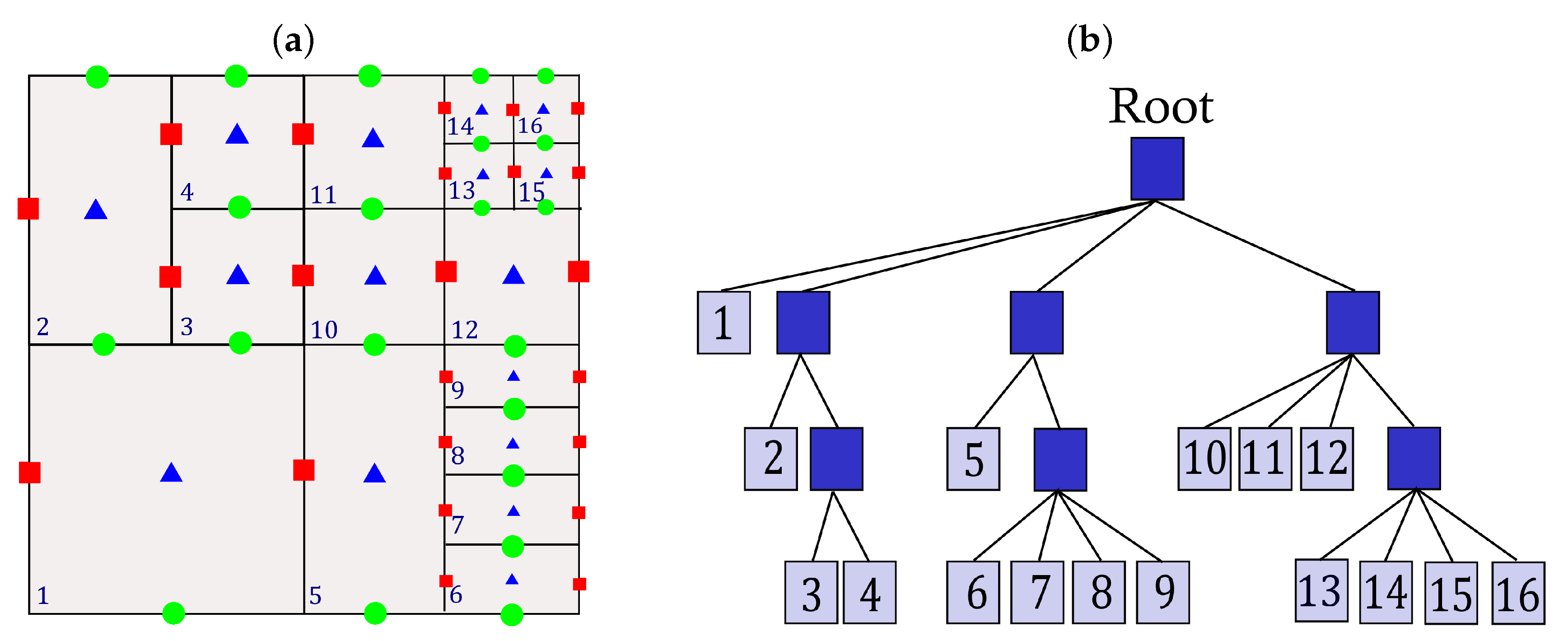
Figure 5 shows the non-uniform meshes, where we can see the structure of the mesh. In Figure 5a, the mesh $MRI$ (with two levels of refinement) is depicted, and in Figure 5b, we can see the mesh $MRVI$ (with three levels of refinement).

The u-profiles are illustrated in Figure 6, where the mesh convergence can be seen. We adopted mesh $MV$ as a reference mesh (black line) and the solutions of the refined meshes (full symbols) and uniform meshes (empty symbols) are shown. In this figure, we also show the OpenFoam system profile using the mesh MV. We saw good agreement between the solutions obtained in both systems.

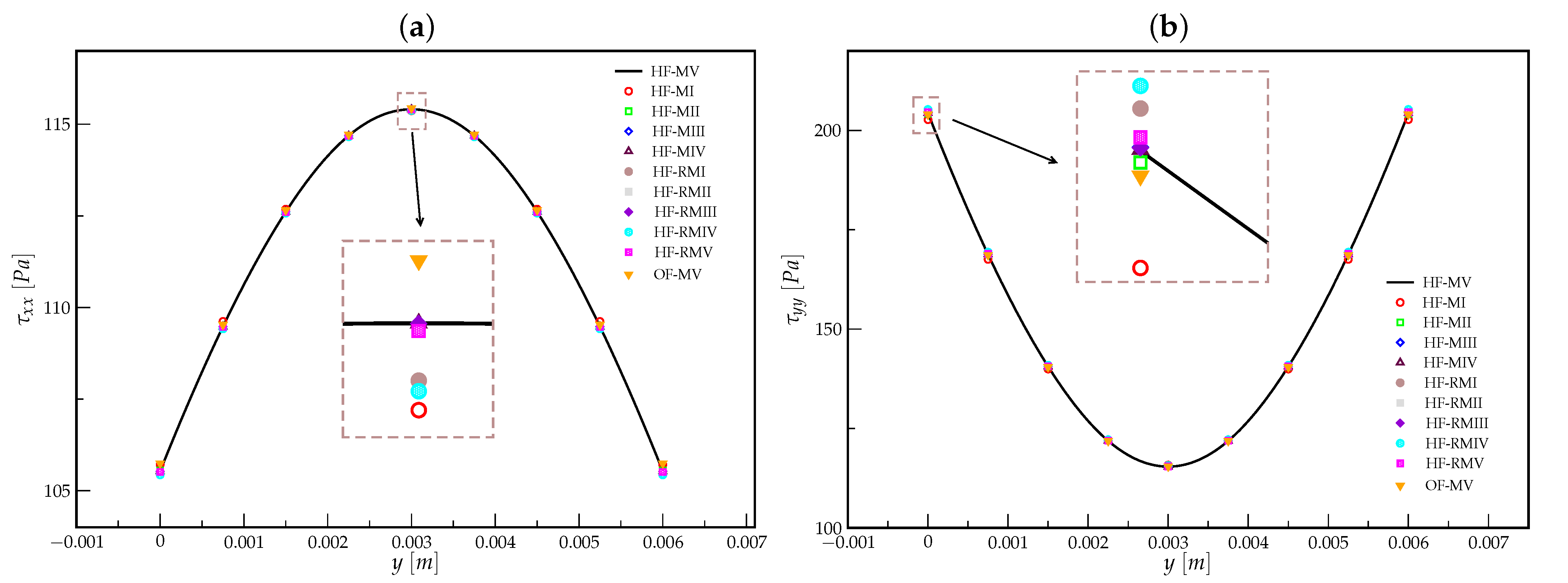
Our results for the tensor components ${\tau }_{xx}$ and ${\tau }_{yy}$ are presented in Figure 7, where we can also see good agreement between the numerical solutions of the HiGFlow and the OpenFOAM systems.

To verify the convergence, we show the errors ($L_1$, $L_2$, $L_{\infty }$) and the orders in

Table 5. Errors and orders for u-velocity. The mesh $MV$ was assumed as a reference solution.

${\mathit{u}}_{\mathit{x}}$ Errors
Mesh	${\mathit{L}}_{\mathbf{1}}$	${\mathit{L}}_{\mathbf{2}}$	${\mathit{L}}_{\infty }$
MI	$1.046\times {10}^{-3}$	$1.012\times {10}^{-3}$	$1.022\times {10}^{-3}$
MII	$1.718\times {10}^{-4}$	$1.815\times {10}^{-4}$	$2.327\times {10}^{-4}$
MIII	$3.602\times {10}^{-5}$	$3.657\times {10}^{-5}$	$4.493\times {10}^{-5}$
MIV	$5.619\times {10}^{-6}$	$5.897\times {10}^{-6}$	$7.583\times {10}^{-6}$
RMI	$4.809\times {10}^{-4}$	$5.598\times {10}^{-4}$	$7.115\times {10}^{-4}$
RMII	$1.007\times {10}^{-4}$	$1.018\times {10}^{-4}$	$1.110\times {10}^{-4}$
RMIII	$2.253\times {10}^{-5}$	$2.238\times {10}^{-5}$	$2.382\times {10}^{-5}$
RMVI	$5.306\times {10}^{-4}$	$5.452\times {10}^{-4}$	$5.918\times {10}^{-4}$
RMV	$1.077\times {10}^{-4}$	$1.129\times {10}^{-4}$	$1.250\times {10}^{-4}$
${\mathit{u}}_{\mathit{x}}$Orders
Mesh	${\mathit{L}}_{\mathbf{1}}$	${\mathit{L}}_{\mathbf{2}}$	${\mathit{L}}_{\infty }$
MI-MII	2.606	2.479	2.134
MII-MIII	2.254	2.311	2.373
MIII-MIV	2.680	2.633	2.567

. The errors are calculated using the following equations:

$$L_1=\frac{{\sum }_0^n\left|u{\left(i\right)}^{MV}-u{\left(i\right)}^{*}\right|}{{\sum }_0^n\left|u{\left(i\right)}^{*}\right|},L_2=\sqrt{\frac{{\sum }_0^n(u{\left(i\right)}^{MV}-u{\left(i\right)}^{*}{)}^2}{{\sum }_0^n{u{\left(i\right)}^{*}}^2}}\mathrm{and}{L}_{\infty }=\frac{max|u{\left(i\right)}^{MV}-u{\left(i\right)}^{*}|}{max|u{\left(i\right)}^{*}|}$$

where $u{\left(i\right)}^{MV}$ is the solution in mesh $MV$ and $u{\left(i\right)}^{*}$ is the solution in meshes $MI-MIV$ and $MRI-MRV$, $u\left(i\right)$ is the $u_x$ profile in points $i=\left(x\right(i),y(i\left)\right)$ in which $x\left(i\right)=5$ and $y\left(i\right)=i*0.125$, $i=0,1,\cdots ,8$. The orders Q for uniform meshes $Q=\frac{log\left(E_{M2}\backslash E_{M1}\right)}{log\left(h_2\backslash h_1\right)}$ show values close to 2 ($Q\approx 2$), which is the correct value that we expected to observe, since the velocity is calculated using an implicit Euler method. The values $E_{M2}$ and $E_{M1}$ are the errors (in the norms $L_1$, $L_2$ or $L_{\infty }$) for two consecutive meshes (the $d_x$ value in $M_2$ is lower than in $M_1$) and $h_2$ and $h_1$ are the $d_x$ values in their respective meshes.

4.2. Numerical Simulation of 4:1 Abrupt Planar Contraction Problem

In this section, we show the simulations for the 4:1 abrupt planar contraction flow. This problem is interesting because, for instance, the flow near the contraction is a complex mixture of shear and elongation, and secondary fluid motions might exist, even in the Newtonian limit (see [15]). For this reason, contraction flows have been extensively studied previously in the literature (see [3,14,15,26]).

Figure 8 shows the domain representation, where we adopted a dimensionless parabolic inlet velocity profile $u\left(y\right)=\frac{3}{8}\frac{1}{4}(2-y)(2+y)$. The scaling parameter $L=0.0064$ m is the height of the small channel, and we used $N=50$ deformation fields, $ϵ=0.1$ and the time interval $s_c=0.1$ s. In

Table 6. Flow parameter values used in the contraction problem.

Planar Contraction Flows
$\overline{\mathit{u}}\left[\frac{\mathit{m}}{\mathit{s}}\right]$	$\dot{\mathit{\gamma }}\left[\frac{\mathbf{1}}{\mathit{s}}\right]$	$\mathit{De}\left(\dot{\mathit{\gamma }}\right)$	$\mathit{Re}$	$\mathit{De}$
0.044	13.9	0.38	0.16	0.41
0.100	31.3	0.55	0.36	0.94
0.150	48.4	0.66	0.56	1.45
0.221	69.1	0.77	0.80	2.07

, we report the scaling parameters of average velocity $\overline{u}$ used in all simulations and the dimensionless parameters $Re=\frac{\rho LU}{{\eta }_0}$, $De=\frac{\lambda U}{L}$, $De\left(\dot{\gamma }\right)$ (see [15]) and the characteristic shear rate $\dot{\gamma }$.

The mesh $M_1$ used in these simulations is shown in Figure 9. We used three levels of refinement, with the most refined part near the contraction region. We also used one uniform mesh $M_2$ for $De=0.94$ in order to check the convergence solutions in two meshes. In $M_2$, $d_x=d_y=0.03125$ m, and in $M_1$, we use small values of $dx=dy=0.03125$ m as well as larger values, $dx=dy=0.125$ m.

In Figure 10, we illustrate the centerline axial profile velocity $u_x\left(y\right)$ solutions for different values of the Deborah number $De=0.41,0.94,1.45$ and $2.07$ for the HiGFlow (green lines) and OpenFOAM (black lines) systems using mesh $M1$. The experimental results of Quinzani et al. [15] and numerical results of Mitsoulis [14] and Tomé et al. [3] (for $De=1.45$) are also shown for comparison purposes. For the case with $De=0.94$, we show two solutions using our methodology in mesh $M_1$ (non-uniform mesh) and mesh $M_2$, where we can see good agreement between the solutions. For this reason, we adopted the $M_1$ mesh to simulate the other cases with different values of number $De$. For the profile $u_x\left(y\right)$, the HiGFlow system showed good agreement with the OpenFOAM solutions in the regions before and after the contraction. Near to contraction (see Figure 10), we have a region of instability and the methodology behaves differently, but our results showed similar behavior to the instabilities presented in the works of Quinzani et al. (orange triangles) [15], Mitsoulis [14] (blue bullet) and Tomé et al. (violet square) [3].

In Figure 11, we show the numerical solution using HiGFlow (green lines) and OpenFOAM (black lines) systems for the tensor components ${\tau }_{xx}$ and ${\tau }_{yy}$ with the same flow parameter values reported in Table 6 using $M_1$ and $M_2$ for the case with $De=0.94$. The methodologies presented in this work are different. OpenFOAM uses the finite volume method while HiGFlow approximates the equations using finite differences. Therefore, the solutions obtained will not be equal but should be comparable. Outside the contraction region, the OpenFOAM and HiGFlow solutions are very similar for all values of $De$. However, in the region close to the contraction, the solutions obtained using OpenFOAM showed a higher peak ($x\approx 0$) but this is mostly seen in the cases with the highest values of $De$.

In Figure 12a, we show the comparison between the first normal stress difference values $N1={\tau }_{xx}-{\tau }_{yy}$ for two different cases of Deborah number, $De=0.41$ and $De=1.45$. For better visualization, the other two values of $De$ (see Table 6) are illustrated in Figure 12b, where we can see that the values of HiGFlow (green lines) have good agreement with experimental data (orange triangles) reported by Quinzani [15], while the solution using OpenFOAM was similar to the solution presented by Mitsoulis [14].

In Figure 13, we compare the streamlines obtained using OpenFOAM (a) and HiGFlow (b) with a fixed value of $De=2.07$. We can see that there is vortex formation in both cases and that the solutions are relatively comparable.

5. Discussion

The work aims to present the numerical simulation of the KBKZ integral constitutive equations for incompressible and transient complex flows. We used a new solver HiGTree/HiGFlow lately developed by Souza et al. [23]. In this solver, we have implemented the methodology described in Section 3.1 to simulate viscoelastic flows modeled by integral constitutive equations. Initially, the numerical technique was verified by refined mesh in channel flows. Using the FLUID $S1$ (see Table 2), we performed nine simulations using non-refined and refined meshes. For comparison purposes, a mesh was chosen and the simulation using the OpenFOAM solver [26] was performed. In these simulations, we can see that, although the methodologies used in HiGFlow and OpenFOAM are quite different (the first uses finite differences and the second uses finite volume), we obtained very similar results in both systems. We also verified that the errors decrease with the mesh refinement and that the order of convergence of the velocity was around two, as expected.

A classic problem in the simulation of integral viscoelastic flows is known as 4:1 abrupt contraction and, thus, the literature for this problem is extensive. We chose to check our methodology for the four values of $De$ presented in Mitsoulis [14]. In addition to the comparison with the results of this author, we performed the simulations using the OpenFOAM solver [26] and also compared our results with the experimental ones from Quinzani [15] and with the numerical results from FreeFlow [3]. We know that, in the contraction region, there are singularities and numerical techniques that might exhibit different behaviors. Although the values obtained by us in this work differ somewhat from the values obtained by Mitsoulis [14] or OpenFOAM [26], they were quite comparable to the experimental values of Quinzani [15]. Thus, we verified that the methodology presented here is capable of simulating complex flows in transient fluid regimes governed by integral constitutive models using the rapid technique of finite differences in hierarchical meshes with local refinement.

The computational efficiency of the models has been previously studied [3,21,26]. However, it is worth mentioning that the methods used in the present work used fewer integration points (deformation fields) compared to the points used in the early work of Hulsen et al. [28] and are similar to those used more recently by Hulsen and Anderson [32]. This improvement is due mainly to the distinct methodologies adopted to obtain the integration points, which allow efficient distribution of the elapsed time. Although the results presented here are two-dimensional, our methodology is still able to simulate flows in higher dimensions (the user just has to specify the dimension (2, 3 or higher) in the input data file). Our future work will be to present simulations in three dimensions for classic problems. In three dimensions, for example, integral models are still computationally expensive, as there is a need to store and connect a fixed N number of fields to each cell. Therefore, we will also work on ways to improve or modify the integral calculation—for instance, as was done in the recent work of Hulsen [32].

References

1. Aboubacar, M.; Matallah, H.; Tamaddon-Jahromi, H.R.; Webster, M.F. Highly elastic solutions for Oldroyd-B and Phan-Thien Tanner fluids with a finite volume element method: Planar contraction flows. J. Non-Newt. Fluid Mech. 2020, 103, 65–103. [Google Scholar] [CrossRef]
2. Clermont, J.R.; Normandin, M. Numerical simulation of extrudate swell for Oldroyd-B fluid using the stream-tube analysis and a streamline approximation. J. Non-Newt. Fluid Mech. 1993, 50, 193–215. [Google Scholar] [CrossRef]
3. Tomé, M.F.; Araujo, M.S.B.; Alves, M.A.; Pinho, F.T. Numerical simulation of viscoelastic flows using integral constitutive equations: A finite difference approach. J. Comput. Phys. 2008, 227, 4207–4243. [Google Scholar] [CrossRef]
4. Tomé, M.F.; Castelo, A.; Afonso, A.M.; Alves, M.A.; Pinho, F.T. Application of the log-conformation tensor to three-dimensional time-dependent free surface flows. J. Non-Newt. Fluid Mech. 2012, 175–176, 44–54. [Google Scholar] [CrossRef]
5. Mompean, G.; Thais, L.; Tomé, M.F.; Castelo, A. Numerical prediction of three-dimensional time-dependent viscoelastic extrudate swell using differential and algebraic models. Comput. Fluids 2011, 44, 68–78. [Google Scholar] [CrossRef]
6. Berauto, C.; Fortin, A.; Coupez, T.; Demay, Y.; Vergnes, B.; Agassant, J.F. A finite element method for computing the flow of multi-mode viscoelastic fluids: Comparison with experiments. J. Non-Newt. Fluid Mech. 1998, 75, 1–23. [Google Scholar] [CrossRef]
7. Tomé, M.F.; Paulo, G.S.; Alves, M.A.; Pinho, F.T. Numerical Solution of the PTT constitutive equation for three-dimensional free surface flows. J. Non-Newt. Fluid Mech. 2010, 165, 247–262. [Google Scholar] [CrossRef]
8. Oishi, C.M.; Martins, F.P.; Tomé, M.F.; Alves, M.A. Numerical simulation of drop impact and jet buckling problems using the eXtended Pom Pom model. J. Non-Newt. Fluid Mech. 2012, 169–170, 91–103. [Google Scholar] [CrossRef]
9. Oishi, C.M.; Martins, F.P.; Tomé, M.F.; Cuminato, J.A.; Mckee, S. Numerical solution of the eXtended Pom-Pom model for viscoelastic free surface flows. J. Non-Newt. Fluid Mech. 2011, 166, 165–179. [Google Scholar] [CrossRef] [Green Version]
10. Tanner, R.I. From A to (BK)Z in constitutive relations. J. Rheol. 1988, 32, 673–702. [Google Scholar] [CrossRef]
11. Mitsoulis, E. 50 Years of the K-BKZ constitutive relation for polymers. Polym. Sci. 2013. [Google Scholar] [CrossRef]
12. Luo, X.L.; Mitsoulis, E. An efficient algorithm for strain history tracking in finite element computation of non-Newtonian fluids with integral constitutive equations. Int. J. Num. Meth. Fluids 1990, 11, 1015–1031. [Google Scholar] [CrossRef]
13. Ansari, M.; Alabbas, A.; Hatzikiriakos, S.G.; Mitsoulis, E. Entry flow of polyethylene melts in tapered dies. Int. Polym. Proc. 2010, 25, 287–296. [Google Scholar] [CrossRef]
14. Mitsoulis, E. Numerical simulation of planar entry flow for a polyisobutylene solution using an integral constitutive equation. J. Rheol. 1993, 37, 1029. [Google Scholar] [CrossRef]
15. Quinzani, L.M.; Brown, R.A.; Armstrong, R.C. Birefringence and laser-Doppler velocimetry (LDV) studies of viscoelastic flow through a planar contraction. J. Non-Newt. Fluid Mech. 1994, 52, 1–36. [Google Scholar] [CrossRef]
16. McKinley, G.H.; Sridhar, T. Filament-stretching rheometry of complex fluids. Annu. Rev. Fluid Mech. 2002, 34, 375–415. [Google Scholar] [CrossRef] [Green Version]
17. Chai, M.S.; Yeow, Y.L. Modelling of fluid M1 using multiple-relaxation-time constitutive equations. J. Non-Newt. Fluid Mech. 1990, 35, 459–470. [Google Scholar] [CrossRef]
18. Mitsoulis, E. Extrudate swell of Boger fluids. J. Non-Newt. Fluid Mech. 2010, 165, 812–824. [Google Scholar] [CrossRef]
19. Ganvir, V.; Lele, A.; Thaokar, R.; Gautham, B.P. Prediction of extrudate swell in polymer melt extrusion using an arbitrary Langrangian Eulerian (ALE) based finite element method. J. Non-Newt. Fluid Mech. 2009, 156, 21–28. [Google Scholar] [CrossRef]
20. Ahmed, R.; Liang, R.F.; Mackley, M.R. The experimental observation and numerical prediction of planar entry flow and die swell for molten polyethylenes. J. Non-Newt. Fluid Mech. 1995, 59, 129–153. [Google Scholar] [CrossRef]
21. Tomé, M.F.; Bertoco, J.; Oishi, C.M.; Araujo, M.S.B.; Cruz, D.; Pinho, F.T.; Vynnycky, M. A finite difference technique for solving a time strain separable k-bkz constitutive equation for two-dimensional moving free surface flows. J. Comput. Phys. 2016, 311, 114–141. [Google Scholar] [CrossRef] [Green Version]
22. Losasso, F.; Gibou, F.; Fedkiw, R. Simulating water and smoke with an octree data structure. ACM Trans. Grap. (TOG) 2004, 3, 457–462. [Google Scholar] [CrossRef]
23. Sousa, F.S.; Lages, C.F.; Ansoni, J.L.; Castelo, A.; Simão, A. A finite difference method with meshless interpolation for incompressible flows in non-graded tree-based grids. J. Comput. Phys. 2019, 396, 848–866. [Google Scholar] [CrossRef]
24. Weller, H.G.; Tabor, G.; Jasak, H.; Fureby, C. A tensorial approach to computational continuum mechanics using object-oriented techniques. Comp. Phys. 1998, 12, 620–631. [Google Scholar] [CrossRef]
25. Papanastasiou, A.C.; Scriven, L.E.; Macosko, C.W. An integral constitutive equation for mixed flows: Viscoelastic characterization. J. Rheol. 1993, 27, 387. [Google Scholar] [CrossRef]
26. Araújo, M.S.B.; Fernandes, C.; Ferrás, L.L.; Tukovic, Z.; Jasakc, H.; Nóbrega, J.M. A stable numerical implementation of integral viscoelastic models in the OpenFOAM computational library. Comput. Fluids 2018, 172, 1–13. [Google Scholar] [CrossRef]
27. Chorin, A.J. Numerical solution of the Navier-Stokes equations. Math. Comp. 1968, 22, 745–762. [Google Scholar] [CrossRef]
28. Hulsen, M.A.; Peters, E.; Brule, B.V.D. A new approach to the deformation fields method for solving complex flows using integral constitutive equations. J. Non-Newt. Fluid Mech. 2001, 98, 201–221. [Google Scholar] [CrossRef]
29. Alves, M.; Oliveira, P.; Pinho, F.T. A convergent and universally bounded interpolation scheme for the treatment of advection. Int. J. Num. Meth. Fluids 2003, 41, 47–75. [Google Scholar] [CrossRef]
30. Fernandes, C.; Araujo, M.S.B.; Ferrás, L.L.; Nóbrega, J.M. Improved both sides diffusion (iBSD): A new and straightforward stabilization approach for viscoelastic fluid flows. J. Non-Newt. Fluid Mech. 2017, 49, 63–78. [Google Scholar] [CrossRef] [Green Version]
31. Van der Vorst, H.A. Bi-CGSTAB: A Fast and Smoothly Converging Variant of Bi-CG for the Solution of Nonsymmetric Linear Systems. SIAM J. Sci. Stat. Comput. 1992, 13, 631–644. [Google Scholar] [CrossRef]
32. Hulsen, M.A.; Anderson, P.D. The deformation fields method revisited: Stable simulation of instationary viscoelastic fluid flow using integral models. J. Non-Newt. Fluid Mech. 2018, 262, 68–78. [Google Scholar] [CrossRef]
Figure 1. HiGTree data structure: (a) computational cell representation, (b) tree-based data structures.
Applsci 11 04875 g001
Figure 2. Finite difference 2nd-order stencil discretization.
Applsci 11 04875 g002
Figure 3. Computational domain used in OpenFOAM for the contraction problem.
Applsci 11 04875 g003
Figure 4. Dimensionless representation of the channel domain.
Applsci 11 04875 g004
Figure 5. Refined meshes: (a) two levels and (b) three levels.
Applsci 11 04875 g005
Figure 6. The u-profiles used by simulation of channel problem.
Applsci 11 04875 g006
Figure 7. Comparison between the sumerical solutions of the tensor components obtained using HiGFlow (with different meshes) and OpenFOAM (mesh M V ). (a) τ x x and (b) τ y y tensor components.
Applsci 11 04875 g007
Figure 8. Domain representation.
Applsci 11 04875 g008
Figure 9. Graphical representation of the mesh M 1 used in the contraction simulation.
Applsci 11 04875 g009
Figure 10. Centerline axial velocity profiles obtained using HiGFlow (green lines) and OpenFOAM (black lines). Experimental [15] and numerical results [3,14] found in the literature are also shown for comparison purposes.
Applsci 11 04875 g010
Figure 11. Numerical results for (a) τ x x and (b) τ y y using HiGFlow system (HF-M1 e HF-M2) and OpenFOAM system (OF-M1).
Applsci 11 04875 g011
Figure 12. The first normal stress differences N 1 : (a) for D e = 0.41 and D e = 1.45 ; and (b) for D e = 0.94 and D e = 2.07 .
Applsci 11 04875 g012
Figure 13. Streamlines of the contraction flow problem with D e = 2.07 . (a) OpenFOAM and (b) HiGFlow.
Applsci 11 04875 g013