A Backwards-Tracking Lagrangian-Eulerian Method for Viscoelastic Two-Fluid Flows

Abstract

A new Lagrangian–Eulerian method for the simulation of viscoelastic free surface flow is proposed. The approach is developed from a method in which the constitutive equation for viscoelastic stress is solved at Lagrangian nodes, which are convected by the flow, and interpolated to the Eulerian grid with radial basis functions. In the new method, a backwards-tracking methodology is employed, allowing for fixed locations for the Lagrangian nodes to be chosen a priori. The proposed method is also extended to the simulation of viscoelastic free surface flow with the volume of fluid method. No unstructured interpolation or node redistribution is required with the new approach. Furthermore, the total amount of Lagrangian nodes is significantly reduced when compared to the original Lagrangian–Eulerian method. Consequently, the method is more computationally efficient and robust. No additional stabilization technique, such as both-sides diffusion or reformulation of the constitutive equation, is necessary. A validation is performed with the analytic solution for transient and steady planar Poiseuille flow, with excellent results. Furthermore, the proposed method agrees well with numerical data from the literature for the viscoelastic die swell flow of an Oldroyd-B model. The capabilities to simulate viscoelastic free surface flow are also demonstrated through the simulation of a jet buckling case.

1. Introduction

Viscoelastic free surface flows are of significant importance for many industrial processes. This includes polymer extrusion, additive manufacturing, seam sealing, and adhesive joining. In such processes, the viscoelastic properties of the flow, such as the flow history, can have major influence on the quality of the final product. Furthermore, production time and raw materials may be subject to a large cost. Therefore, extensive manual effort and physical testing may be necessary to optimize the process in terms of product quality, material consumption, and production cycle time.

Numerical tools can be helpful in reducing the manual preparation time, as they offer the possibility to replace a significant part of the physical testing with computer simulation. Furthermore, numerical simulations may enable testing early in the design phase. For many complex industrial applications, a large demand for suitable numerical simulation tools therefore exists. Furthermore, for such tools to be useful, high demands are put on accuracy, robustness, and computational efficiency.

A common approach for simulating viscoelastic fluid flow is to discretize the governing equations in the Eulerian frame of reference with the finite volume method (FVM) [1,2,3] or the finite element method (FEM) [4,5]. The Eulerian frame of reference is suitable for diffusion-dominated problems, including viscous fluid flow as well as heat and mass transfer. On the other hand, viscoelastic constitutive equations are typically hyperbolic and they involve no physical diffusion term. Thus, in this sense, the Lagrangian frame of reference is a more natural description for the constitutive equation. Therefore, Lagrangian or semi-Lagrangian methods are appealing as alternative approaches to the Eulerian frame.

Rasmussen and Hassager [6] developed a Lagrangian finite element method in order to calculate the flow of an upper convected Maxwell (UCM) fluid. The entire flow history was stored and re-meshing was required, due to deformation. Harlen et al. [7] proposed a split Lagrangian–Eulerian method for viscoelastic Stokes flow. The constitutive equation was solved at the nodes of a co-deforming mesh, while the momentum and continuity equations were solved with an Eulerian finite element method. Re-meshing due to mesh distortion was also used in their method. Halin et al. proposed the Lagrangian particle method (LPM) [8]. In their method, the momentum and continuity equations were solved with the Eulerian finite element method. The constitutive equation was solved along the trajectories of massless Lagrangian particles. The stresses in the particles were then fitted to local polynomial expressions in order to enable the evaluation of the corresponding finite element integrals in the momentum. Hence, a minimum of three particles per two-dimensional element was required for the polynomial approximations to be feasible. Later on, the adaptive Lagrangian particle method (ALPM) [9] was proposed, utilizing adaptive addition and the deletion of particles. However, a fairly large number of particles was required for the simulations to produce stable transient results. Furthermore, Wapperom et al. [10] proposed the backward-tracking Lagrangian particle method (BLPM), in which backwards integration of the velocity field allowed for the choice of fixed particle locations a priori, increasing the efficiency of their particle tracking approach.

The simulation of viscoelastic free surface flow has been approached with different methods. For example, Crochet and Keunings [11] simulated the viscoelastic die swell effect of an Oldroyd-B fluid with a mixed finite element method as early as 1982. More recent similar examples of finite element methods on non-stationary grids can be found in Balemans et al. [12] and Spanjaards et al. [13]. The marker-and-cell (MAC) approach is a method that has been used quite extensively for simulation free surface flows [14,15,16,17,18,19,20], in which the governing equations discretized with finite differences and the free surface is tracked while using marker particles. The method has been successfully used for the simulation, for example, of the die swell and viscoelastic jet buckling with a variety of constitutive models. The simulations are typically performed on staggered, uniform grids, which has certain limitations for complex simulation geometries and in terms of computational efficiency when high resolution is required. Furthermore, the existence of a gas phase surrounding the viscoelastic fluid is not taken into account, which may be required for some cases. The front-tracking method is another similar method [21].

The volume of fluid (VOF) method is a popular method for the simulation of Newtonian as well as viscoelastic free surface flow with finite volume discretization. VOF is a diffuse–interface method, in which the presence of two or more fluid phases is represented by their corresponding volume fractions, advected with geometric or algebraic schemes. A sharp fluid interface may then be reconstructed from the solution. A single set of momentum, continuity equations are then solved for the whole domain, and the fluid properties are locally averaged with the fluid volume fraction. Furthermore, the transport of the volume fraction may be solved with the same spatial grid as the momentum and continuity equation, which makes the method suitable for finite volume simulation of free surface flow. Some examples follow.

Habla et al. [22] developed a VOF-solver for viscoelastic free surface flow that is based on the open source solver OpenFOAM [23]. The simulations were stabilized by reformulating the viscoelastic constitutive equations with the log-conformation representation (LCR) and with both-sides diffusion (BSD) in the momentum equation. Comminal et al. [24] simulated the viscoelastic die swell effect for Oldroyd-B and Giesekus fluids with the VOF method, combined with two different schemes for the convection of the fluid volume fraction, a geometric scheme, as well as an algebraic scheme that directly solved the transport equation for the volume fraction. Furthermore, their methods were compared to the VOF solver that is available in RheoTool [25], which is an open source toolbox for viscoelastic flow that is based on OpenFOAM. The constitutive equation was also reformulated with LCR in their study. Bonito et al. [26] reported a related method, using a mathematical formulation that is similar to the volume of fluid method, while solving the governing equations with a piecewise linear finite element method, contrary to finite volume discretization.

In previous work, a Lagrangian–Eulerian framework for viscoelastic flow has been proposed [27,28]. In the method, the constitutive equation is solved at Lagrangian nodes, which are convected by the flow. The momentum and continuity equations are discretized with the finite volume method on an Eulerian octree grid and then solved with SIMPLEC iterations [29]. Boundary conditions that are imposed by objects in the domain are treated using implicit immersed boundary methods [30,31]. The contribution to the momentum equation from the viscoelastic stress is established through the unstructured interpolation of the stress tensors from the Lagrangian nodes to the cell centers of the Eulerian grid while using the radial basis function.

The ability to efficiently simulate industrial applications, such as adhesive extrusion, parts assembly, and additive manufacturing, is a main motivator to develop the new method. For this purpose, it is necessary that the numerical method is accurate, computationally efficient, and robust. The ability to model viscoelastic free surface flow in complex geometry with moving objects is also necessary. The proposed method was shown to produce results in good agreement with available analytic and numerical data from the literature [27]. It has also been shown that the Lagrangian formulation of the constitutive equation allows for the efficient parallelization of the viscoelastic stress calculation, which makes the method highly suitable for GPU-acceleration [28]. Furthermore, the use of an immersed boundary method in combination with the automatically generated grid enables simulation on arbitrary geometry with minimal pre-processing.

In the previous studies [27,28], the proposed Lagrangian–Eulerian method has been validated for single-phase flows with uniform grids. The natural next steps include enabling the simulation of free surface flow as well as simulation on refined grids. Therefore, in the current work, the proposed method is further developed in these two aspects. Firstly, the framework is extended for simulation of viscoelastic free surface flows with the volume of fluid method. Secondly, a backwards-tracking procedure is introduced to the solution of the constitutive equation, partly inspired by the backward-tracking Lagrangian particle method by Wapperom et al. [10]. The result is a more robust method, due to the structured relation between the Lagrangian nodes and the Eulerian grid. No stabilization method, i.e., neither both-sides diffusion nor reformulation of the constitutive equation, is required for the studied flows. Furthermore, the computational cost as compared to the original Lagrangian–Eulerian method is reduced, since no unstructured interpolation or node redistribution is needed and because the total number of Lagrangian nodes decreased. In the context of multiphase flows, the viscoelastic constitutive equation is only solved inside the viscoelastic phase, which further increases the computational performance.

The rest of the paper is structured, as follows. In the next section, the governing equations are presented, followed by a detailed description of the proposed numerical method. In the results section, the new method demonstrated and validated with analytic solutions and numerical data from the literature. Finally, conclusions are drawn and future work is outlined.

2. Governing Equations

Viscoelastic fluid flow is described by the incompressible momentum and continuity equations

$$\rho \left(\frac{\partial \mathbf{u}}{\partial t}+\mathbf{u}·\nabla \mathbf{u}\right)=-\nabla p+\nabla ·(2\mu \mathbf{S}+\mathit{\tau })+\mathbf{f},$$

(1)

$$\nabla ·\mathbf{u}=0,$$

(2)

where $\rho$ is the density, $\mathbf{u}$ velocity, $\mu$ the solvent viscosity, $\mathbf{S}=\frac{1}{2}(\nabla \mathbf{u}+{(\nabla \mathbf{u})}^T)$ the strain rate tensor, $\mathit{\tau }$ the viscoelastic stress tensor, and $\mathbf{f}$ a body force. The viscoelastic stress is governed by a constitutive equation of the general form

$$\lambda \stackrel{▽}{\mathit{\tau }}+F\left(\mathit{\tau }\right)\mathit{\tau }=2\eta \mathbf{S},$$

(3)

where $\lambda$ is the relaxation time, $\eta$ polymeric viscosity, and F a scalar-valued function. The operator $\stackrel{▽}{(•)}$ denotes the upper-convected derivative of $\mathit{\tau }$, which expands to

$$\stackrel{▽}{\mathit{\tau }}=\frac{D\mathit{\tau }}{Dt}-{(\nabla \mathbf{u})}^T·\mathit{\tau }-\mathit{\tau }·\nabla \mathbf{u},$$

(4)

where

$$\frac{D\mathit{\tau }}{Dt}=\frac{\partial \mathit{\tau }}{\partial t}+\mathbf{u}·\nabla \mathit{\tau },$$

(5)

is the Lagrangian, or material, time derivative of $\mathit{\tau }$. The Lagrangian time derivative describes the rate of change of $\mathit{\tau }$ in an infinitesimal material element, which moves with the flow. Convected time derivatives, such as $\stackrel{▽}{(•)}$, appear in viscoelastic constitutive equations and they ensure frame-invariance for the transport of tensorial properties. It is remarked that, while the form of (3) is not applicable for all available differential constitutive equations, it covers the constitutive models discussed in this work.

In general, the viscoelastic stress tensor may be modeled as a sum of the contribution of N modes as

$$\mathit{\tau }=\sum _{k=1}^N{\mathit{\tau }}_k,$$

(6)

where ${\mathit{\tau }}_k$ is the stress tensor that corresponds to the kth mode. Each stress tensor ${\mathit{\tau }}_k$ is then governed by a constitutive equation on the form of (3) with an individual set of model parameters.

3. Numerical Method

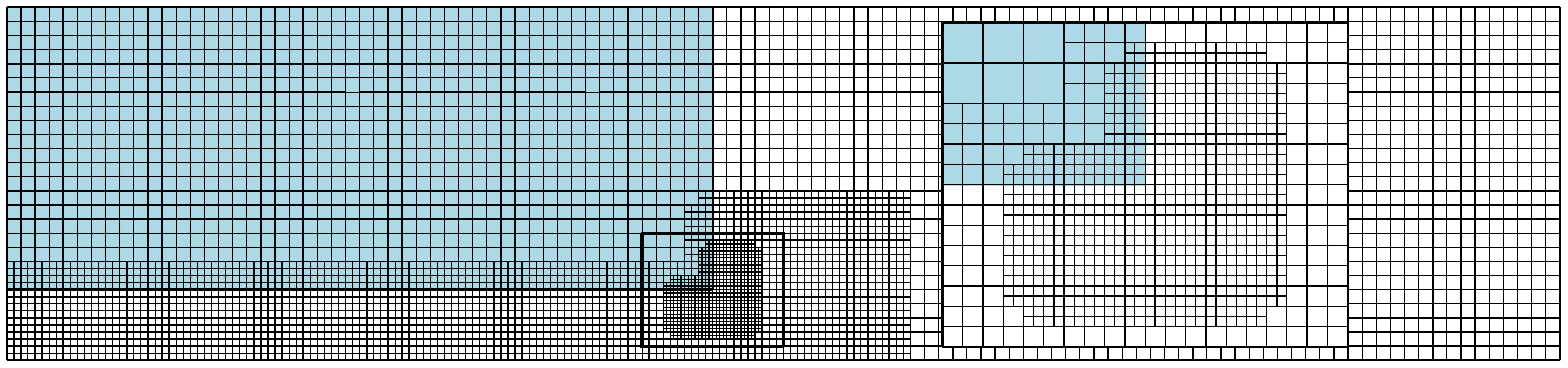
The momentum Equation (1) and the continuity Equation (2) are discretized on a collocated Eulerian grid with the finite volume method. The pressure–velocity coupling is accomplished by solving the momentum and continuity equations with SIMPLEC iterations [32]. An octree grid is used, in which the cells can be refined in desired locations by recursively dividing them into smaller cells to a given refinement level. The refinements may be static or adaptively updated, typically around moving objects or fluid interfaces. Figure 1 displays an example grid in two dimensions with one refinement level, showing the cell centers and the grid nodes. The grid, including the adaptive refinements, is automatically generated by the solver.

Boundary conditions from objects in the domain are imposed while using the mirroring immersed boundary method [30,31]. The velocity field is implicitly mirrored across the immersed boundary surface, such that the imposed boundary condition is satisfied for the converged solution. Surface triangulations represent the geometrical objects.

The viscoelastic constitutive equation is solved in the Lagrangian frame of reference in material elements that are represented as Lagrangian nodes. From (3) and (4), it follows that the stress in a Lagrangian node is described by the ordinary differential equation (ODE)

$$\frac{D\mathit{\tau }}{Dt}=\frac{2\eta }{\lambda }\mathbf{S}-\frac{1}{\lambda }F\left(\mathit{\tau }\right)\mathit{\tau }+{(\nabla \mathbf{u})}^T·\mathit{\tau }+\mathit{\tau }·\nabla \mathbf{u}.$$

(7)

Furthermore, the trajectory of the node must be known when solving (7), as it involves the local velocity gradient $\nabla \mathbf{u}$. The trajectory of the node is given by the ODE

$$\frac{D\mathbf{x}}{Dt}=\mathbf{u},$$

(8)

where $\mathbf{x}$ is the position of the node.

Given an initial stress state in a set of Lagrangian nodes, a straightforward approach to obtain the stress state at a future time is to simultaneously solve (7) and (8) forwards in time. Indeed, this method has been successfully employed in previous work [27,28]. Lagrangian nodes were then initialized with a given distribution density at the start of the simulation. The distribution was maintained in each time step by adding or deleting nodes, if necessary. After solving the constitutive equation at the Lagrangian nodes, the viscoelastic stress was interpolated to the Eulerian cell centers while using radial basis functions (RBF).

In this work, the method is further developed by introducing the concept of backwards-tracking. The key idea is to choose the locations of the Lagrangian nodes a priori, at which the viscoelastic stresses are then stored, and then track them backwards in time in order to obtain their initial location in each time step. The constitutive equation may then be solved forwards in time such that the stresses are obtained at for the next time step at the chosen locations. Different choices for the locations are conceivable. In the current work, the locations of the Lagrangian nodes are chosen to be at the Eulerian grid nodes.

Consider the calculation of the viscoelastic stress for the nth simulation step, which corresponds to the time interval $I_n=[t_n,t_{n+1}]$. At this point, it is assumed that momentum equation has been solved, such that the velocity field is known for $t\in I_n$.

The Lagrangian constitutive equation is solved along the trajectories of Lagrangian nodes. For a Lagrangian node, the trajectory $\mathbf{x}\left(t\right)$ can be expressed in terms of the position at the end of the time step, as

$$\mathbf{x}\left(t\right)=\mathbf{x}\left(t_{n+1}\right)-{\int }_t^{t_{n+1}}\mathbf{u}(t^{\prime },\mathbf{x}\left(t^{\prime }\right))d{t}^{\prime },t\in I_n,$$

(9)

where $\mathbf{x}\left(t_{n+1}\right)$ is the predefined final location of the Lagrangian node which. The trajectory $\mathbf{x}\left(t\right)$ for $t\in I_n$ is first calculated by solving (8) backwards in time. Subsequently, when the trajectory is known, the viscoelastic stress $\mathit{\tau }(t_n,\mathbf{x}\left(t_n\right))$ is interpolated from the viscoelastic stresses from the solution of the previous simulation step. The Lagrangian constitutive Equation (7) is then solved forwards in time and the viscoelastic stress is thus obtained at the final location $\mathbf{x}\left(t_n\right)$, i.e., at the predefined location.

Generally, the choice of locations for the Lagrangian nodes is somewhat arbitrary. However, by choosing the locations of the Eulerian grid nodes, the connectivity and structure of the octree grid may be utilized when the stress at time $t_n$ is interpolated to the position of a Lagrangian node $\mathbf{x}\left(t_n\right)$. The stress at the node at time $t_n$ is obtained through bilinear or trilinear interpolation, respectively, for two-dimensional (2D) and three-dimensiona (3D). Furthermore, the viscoelastic stress contribution to the discretized momentum equation may be calculated directly from node stresses. Therefore, no unstructured interpolation of viscoelastic stresses is necessary. The calculation of this contribution is described in detail further on in this section.

Figure 2 shows a schematic description of the steps that are involved in the algorithm. In summary, the performed steps are:

(a)

Calculate the Lagrangian node trajectory by solving (8) backwards in time, starting at the predefined location $\mathbf{x}\left(t_{n+1}\right)$.

(b)

Interpolate the stress $\mathit{\tau }(t_n,\mathbf{x}\left(t_n\right))$ to the Lagrangian node from the known node values at time $t_n$.

(c)

Solve (7) forwards in time along the trajectory $\mathbf{x}\left(t\right)$, $t\in I_n$.

The ordinary differential Equations (7) and (8) may be solved with any appropriate choice of ODE solution algorithm. In this work, the fourth order Runge–Kutta method, which is commonly referred to as the RK4 method [33], is used. Furthermore, $N_{\mathrm{sub}}$ equally sized substeps of length $\Delta t_{\mathrm{sub}}$ are used, being defined, such that $N_{\mathrm{sub}}\Delta t_{\mathrm{sub}}=\Delta t=t_{n+1}-t_n$. In the current work, $N_{\mathrm{sub}}=3$ is used.

When solving (7) and (8), local quantities that are stored on the Eulerian grid are required along the trajectory of the Lagrangian nodes. More specifically, the velocity $\mathbf{u}$ is needed for the backwards-tracking and the velocity gradient $\nabla \mathbf{u}$ is needed to solve the constitutive equation. The velocities are stored at the Eulerian cell centers. When the local velocity is required, the cell centers containing the Lagrangian node are identified and the velocity is interpolated to its location while using bilinear or trilinear interpolation, respectively, for 2D and 3D. When the velocity gradient is required, it is calculated from the bilinear or trilinear interpolation formula using the same interpolation basis.

For the interpolation of a field $\varphi$ to a location within a box spanned by the corners $(x_i,y_j,z_k)$, $i,j,k\in \{0,1\}$, the trilinear interpolation formula in order to calculate the interpolant $\widehat{\varphi }$ reads

$$\widehat{\varphi }=\sum _{i=0}^1\sum _{j=0}^1\sum _{k=0}^1{c}_x^i{c}_y^j{c}_z^k{\varphi }_{ijk},$$

(10)

where ${\varphi }_{ijk}$ is the value of $\varphi$ at the corner $(x_i,y_j,z_k)$ and with the coefficients

$$c_l^i=\left\{\begin{array}{cc}1-{\overline{x}}_l/\Delta x_l,& i=0\\ {\overline{x}}_l/\Delta x_l,& i=1\end{array}\right.,l=x,y,z,$$

(11)

where ${\overline{x}}_l$ is the lth coordinate of the interpolation position relative to the lower corner of the box and $\Delta x_l$ is the size of the box that coordinate direction. The gradient of $\widehat{\varphi }$ follows from (10) and (11), as

$$\frac{\partial \widehat{\varphi }}{\partial x}=\sum _{i=0}^1\sum _{j=0}^1\sum _{k=0}^1\left(\frac{\partial c_x^i}{\partial x}\right)c_y^j{c}_z^k{\varphi }_{ijk},$$

(12)

$$\frac{\partial \widehat{\varphi }}{\partial y}=\sum _{i=0}^1\sum _{j=0}^1\sum _{k=0}^1{c}_x^i\left(\frac{\partial c_y^j}{\partial y}\right)c_z^k{\varphi }_{ijk},$$

(13)

$$\frac{\partial \widehat{\varphi }}{\partial z}=\sum _{i=0}^1\sum _{j=0}^1\sum _{k=0}^1{c}_x^i{c}_y^j\left(\frac{\partial c_z^k}{\partial z}\right){\varphi }_{ijk},$$

(14)

where the derivatives of the coefficients read

$$\frac{\partial c_l^i}{\partial x_l}=\mp \frac{1}{\Delta x_l},i=0,1,l=x,y,z.$$

(15)

The corresponding formulas for bilinear interpolation in two dimensions are obtained by letting the coefficient $c_z^k=1$ and, thus, $\partial c_z^k/\partial z=0$, and skipping the summation over k.

When interpolating to a Lagrangian node near fluid grid refinements the smallest local cell size is used in order to form the interpolation box. Furthermore, not all corners of the interpolation box coincide with a cell center. The velocities at such corners are obtained through least squares interpolation, by fitting a first order polynomial from the centers of the cells that intersect the interpolation box. The interpolation box is visualized in Figure 3.

The volume of fluid (VOF) method is used to model the presence of a viscoelastic fluid phase and a Newtonian phase. A color function $\xi$, is then defined, such that

$$\xi =\left\{\begin{array}{c}1\mathrm{In}\mathrm{the}\mathrm{viscoelastic}\mathrm{phase}\\ 0\mathrm{In}\mathrm{the}\mathrm{Newtonian}\mathrm{phase}\end{array}\right\}.$$

(16)

The discrete counterpart of $\xi$ is the fluid volume fraction $\alpha \in [0,1]$, which is the local volume average of $\xi$ in an Eulerian cell. The transport of $\alpha$ is described by the convection equation [34]

$$\frac{\partial \alpha }{\partial t}+\mathbf{u}·\nabla \alpha =0.$$

(17)

By definition, $\alpha$ is the local volume fraction of the viscoelastic phase in a control volume. Hence, if $\alpha =1$, the control volume is filled with the viscoelastic fluid and if $\alpha =0$ with the Newtonian fluid. If $\alpha \in (0,1)$, this is interpreted as that the control volume intersects the interface between the fluid phases. The transport Equation (17) is discretized with the finite volume method on the Eulerian octree grid. In order to minimize the numerical diffusion of $\alpha$ and, thus, avoid smearing the fluid interface, the convection term in (17) is discretized with the compact CICSAM scheme [35].

A single set of the Equations (1)–(3) is solved for the whole computational domain. Fluid properties are locally averaged as

$$\varphi =\alpha {\varphi }_1+(1-\alpha ){\varphi }_2,$$

(18)

where ${\varphi }_v$ and ${\varphi }_N$ are the properties of the viscoelastic and the Newtonian phase, respectively. The averaging is applied for $\rho$, $\mu$, $\eta$, and $\lambda$, as well as for $\mathit{\tau }$ when calculating the contribution to the momentum equation. When $\alpha$ is needed at a Lagrangian node, it is interpolated with the same method as used for velocity.

Special care for the viscoelastic stress in the interface region $\alpha \in (0,1)$ is necessary due to the non-sharp interface nature of the VOF method. A brief motivation for this follows. In many examples of viscoelastic free surface flow, the viscosity of the Newtonian fluid may very well be on the order of ${10}^{-5}$ of that of the viscoelastic phase. Hence, the average velocity gradient in the Newtonian phase may be much larger than in the viscoelastic phase. Consequently, if the velocity gradient of the Newtonian phase is allowed to have large influence on the constitutive equation in the interface region; this can result in unphysically large stresses. This is especially the case if not all velocity and length scales in the Newtonian phase are resolved near the interface. Thus, a means of reducing this effect around the free surface is proposed.

A threshold volume fraction is used, such that Lagrangian nodes are only created inside the viscoelastic phase, which are defined by the condition $\alpha \ge {\alpha }_{\lim }=0.1$. Thus, the constitutive equation is only solved in the viscoelastic part of the computational domain and the stress is assumed to vanish outside the viscoelastic phase. Furthermore, when the velocity gradient is calculated at a Lagrangian node, the corners of the interpolation box at which $\alpha <0.1·{\alpha }_{\lim }$ are also considered to be outside the viscoelastic phase. The velocities at such corners are excluded from the gradient calculation and they are replaced by 0th order extrapolation from the corners which are inside the viscoelastic phase.

It is remarked that, apart from numerical stability, the described approach is advantageous in terms of computational efficiency, since the constitutive equation only needs to be solved in part of the domain.

When the stress field has been calculated, the term $\nabla ·\left(\alpha \mathit{\tau }\right)$ is integrated and then added to the right hand side of the discretized momentum equation. At this stage, the product rule is applied, such that

$$\nabla ·\left(\alpha \mathit{\tau }\right)=\alpha \nabla ·\mathit{\tau }+\mathit{\tau }·\nabla \alpha ,$$

(19)

which can be seen as separating the pure interfacial contribution of the viscoelastic stress to the fluid momentum from the remainder part [36]. The formulation of (19) is used, since it was found to enhance numerical stability. The first term of (19) is integrated over the cells with Gauss’ divergence theorem, as

$${\int }_{\mathrm{c}.\mathrm{v}.}\nabla ·\mathit{\tau }dV={\int }_{\mathrm{c}.\mathrm{s}.}\widehat{\mathbf{n}}·\mathit{\tau }dS=\sum _f{\int }_{\mathrm{f}.\mathrm{s}.}{\widehat{\mathbf{n}}}_f·\tau dA,$$

(20)

where c.v. denotes the cell volume, c.s. the cell surface, f.s. the surface of cell face f, and the vector $\widehat{\mathbf{n}}$ denotes the surface normal pointing outwards from the cell. In the second step of (20) the surface integral is divided into a sum of the integrals over the respective surface faces of the cell, for which the normal vectors ${\widehat{\mathbf{n}}}_f$ are constant. The integral over each face is approximated with the trapezoidal rule while using the stresses at the Eulerian grid nodes. If a cell has neighbors that have a higher refinement level, e.g. in the case shown in Figure 1, the face to each smaller neighbor cell is individually integrated, such that the stress contribution from each grid node is included correctly.

The volume integral of the second term of (19) is approximated with the cell average stress and volume fraction gradient, as

$${\int }_{\mathrm{c}.\mathrm{v}.}(\mathit{\tau }·\nabla \alpha )dV\approx (\overline{\mathit{\tau }}·\overline{\nabla \alpha })\Delta V,$$

(21)

where $\Delta V$ is the cell volume and $\overline{(•)}$ denotes volume average. The cells where $\alpha <0.1·{\alpha }_{\lim }$ are assumed to be outside the viscoelastic phase and the stress contribution is instead set to zero.

The full algorithm for viscoelastic free surface flow can be summarized, as follows,

• Calculate and add the viscoelastic stress contribution to the discrete momentum equation.
• Solve velocity and pressure fields $\mathbf{u}$, p from the momentum Equation (1) and continuity Equation (2) while using SIMPLEC iterations.
• Solve the transport of the fluid volume fraction $\alpha$ from (17)
• Solve the viscoelastic stress from the constitutive Equation (3) to the new time while using the backwards-tracking procedure.

When compared to the original version of the Lagrangian–Eulerian framework that was proposed in Ingelsten et al. [27], the new method is expected to be more robust due to the structured nature of the Lagrangian nodes as well as the staggered arrangement between the storage locations of the velocity and the viscoelastic stress. Although the computational efficiency is not assessed in detail in this work, the computational cost is, in fact, reduced. As a reference, the computational performance of the original Lagrangian–Eulerian method was studied for the flow of a four-mode PTT fluid over a confined cylinder [27]. Four Lagrangian nodes per fluid cell were initialized for the node set. Out of the total stress calculation time, approximately 50% was spent on solving the ODE systems, 30% on the unstructured interpolation, and 10% on the redistribution of the Lagrangian node set. In the new method, the unstructured interpolation, as well as the redistribution, is completely removed. Furthermore, the number of Lagrangian nodes is reduced to be on the same order as the number of Eulerian cells. Thus, a large reduction in computational time should be expected.

The proposed method is implemented in the software IBOFlow^® [37], an in-house CFD code that was developed at the Fraunhofer–Chalmers Research Institute for Industrial Mathematics in Gothenburg, Sweden. In addition to viscoelastic flow, the solver has previously been employed to simulate conjugated heat transfer [38,39,40], and fluid-structure interaction [41], as well as free surface flow of shear-thinning fluids with applications for seam sealing [42,43], adhesive application [44], and 3D-bioprinting [45].

4. Results

In this section, the proposed method is evaluated for three different flow cases. First, a basic validation is carried out by comparing the numerical results with the analytic solution for a transient channel flow. The method is then compared to the numerical results from the literature for simulations of the viscoelastic die swell effect. The capability to simulate viscoelastic free surface with adaptive mesh refinement is demonstrated for simulations of viscoelastic jet buckling.

The test cases that are reported in this section are simulated while using a single-mode Oldroyd-B model, which has the constitutive equation

$$\lambda \stackrel{▽}{\mathit{\tau }}+\mathit{\tau }=2\eta \mathbf{S},$$

(22)

corresponding to $F\left(\mathit{\tau }\right)=1$ in (3). Furthermore, a viscosity ratio $\beta$ is defined as

$$\beta =\frac{\mu }{\mu +\eta }.$$

(23)

By definition of the total viscosity ${\eta }_t=\mu +\eta$, it follows from (23) that $\mu =\beta {\eta }_t$ and $\eta =(1-\beta ){\eta }_t$.

Note that the Lagrangian–Eulerian method that is proposed in this work is by no means limited to the Oldroyd-B model. All of the constitutive equations in the form of (3) are supported by the framework.

4.1. Planar Poiseuille Flow

A basic validation of the proposed method is performed for a viscoelastic planar Poiseuille flow. The numerical results for the transient as well as the steady flow are compared to the corresponding analytic solution.

The computational domain has height and length h and it is shown in Figure 4. The upper boundary is treated as a wall with the no-slip condition $\mathbf{u}=0$ and the lower boundary has a symmetry condition. At the left and right boundaries, the Dirichlet conditions $p=\Delta p$ and $p=0$ are imposed, respectively, while the cyclic conditions are used for the velocity and viscoelastic stress. Thus, the numerical model represents an infinitely long channel of height $2h$, which is subjected to a constant pressure drop $\Delta p$. The simulation starts from rest, with velocity and viscoelastic stress equal to zero.

A Weissenberg number for the flow is defined as $\mathrm{Wi}=\lambda U/h$, where U is the mean steady flow velocity, and a Reynolds number as $\mathrm{Re}=2\rho Uh/(\mu +\eta )$. The flow is simulated for $\beta =1/9,1/18,1/27$ and $\mathrm{Wi}=0.1,1$. Here, $U=0.1\mathrm{m}/\mathrm{s}$, $\rho =1\mathrm{kg}/{\mathrm{m}}^3$ and $\eta =1\mathrm{Pas}$ are constant, while Wi and $\beta$ are varied, respectively, by changing $\lambda$ and $\mu$ between simulations.

In order to ensure sufficient temporal resolution, the flow is simulated using different time step lengths. These simulations are performed for the lowest viscosity ratio $\beta =1/27$, for which the transient variations are the largest. A uniform Eulerian grid with the cell size $\Delta x=H/20$ is used.

In Figure 5, the simulated centerline velocity, i.e., at $x=h/2$, $y=0$, obtained with the time step lengths ${10}^{-4}\mathrm{s},{10}^{-5}\mathrm{s}$ and ${10}^{-6}\mathrm{s}$, are shown for $\mathrm{Wi}=0.1$ and $\mathrm{Wi}=1$. The velocity that si obtained with the longest step length is clearly different from those obtained with the two shorter step lengths. However, the two shorter lengths produce results that practically overlap on the scale of comparison. Thus, the step length $\Delta t={10}^{-5}\mathrm{s}$ is considered to be sufficiently small and it is used to obtain the remaining results reported in this section.

Xue et al. presented an analytic solution of the transient solution for the flow considered [46]. In Figure 6, the obtained centerline velocities for the $\beta =1/9,1/18,1/27$ are shown for $\mathrm{Wi}=0.1$ and $\mathrm{Wi}=1$ and compared to the analytic solution. The results demonstrate the strong influence of the relationship between the solvent viscosity and polymeric viscosity on the transient flow. The numerical results overlap the analytic solution, showing that the proposed method treats the transient flow dynamics correctly. Furthermore, the results confirm that the spatial resolution $\Delta x/h=20$ is sufficient for this case.

In order to assess grid dependency in more detail, the flows for $\beta =1/27$ and $\mathrm{Wi}=0.1,1$ are simulated until a steady flow is reached while using varying spatial resolution. The flow being steady is ensured through the condition

$$\frac{{\left|\left|{\varphi }_{n-1}-{\varphi }_n\right|\right|}_{L_2}}{{\left|\left|{\varphi }_n\right|\right|}_{L_2}}<{10}^{-10},$$

(24)

where ${\left|\left|•\right|\right|}_{L_2}$ denotes the $L_2$-norm over the cells of the Eulerian grid, $\varphi$ is velocity or viscoelastic stress, and the subscript n denotes the quantity at the nth time step.

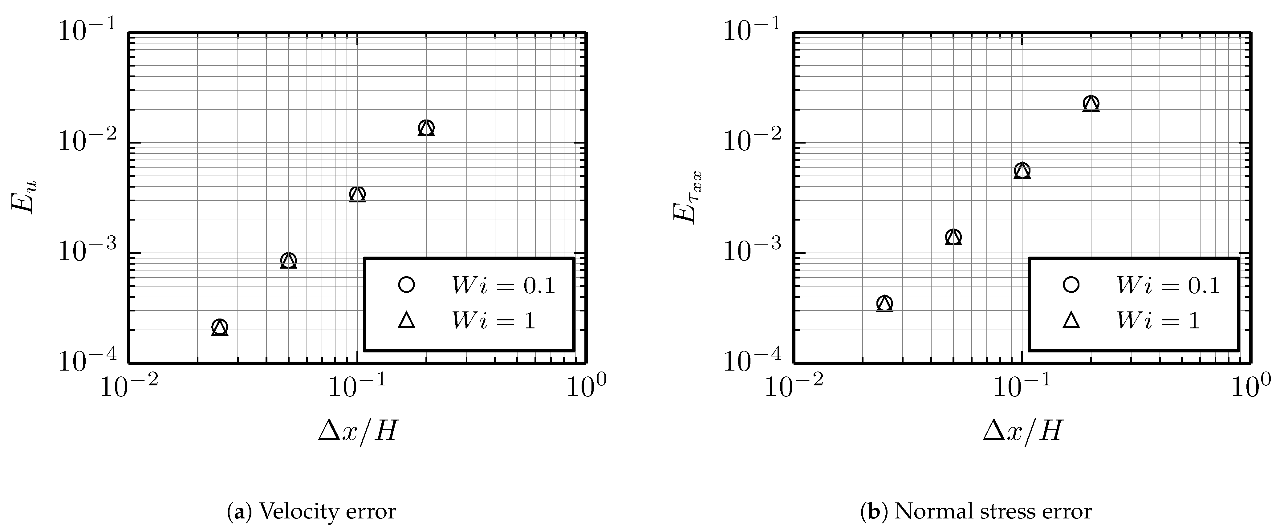
The error measurements with respect to the analytic steady state solution are calculated as

$$E_{\varphi }=\frac{{\left|\left|{\varphi }_s-{\varphi }_a\right|\right|}_{L_2}}{{\left|\left|{\varphi }_a\right|\right|}_{L_2}},$$

(25)

where ${\varphi }_s$ and ${\varphi }_a$ denote the simulated and analytic solution, respectively. The computed errors for velocity and viscoelastic normal stress are shown as a function of grid size in Figure 7. The errors decrease with second order slope with grid refinements, which is coherent with the second order accuracy that was observed for the original Lagrangian–Eulerian method [27,28].

4.2. Die Swell

The die swell effect is a phenomenon that occurs for the free surface flows of viscoelastic fluids flowing in a pipe or channel and exiting through circular or slit dies. Barnes et al. [47] described the origin of the die swell effect by viewing the viscoelastic fluid as a bundle of elastic threads. In the channel flow, the threads are stretched by the normal stress component ${\tau }_{xx}$, where x is the flow direction. When the fluid exits the channel, the threads are allowed to relax and shorten in length. Consequently, the diameter of the emerging fluid increases.

Flows that exhibit the die swell effect are commonly used to benchmark and validate numerical methods [11,13,14,16,17,18,19,20,22,24]. In addition to the free surface, the flow has extensional characteristics around the channel exit as well as a stress singularity at the channel exit corner. These flow features make the flow suitable for testing robustness and accuracy of new numerical methods. Therefore, in this work, a planar die swell flow is simulated. The case parameters are selected to allow for a meaningful comparison with numerical data from the literature.

A schematic description of the computational domain can be found in Figure 8. A channel of height $2h$ and length $10h$ is considered. A symmetry boundary condition is used at $y=0$, such that effectively half of the domain is simulated. The expansion zone is $5h$ high and $12h$ long, giving the domain a total length of $22h$. The length of the channel and size of the expansion zone are chosen to be sufficiently large for boundary effects not to affect the flow near the channel exit.

The exterior boundaries of the expansion zones are treated as outlets with the pressure condition $p=0$, and an immersed boundary is used to impose the no-slip condition for the channel walls. Gravity is neglected.

The viscoelastic fluid in the channel is an Oldroyd-B fluid with the viscosity ratio $\beta =1/9$. The surrounding fluid is a Newtonian fluid with much lower viscosity and density than the viscoelastic fluid. In this work, these parameters are set to ${\mu }_{\mathrm{air}}={10}^{-6}\mu$ and ${\rho }_{\mathrm{air}}={10}^{-3}\rho$, respectively. Comminal et al. used a similar definition [24], but with ${\rho }_{\mathrm{air}}={10}^{-2}\rho$.

The simulation of the flow starts from rest, with the channel filled with viscoelastic fluid. Transient flow is simulated for a sufficiently long physical time for the flow in the channel and the expansion region to fully develop, as well as for the free surface flow to exit through the outlet with a uniform velocity profile.

At the inlet, fully developed flows are imposed for the velocity and viscoelastic stress. For fully developed channel flow of an Oldroyd-B fluid, it can be shown that

$$u\left(y\right)=\frac{3}{2}U\left(1-\frac{y^2}{h^2}\right),$$

(26)

$$\frac{\partial u}{\partial y}=-\frac{3Uy}{h^2},$$

(27)

$${\tau }_{xy}\left(y\right)=\eta \frac{\partial u}{\partial y},$$

(28)

$${\tau }_{xx}\left(y\right)=2\lambda {\tau }_{xy}\left(y\right)\frac{\partial u}{\partial y}=2\lambda \eta {\left(\frac{\partial u}{\partial y}\right)}^2,$$

(29)

where U is the mean velocity. A derivation of the expressions can be found in Appendix A.

The channel half height h and velocity U are taken as characteristic length and velocity scales for the flow. Thus, a Weissenberg number for the flow may be defined as

$$\mathrm{Wi}=\frac{\lambda U}{h},$$

(30)

and a Reynolds number as

$$\mathrm{Re}=\frac{2\rho Uh}{\mu +\eta }.$$

(31)

A dimensionless time is also defined as $t^{*}=tU/h$.

The swell ratio $S_r=h_{max}/h$ is the main quantity of interest, in terms of validation by comparison. The swell ratio is a function of the so-called recoverable shear $S_R$, which is defined as [11]

$$S_R={\left|\frac{N_1}{2{\tau }_{xy}}\right|}_{y=h}={\left|\frac{{\tau }_{xx}-{\tau }_{yy}}{{\tau }_{xy}}\right|}_{y=h}=\frac{3\lambda U}{h}=3\mathrm{Wi},$$

(32)

where $N_1={\tau }_{xx}-{\tau }_{yy}$ is the first normal stress difference. In the simulations that are reported in this section, the quantities U, $\eta$, $\mu$, and $\rho$ are constant, while $S_R$ is varied by changing $\lambda$ between simulations. The Reynolds number is $\mathrm{Re}=0.5$ for all simulations.

Tanner [48,49] developed a theoretical solution for the amplitude of the die swell as a function of the recoverable shear. For an Oldroyd-B channel emerging from a slit the solution reads

$$S_r=0.19+{\left(1+\frac{{S_R}^2}{3}\right)}^{\frac{1}{4}}.$$

(33)

The theory does not take the stress singularity at the channel exit corner into account and is, therefore, only expected to yield a good approximation of the swell ratio when the influence of elasticity is small, i.e., for small Wi. Nevertheless, it is often included for comparison in numerical studies of the die swell effect and it is included in this study.

The influence of the spatial discretization on the numerical results is assessed through a grid dependence study and the flow is simulated for $S_R=2.5$ with three different grids, denoted as M1, M2, and M3. A grid is defined by a base cell size $\Delta x_{\mathrm{base}}$ and a set of refinements, as described in Section 3. The grids M1, M2, and M3, respectively, have the base cell sizes $\Delta x_{\mathrm{base}}=h/5,h/10,h/20$. The largest cells are located in the expansion zone, far from the channel exit. One level of refinement is used in the channel and around the channel opening and two levels of refinement near the exit corner. As an example, grid M1 is shown in Figure 9. The area around the channel exit corner has been zoomed for clarity.

Table 1. Summary of grids that are used to study the grid dependence of the die swell simulations.

Grid	$\mathit{h}/\Delta {\mathit{x}}_{\mathbf{base}}$	$\mathit{h}/\Delta {\mathit{x}}_{\mathbf{channel}}$	$\mathit{h}/\Delta {\mathit{x}}_{\mathbf{corner}}$	Num. Cells Total.
M1	5	10	20	4829
M2	10	20	40	19,685
M3	20	40	80	78,740

summarizes the grids used. A constant time step length is used, such that $U\Delta t/\Delta x_{min}=0.01$, where $\Delta x_{min}$ is the smallest cell size of the grid.

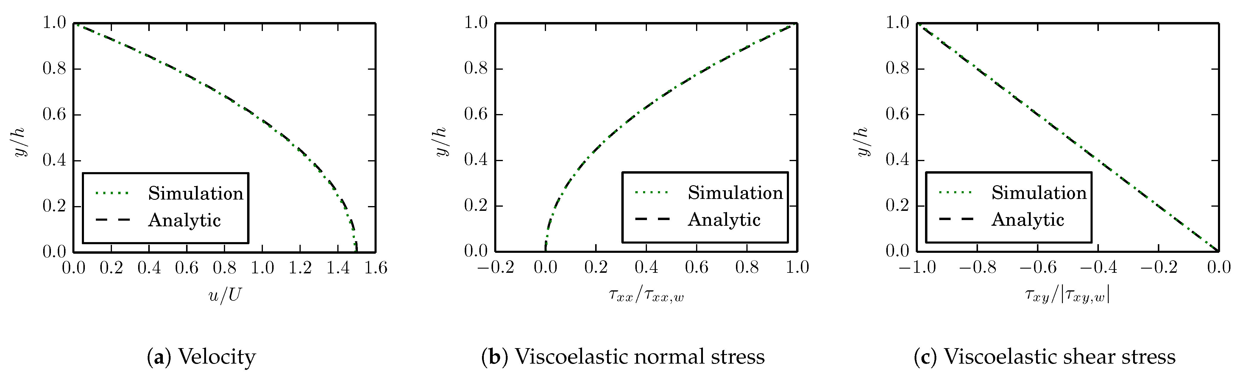
First, the velocity as well as the viscoelastic normal and shear stress are compared to the analytic steady solution inside the channel. In Figure 10, the corresponding profiles obtained using grid M1 across the channel at $x/h=5$, halfway from the inlet to the channel exit. Already at the lowest grid resolution, the simulated profiles overlap the analytic solution. The results that are obtained with M2 and M3 are visually the same and the figures are, therefore, omitted. The results validate that the constitutive equations are solved correctly and that the immersed boundary method used to impose the boundary conditions at the channel wall works as intended for the solution algorithm for the viscoelastic stresses.

In Figure 11, the position of the free surface that is visualized by the contour $\alpha =0.5$ is shown for $S_R=2.5$ for the grids that are defined in Table 1. Some small surface oscillations are observed in the results from the two finer grids M2 and M3 in the region $x/h<2$. As reference, Comminal et al. [24] reported similar behavior for their corresponding simulations. In their simulations, small self-sustained surface oscillations appeared at a certain level of recoverable shear, in their case $S_R>1.5$ for the Oldroyd-B fluid, and for sufficiently high resolution. Similar observations were also made for simulations with the Giesekus model in their study. The oscillations were damped out further downstream and they did not influence the calculated swell ratio $h_{max}/h$. Similar characteristics are observed in the current work, as in Figure 11. Comminal et al. attributed the oscillations to numerical difficulties around the free surface due to the nature of the non-sharp interface in the VOF method.

In the light of this discussion, the results that are obtained on grid M2 and M3 are in relatively good agreement. This is particularly true far downstream of the channel exit, where the free surface produced by M2 and M3 are very close, while M1 produces a different result. The results indicate that M2 is of sufficient spatial resolution to predict the swell ratio $S_r$. Therefore, the results presented in the remainder of this section have been obtained while using grid M2. In addition, the simulation with grid M2 has been repeated with half the time step size, such that $U\Delta t/\Delta x_{min}=0.005$, which produced equivalent results.

The simulations are repeated with grid M2 for $S_R\in \{1.0,1.5,2.0,2.5\}$. In Figure 12, the contour $\alpha =0.5$ is shown for $S_R=1$ at different times. Figure 13 shows the corresponding results for $S_R=2.5$. Similar behavior is observed in both cases. The emerging viscoelastic fluid increases in diameter directly upon exiting the channel. The magnitude of the increase is strongly influenced by the level of elasticity, as qualitatively predicted by Tanners theory. At a certain distance from the channel exit, approximately for $x/h>3$, the emerging viscoelastic fluid reaches a terminal diameter.

The swell ratio is calculated for the simulations as $S_r=h_{max}/h$, where $h_{max}$ is taken as the position of the free surface at $x/10$. The calculated swell ratios that were obtained with the proposed method are compared to available numerical data from the literature. The data used are the original FEM simulations reported by Crochet and Keunings [11], the marker-and-cell simulations by Tomé et al. [14], the pseudo-VOF simulation by Habla et al. [22], and the three different VOF methods used by Comminal et al. [24].

Table 2. Summary of numerical data as compared for the die swell flow.

Work	Method	Re
Current work	VOF, Lagrangian-Eulerian	$0.5$
Crochet & Keunings [11]	Mixed FEM	0
Tomé et al. [14]	GENSMAC	$0.5$
Habla et al. [22]	pseudo-VOF	$0.5$
Comminal et al. [24] (CCU)	VOF, Geometric scheme	0
Comminal et al. [24] (HRIC)	VOF, Algebraic scheme	0
Comminal et al. [24] (RheoTool)	VOF, Algebraic scheme (MULES)	$0.01$

briefly summarizes the data. For a full description of the cases and numerical methods, the reader is referred to the respective studies. However, a brief discussion concerning the differences between the results is given below.

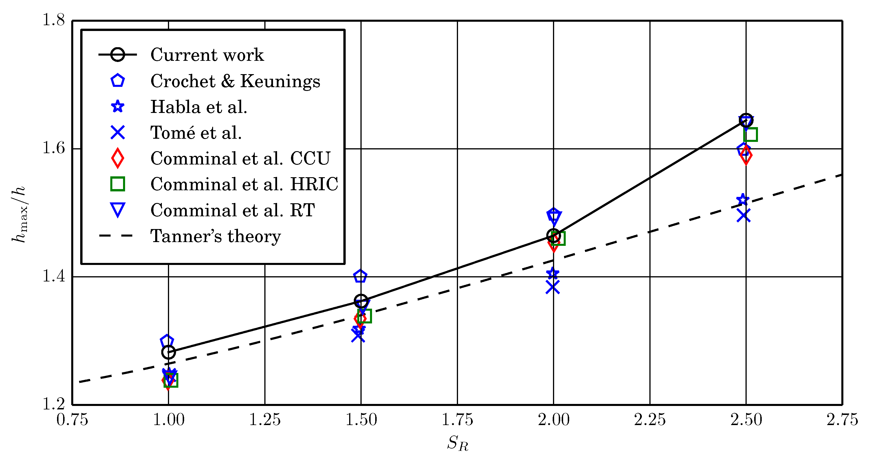
The calculated swell ratios as a function of the recoverable shear for the flows simulated with the proposed method are compared to the results from the literature in Figure 14. It is remarked that Comminal et al. employed a different definition of the Weissenberg number and swell ratio. However, all of the data that are presented in Figure 14 have been adopted to the definition used in the current work.

Indeed, a certain spread among the data is observed. The differences are not unexpected, though, as there are slight differences between how the different data have been obtained. This is in terms of the numerical method used as well as the simulation setup. Furthermore, Comminal et al. even obtained different results while using three slightly different numerical methods for exactly the same flow.

Crochet and Keunings and Tomé et al. did not consider a fluid surrounding the viscoelastic phase, as the per construction of their numerical methods. Comminal et al. used a similar definition of the surrounding fluid as in the current work, but with larger density. Habla et al. stated that the surrounding fluid is treated as air with ${\mu }_{\mathrm{air}}\to 0$ and ${\rho }_{\mathrm{air}}\to 0$, but the magnitudes were not reported. Furthermore, the value of viscosity ratio of the viscoelastic fluid $\beta$ varied between their simulations. This is in contrast to a constant $\beta =1/9$, which has been used in the other simulations included in this work.

Given the above discussion, a certain variance in the data is to be expected. However, the different results do follow the same general trend, including the swell ratios predicted with the proposed Lagrangian–Eulerian method.

Another aspect is that of grid dependence. The simulation performed by Crochet and Keunings had a grid resolution which, by today’s standards, was very coarse. They used six triangular finite elements across the half-width of the channel. Therefore, the resulting swell ratios should be treated with caution when comparing to more recent results. Tomé et al. used a uniform grid of $\Delta x/h=1/10$ which is on the order of the coarse grid M1. Habla et al. reported the number of control volumes to be 4165, but did not specify the local cell sizes in detail. The number of control volumes is again comparable to grid M1 in the current work. Comminal et al. did conduct a grid dependence study with three different grids. Their finest cells were closer to the grids that were used in this work as compared to the other authors. Therefore, could be expected for the results reported in this work to be closest to the results of Comminal et al. given the similarities in grid resolution as well as the use of the VOF method. Their computed swell ratios are generally larger than the other literature results, with the exception of those from Crochet and Keunings. The same is also true for the swell ratios that were computed with the proposed method, particularly for increasing $S_R$.

In conclusion, while there is a spread between the data that are produced in different numerical studies, they follow the same general trend. The results that were obtained with the method proposed in this work follow the same trend and with the swell ratios comparable to the earlier published works.

4.3. Jet Buckling

The simulation of jet buckling is a common flow case for testing the capabilities of numerical methods for free surface flow. The phenomenon has been numerically investigated for different viscoelastic constitutive models by several authors [14,15,16,17,18,20,26].

The phenomenon occurs for a fluid jet that flows onto a rigid plate under certain conditions. Cruickshank [50] proposed a condition that is based on experimental and theoretical observations, stating that a planar Newtonian jet will buckle if $H/D>3\pi$ and $\mathrm{Re}<0.56$, where H is the distance from the inlet to the plate, D the inlet width, and $\mathrm{Re}=\rho UD/\mu$, where U is the inlet velocity. A modified yet approximate condition, based on numerical investigation, was later proposed by Tomé and McKee, stating that buckling should occur if

$${\mathrm{Re}}^2\le \frac{1}{\pi }\frac{{(H/D)}^{2.6}-8.8^{2.6}}{{(H/D)}^{2.6}}.$$

(34)

It is remarked that, in simulations, numerical round-off errors are responsible for triggering the buckling, since the flow setup itself is actually symmetric.

Figure 15 shows a schematic of the fluid jet buckling domain that is used for simulation with the Lagrangian–Eulerian method proposed in this work. The domain is 50 mm wide and 100 mm high. An inlet of width $D=5\mathrm{mm}$ is located at the center of the upper boundary. At the inlet, a uniform velocity $U=0.5\mathrm{m}/\mathrm{s}$ is imposed. The upper boundaries to the left and right, respectively, are outlets with the Dirichlet pressure condition $p=0$. The remaining domain boundaries are treated as walls by imposing the no-slip condition. Gravity is acting in the negative y-direction with $g=9.81\mathrm{m}/{\mathrm{s}}^2$.

The viscoelastic fluid is a single-mode Oldroyd-B fluid with the viscosity ratio $\beta =0.1$, density $\rho =1000\mathrm{kg}/{\mathrm{m}}^3$, and the total viscosity ${\eta }_t=10\mathrm{Pa}·\mathrm{s}$. The surrounding Newtonian viscosity is air with viscosity ${\mu }_{\mathrm{air}}=1.8205\times {10}^{-5}\mathrm{Pa}·\mathrm{s}$ and density ${\rho }_{\mathrm{air}}=1.204\mathrm{kg}/{\mathrm{m}}^3$.

The Reynolds number for the flow is defined as $\mathrm{Re}=\rho UD/(\mu +\eta )$, which, for the chosen parameters, yields $\mathrm{Re}=0.25$. A Weissenberg number is defined as $\mathrm{Wi}=\lambda U/D$. The flow is simulated for the Oldroyd-B fluid with $\lambda =0.1\mathrm{s}$, corresponding $\mathrm{Wi}=10$. As reference, a simulation is also performed with a Newtonian fluid, for which $\beta =\mathrm{Wi}=0$.

In the viscoelastic jet buckling simulations that were performed in this work, the octree grid is adaptively refined with two levels around the viscoelastic fluid phase. As the simulation progresses, the grid is therefore updated and the cells are refined and coarsened, where needed. A grid dependence study is performed while using three adaptive grids of increasing resolution. The grids have the respective base cell sizes $\Delta x_{\mathrm{base}}=D/2,D/4,D/8$, which correspond to the finest cell sizes $\Delta x_{min}=D/8,D/16,D/32$. The simulations are performed with a constant time step $\Delta t$ satisfying $\Delta tU/\Delta x_{min}=0.08$.

The grid dependence is evaluated with respect to two simulation properties. Firstly, the free surface $\alpha =0.5$ is compared for the three adaptive grids. The first normal stress difference $N_1={\tau }_{yy}-{\tau }_{xx}$ along the jet at $x=5D$ is also compared. Because the buckling itself is triggered by numerical round-off errors, the exact conditions at which the buckling starts in the simulations may vary between grids. Therefore, the grid study comparison is made at a simulation time before buckling is initiated.

In Figure 16, the free surface is compared for the three grids at the simulation times $t=130\mathrm{ms}$ and $t=140\mathrm{ms}$. The results obtained with the three grids are in relatively good agreement, particularly those that are obtained with the two finer grids. In Figure 17, the first normal stress differences along the jet are compared at the same simulation times. These results indicate even more strongly that the two finer grids produce stresses that are very close, while a slight discrepancy for the coarsest grid is observed. The remainder of the results reported in this section have been obtained while using $\Delta x_{min}=D/16$.

In Figure 18 and Figure 19, a series of snapshots from the simulation of the Newtonian and the viscoelastic jets are shown, respectively. For the Newtonian case, only a very slight tendency to buckle is observed as a slight asymmetry in the fluid on the rigid surface. However, for the viscoelastic fluid, the buckling phenomenon is very apparent. When the viscoelastic jet impacts the rigid surface, the material first builds upwards until, inevitably, the buckling is initiated. The results demonstrate the strong influence of elasticity to the fluid jet buckling phenomenon. Furthermore, it confirms the capability of the proposed method to capture the viscoelastic effects and predict the phenomenon.

5. Conclusions

In this work, a new Lagrangian–Eulerian method for the simulation of viscoelastic free surface flow has been proposed. The method was developed from a previously proposed method, in which the fluid momentum and continuity equations were solved on a stationary Eulerian octree grid, while the viscoelastic constitutive equation was solved along the trajectories of Lagrangian nodes which were convected by the flow. The main improvements in this work was the introduction of a backwards-tracking procedure for solving the viscoelastic constitutive equation, as well an extension to the simulation of viscoelastic free surface flow with the volume of fluid method.

The backwards-tracking procedure allowed for the storage of the viscoelastic stresses in a structured arrangement. Consequently, the unstructured interpolation of stresses as well as the addition and deletion of Lagrangian nodes, which was required in the previous method, was eliminated in favor of a significant reduction of the computational cost and increased robustness. Furthermore, no additional stabilization method, such as both sides diffusion or reformulation of the constitutive equation, was employed for any of the flows studied in this work.

The proposed method was validated with analytic solutions for a planar Poiseuille flow of Oldroyd-B fluids. The transient, as well steady flow, solutions were in excellent agreement with analytic solutions and the steady solution converged to the analytic solution with second order accuracy. Furthermore, the proposed method was evaluated for two types of viscoelastic free surface flow. The viscoelastic die swell effect was simulated with the Oldroyd-B model and the predicted swell ratios were in good agreement with the numerical data from the literature. Planar jet buckling of a highly viscoelastic fluid was also simulated, demonstrating the capability of the method for an additional flow case as well as the use of adaptive grid refinements.

The computational performance was not subject to detailed study in this work. However, as per the construction of the new method, the computational cost for the viscoelastic stress calculation was significantly reduced when compared to the previous Lagrangian–Eulerian method. Furthermore, it has previously been shown that the Lagrangian formulation of the constitutive equation is highly suitable for parallel calculations, including for GPU-acceleration. This also applies for the new method.

In conclusion, the new method is an important step in the development of efficient and useful tools for simulating industrial processes involving viscoelastic fluids. In future research, the proposed Lagrangian–Eulerian method will be used for the numerical investigation of viscoelastic free surface flows with moving objects, including for viscoelastic adhesive application and parts assembly, as well as for additive manufacturing processes.