1. Introduction
As modern software is getting more complex, it is of great importance to ensure software reliability. Up to now, the most practical way of building high-reliable software is via a huge amount of testing and debugging. Therefore, software defect prediction, a technique to predict defects in software artifacts, has gained popularity by lessening the burden of developers to prioritize their testing and debugging efforts [
1].
For decades, hand-crafted metrics have been used in software defect prediction. Since AlexNet [
2], deep learning has been growing rapidly in image recognition, speech recognition, and natural language processing [
3]. The same trend also appears in software defect prediction because deep learning models are more capable of extracting information from long texts, i.e., source code. Instead of using hand-crafted metrics that are designed top-down, deep learning models are able to generate code features bottom-up from source code and could describe both syntax and semantic information. Many researchers [
4,
5,
6,
7,
8,
9,
10,
11,
12,
13,
14,
15,
16,
17,
18,
19,
20,
21,
22,
23,
24,
25] use various kinds of deep learning models, e.g., Convolutional Neural Networks (CNN), Long-short Term Memory (LSTM) models, and Transformers for software defect prediction, and achieve promising results. However, due to the limited dataset size in software defect prediction (compared to massive lines of source code directly available in open source repositories), it is hard to believe that a deep learning model trained for software defect prediction can really “understand” the source code itself. Therefore, two problems arise.
Can we use a model that “understands” source code for software defect prediction? How should we use such a model for software defect prediction?The language model, a core concept in natural language processing, is gaining popularity. The reason is that, given the abundance of natural language corpora, and the difficulty of getting labels for prediction tasks, it is more economic-efficient to fully leverage the original corpora in an unsupervised fashion before the language model is later used in other prediction tasks. There are many popular language models such as Word2Vec [
26] and Glove [
27]. Recently in 2019, BERT [
28] improves natural language pre-training using mask-based objectives and a Transformer-based architecture. BERT has successfully improved many state-of-the-art results for various natural language tasks.
Along with the development of the natural language model, recent research also shows great success in applying natural language models to artificial languages, especially programming languages. Such programming language models mainly embed local and global context [
29], abstract syntax trees (ASTs) [
30,
31], AST paths [
32], memory heap graphs [
33], and the combination of ASTs and data-flows [
34,
35]. CodeBERT [
36] is one of the latest released powerful language models that is a transformer pre-trained with a Bert-like architecture on open source repositories. It could support paired natural language and multi-lingual programming language tasks, such as code search and code documentation generation. Despite the great success of fine-tuning CodeBERT in downstream tasks, it remains unclear if CodeBERT could improve results in software defect prediction.
In this paper, we investigate the feasibility of using the CodeBERT model for software defect prediction. Specifically, we propose four models based on CodeBERT: CodeBERT-NT, CodeBERT-PT, CodeBERT-PS, and CodeBERT-PK. We perform experiments to investigate the performance of CodeBERT-based models that “understand” source code syntax and semantic and design new prediction patterns that are specially designed for pre-trained language models like CodeBERT. The experimental data are available at
https://gitee.com/penguinc/applsci-code-bert-defect-prediciton. (accessed on 23 May 2021).
Our contributions are as follows:
We are the first to introduce pre-trained programming language models for software defect prediction.
We propose new forms of prediction patterns specially designed for pre-trained language models in software defect prediction.
We discuss the reason why new forms of prediction patterns work in software defect prediction.
2. Background
2.1. Deep Learning Based Software Defect Prediction
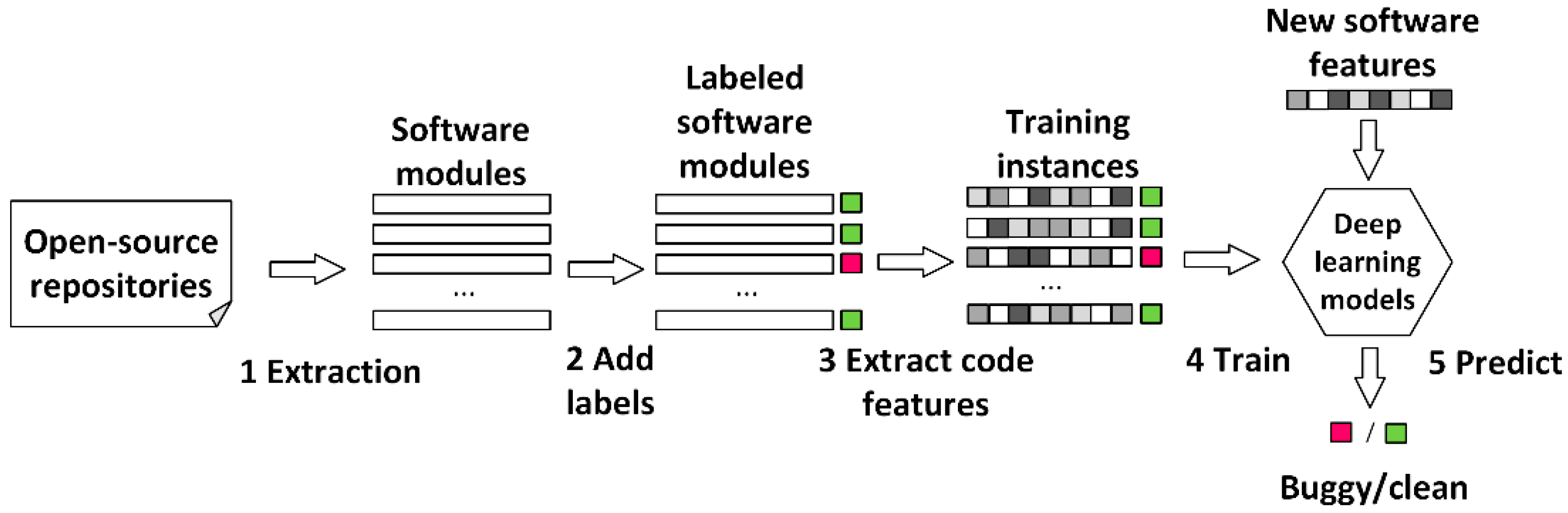
Figure 1 shows a typical workflow of deep learning-based software defect prediction. The first step is to extract software modules from open-source repositories. A software module could be a method, a class, a file, a code change, etc. The second step is to mark software modules as buggy/clean. The bug information is extracted from post-release defects recorded in bug tracking systems, e.g., Bugzilla. If a software module contains bugs found in later releases, the module is marked as buggy. The third step is to extract code features from software modules. In deep learning-based software defect prediction, typical code features include character-based, token-based, AST-node-based, AST-tree-based, AST-path-based, and AST-graph-based features. The fourth step is to build a deep learning model to generate features and train the instances. Frequently used deep learning models in software defect prediction include CNN, LSTM, Transformers, etc. The last step is to use the trained deep learning model for inference, i.e., predict whether a software module is buggy or clean.
Deep learning-based software defect prediction can be organized into two categories:
Software defect prediction based on deep learning and hand-crafted features. Deep learning is expert at combining hand-crafted features. Therefore, hand-crafted features can be fed into deep learning models to improve prediction performance. Yang et al. [
37] are the first to use fully connected neural networks for hand-crafted feature combinations. Other deep learning models include autoencoders [
38,
39] and ladder networks [
39]. The results show that deep representations of hand-crafted features could further improve prediction performance compared to experiments using traditional machine learning models and hand-crafted features.
Software defect prediction based on deep learning and generated features. With the rapid progress in the natural language processing domain, deep learning models are capable of processing long texts, e.g., source code. Unlike designed top-down hand-crafted features, the features are generated bottom-up from the source code, which could represent structural and semantics information of the source code. Recently, many deep learning models, including Deep Belief Networks [
4,
15], CNN [
5,
6,
7,
10,
17,
19,
24,
25], LSTM [
11,
12,
14,
16,
18], Transformers [
8], and other deep learning models [
13,
22] are used in software defect prediction.
Researchers also explore more efficient ways of source code representations. Most researchers use AST sequence to represent source code [
4,
5,
7,
17] which balances the information density represented and the training difficulty of deep learning models given insufficient datasets. Some researchers also present representations based on AST paths, e.g., PathPair2Vec [
9] and Code2Vec [
32]. AST paths could extract node-path information that is not shown in AST sequences at the cost of the explosion of path numbers and training efforts. Other researchers explore context information based on AST sequences to focus on defect characteristics [
19].
2.2. Deep Transfer Learning
In some domains, including software defect prediction, it is challenging to construct a large-scale, high-quality dataset due to the high cost of labeling data samples. Transfer learning, which assumes that training data do not have to be identically distributed (i.i.d.) with test data, could mitigate the problem of insufficient training data [
40].
The definition of transfer learning is proposed by Tan et al. [
41] as below. Given a learning task
based on
, and we can get help from
for the learning task
. Transfer learning aims to improve the performance of predictive function
for the learning task
by discovering and transferring latent knowledge from
and
, where
and/or
. In addition, in most cases, the size of
is much larger than the size of
,
.
Deep transfer learning is a special form of transfer learning that uses a non-linear deep learning model for transfer learning [
41]. Deep transfer learning can be organized into four categories: instance-based deep transfer learning, which uses instances in source domain by appropriate weights; mapping-based deep transfer learning, which maps instances from two domains into a new data space with better similarity; network-based deep transfer learning, which reuses the parts of the network pre-trained in the source domain; and adversarial-based deep transfer learning, which uses adversarial learning to find transferable features that are both suitable for both domains. Among the four methods, network-based deep transfer learning is generally accepted by researchers and has been practically used in many domains. For example, researchers could use pre-trained models published by large IT companies like Google and Facebook and fine-tune the model via deep transfer learning to adapt to downstream tasks. More recently, pre-training language models with large amounts of unlabeled data and fine-tuning in downstream tasks have made a breakthrough in the natural language processing domain, such as OpenAI GPT and BERT [
28].
A typical process of network-based deep transfer learning is shown in
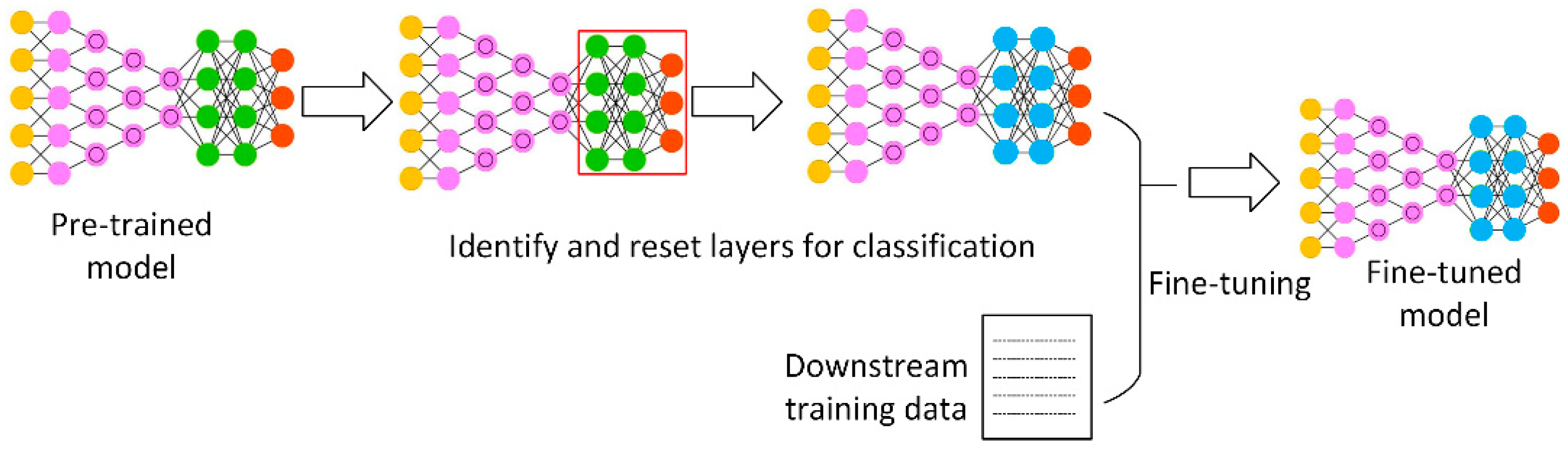
Figure 2. First, a pre-trained deep learning model is downloaded and available for fine-tuning. The weights are reserved in a pre-trained model. Second, the last layers of the pre-training deep learning models are identified, and the existing weights of these layers are removed. It is assumed that a pre-trained model contains two parts: general knowledge embedding layers and classification layers that target a specific upstream task, e.g., masked language model for text processing. It is generally accepted to reset the weights of the classification layers so that the model remains common knowledge, whereas it could be generalized to downstream tasks, e.g., text classification. Third, the downstream training data, which is usually much small than the dataset to train the pre-trained model up to several orders of magnitude, are fed to the model, which is called the fine-tuning process. During the process, the model learns how to perform downstream prediction tasks based on both pieces of knowledges from the pre-trained model and the downstream training data. Last, the fine-tuned model is available for downstream prediction tasks.
Deep transfer learning requires that the upstream and downstream tasks are transferrable. For example, suppose we use a pre-trained model on text generation (e.g., text corpora form Wikipedia) and use the model for text sentiment classification (e.g., whether a sentence is positive or negative). In that case, the tasks are transferrable because such models will classify a sentence as positive or negative based on both keywords like fantastic and awful, and the whole meaning of the sentence, e.g., a rhetorical question could entirely divert the meaning of a sentence.
2.3. BERT and CodeBERT
Language models can be roughly categorized into N-gram language models and neural language models. Classical neural language models include Word2Vec [
26] and Glove [
27], which are still popular in software defect prediction [
4,
5,
7]. BERT [
28] improves natural language pre-training by using mask-based objectives and a Transformer-based architecture, which has successfully improved many state-of-the-art results for various natural language tasks. It is one of the best pre-training language models for downstream tasks, considering that more powerful models (e.g., GPT3 [
42]) are not open-source and not easily accessible. RoBERTa [
43] is a replication of the BERT paper which follows BERT’s structure and proposes an improved pre-training procedure. CodeBERT [
36] follows the architecture of BERT and RoBERTa, i.e., the RoBERTa-large architecture. Unlike BERT and RoBERTa, which target natural languages, CodeBERT utilizes both natural languages and source codes as its input.
The overall architecture of BERT is shown in
Figure 3. The core blocks in BERT are Transformers [
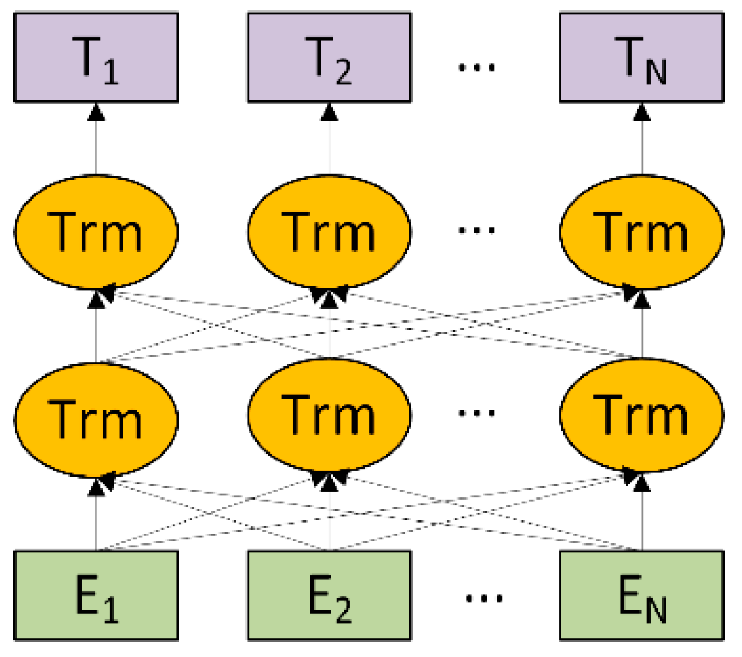
44], which follow an encoder-decoder architecture. Based on the attention mechanism, Transformers could convert the distance of any two words in a sentence to 1, which mitigates the long-term dependency problems in natural language processing. The input corpora are first encoded into feature vectors via multi-head attention and fully connected layers. Then, the feature vectors are fed to the decoder, which includes masked multi-head attention, multi-head attention, and fully connected layers, and are finally converted to the conditional probabilities for prediction. Unlike the OpenAI GPT model, BERT uses a bidirectional Transformer that enables extracting context from both directions.
Since we do not change the architecture of CodeBERT, the formulas of the CodeBERT model, BERT model, RoBERTa model, and Transformers model are omitted for simplicity.
3. Motivation
3.1. Proving the Naturalness Assumption via Language Models in Software Defect Prediction
The use of language models greatly speeds up the advancements in natural language processing. In terms of the software engineering domain, there is usually a few years gap between the time a new language model is proposed and the time it is used in this domain. For example, the use of Word2Vec and Glove is still popular in software defect prediction. Similarly, since the breakthrough of the natural language processing domain (the BERT model) is proposed in 2019, it is not until last year before CodeBERT, a pre-trained programming language model using the BERT architecture, is proposed, and the model is open to the public.
It is yet unclear whether using a pre-trained language model will improve the prediction performance of software defect prediction. Since naturalness has been regarded as an essential part of code characteristics [
45,
46], researchers would assume that a large-scale programming language model would be more competent in identifying “unnatural” code, i.e., code that does not follow the universal patterns identified from large code corpora. Recently, the naturalness assumption has been proven by IBM researchers by tagging AST nodes via pre-trained language models [
47]. The naturalness assumption indicates that “unnatural” codes are more likely to be buggy when it comes to software defect prediction. However, it remains unclear whether the naturalness assumption is valid in software defect prediction.
3.2. The Influence of Prediction Patterns in Software Defect Prediction
The traditional software defect prediction pattern is to predict whether there are software defects in the source code. Specifically, given the features generated from machine learning models, software defect prediction aims to predict 0 for clean code and 1 for buggy code. During the process, a prediction model will not be aware that it performs defect prediction. Assume that we tell the model that it is performing software defect prediction tasks by some means; the model is expected to directly link the textual concept of defects to the semantic parts expressed by natural languages in the source code. Unlike the traditional prediction pattern that takes only code semantics into account, the new prediction pattern also considers textual semantics. For example, if a function is named “Workaround” and the function is unnaturally complex, a model could judge from textual semantics that a historical bug may not be fully solved and may reoccur in the future, and judge from code semantics that a function with very high complexity may be more likely to be buggy. It is worth noting that the new prediction patterns require that the model is a programming language model that understands both natural language and programming language, e.g., CodeBERT.
4. Approach
4.1. Workflow
The workflow of our approach is shown in
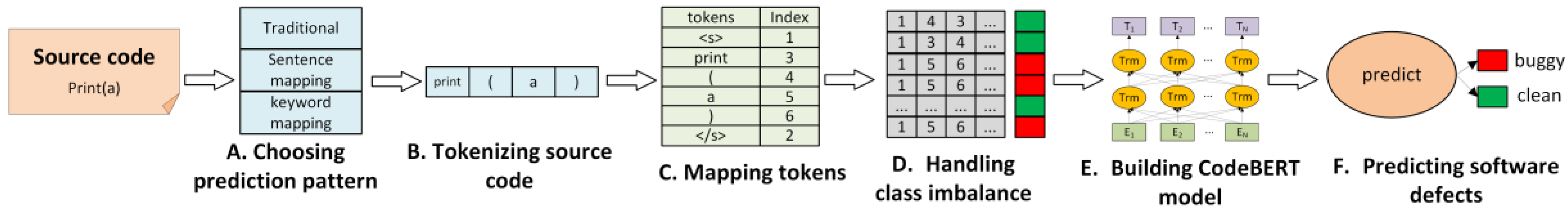
Figure 4. The approach consists of six steps. In step A, different prediction patterns are chosen, which influences the components of the input data. In step B, the source code is tokenized into tokens, guided by the grammar rules in Backus Normal Form. In step C, the tokens are mapped to integer indexes, and some special tokens are also added. In step D, a simple class balancing method is applied to the indexed tokens. In step E, we feed the balanced data to a CodeBERT model based on model data available at the HuggingFace website [
48]. Finally, in step F, we predict a new source file as buggy or clean using the trained CodeBERT model.
4.2. Choosing Prediction Pattern
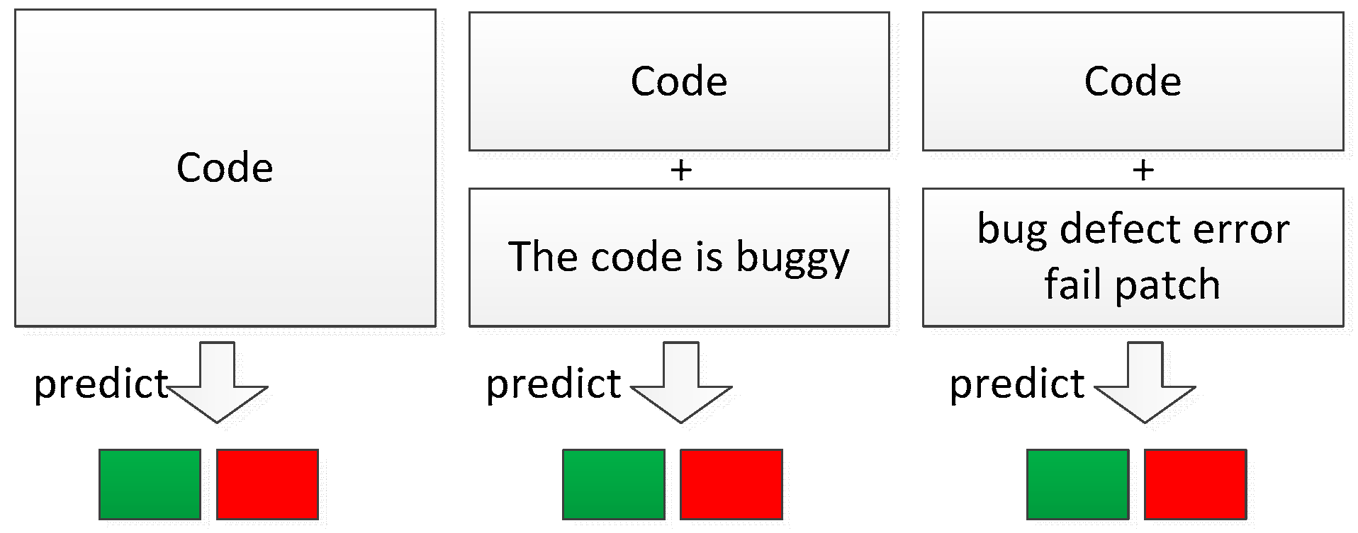
This paper uses three prediction patterns for software defect prediction, which originates from motivation 2 in the previous section, as shown in
Figure 5. The first prediction pattern is the most commonly used pattern that takes the source code as inputs and predicts 0 for clean code and 1 for buggy code. The second prediction pattern takes both the source code and a declarative sentence (e.g., “The code is buggy”) as inputs and predicts 0 if the declarative sentence does not match the source code (i.e., the code is clean) or predicts 1 otherwise. In this case, the declarative sentence is more like a question answered with 0 or 1. The third prediction pattern takes both the source code and a list of keywords (e.g., bug, defect, error, fail, patch) as inputs and predicts 0 if the keyword list does not match the source code (i.e., the code is clean), or predicts 1 otherwise. The second and the third prediction pattern is very similar, despite that the second prediction pattern requires more textual comprehension of the declarative sentence, while the third prediction pattern could lessen the burden of textual comprehension by leveraging keyword search and mapping.
In the following sections, we name the first prediction pattern as “traditional”, the second prediction patter as “sentence”, and the third prediction pattern as “keyword” for simplicity.
4.3. Tokenizing Source Code
During the compilation of the source code, a normal tokenizer that separates the tokens following grammar rules is sufficient. However, as is usually neglected during compilation, the semantics hidden in texts, e.g., function names and variable names, are often neglected. Therefore, a tokenizer that could extract the text semantics in source code should be used.
We follow the settings of CodeBERT, which uses a word piece tokenizer. Before the original source code is fed into the word piece tokenizer, code comments are removed, the white spaces at the head and the tail of the source code are removed, the tokens are separated by splitting the white space, and the punctuations are also separated into independent tokens. This paper uses three preprocessing patterns for software defect prediction, which corresponds to the three prediction patterns described in
Section 4.2. The first preprocessing pattern (i.e., the traditional pattern) starts with a <s> mark at the beginning and </s> at the end. The second and the third preprocessing pattern (i.e., the sentence and keyword pattern) add an extra </s> mark to separate the source code and the declarative sentence or the keywords. The preprocessed code is then ready for tokenization.
During the tokenization process, the source code is tokenized using a pre-trained vocabulary file. The uncommon words are separated into several sub-words with higher occurrences in the vocabulary file using a greedy longest-match-first algorithm. For example, the word “TestCase” will be separated into “Test” and “##Case”. The “##” token marks that the token is a sub-word token. If a token is not found in the vocabulary file, an unknown token, <UNK>, will be used.
4.4. Mapping Tokens
The CodeBERT model provides a standardized tokenizer, BertTokenizer, that takes the preprocessed source code as input and outputs a list of integers. The BertTokenizer maps each token to an integer specified in the vocabulary file, including sub-word tokens, out-of-vocabulary tokens (<UNK>), and other special tokens (<s> and </s>). If padding is enabled, 0 will be padded before or after the generated integers to ensure that all generated integer lists have the same length.
4.5. Handling Class Imbalance
Class imbalance is common in software defect prediction because the buggy rate of a project is usually below 50%. We choose a simple class imbalance method, random oversampling, so that the training set is balanced, i.e., 50% buggy samples and 50% clean samples.
4.6. Loading Pre-Trained Model
The pre-trained CodeBERT model is published by researchers and is available online. There are two ways of using the CodeBERT model: reuse model weights or only reuse the model architecture. We experiment on both methods to investigate whether using pre-trained programming language models outperforms training a model with the same architecture from scratch. In the first method, we reuse weights of the encoder and decoder and clean the weights of the classification layers because we perform different tasks in pre-training and fine-tuning phases (software defect prediction VS neural code search). In the second method, we just reuse the RoBERTa-large model, which is adopted by CodeBERT.
Since we use pre-trained models, we do not aim to change most of the hyperparameters. Specifically, we use Transformer with six layers, 768-dimensional hidden states, and 12 attention heads as our decoder. We set the learning rate as 10−5, the batch size is 32, and the maximum epoch is 20. We tune hyperparameters and perform early stopping on the test set. The only difference, batch size, is due to the computational limitations.
4.7. Predicting Software Defects
After we feed the training set to the CodeBERT model, all parameters, including weights and biases, are fixed. Then, we ran the trained or fine-tuned CodeBERT model for each file in the test set to obtain prediction results. The results were in the form of a float number between zero and one, based on which we predicted a source file as buggy or clean. If the result was above 0.5, the prediction was regarded as buggy; otherwise, it was clean.
5. Experimental Setup
All of our experiments are run on a laptop with 5-holdouts repeated experiments.
5.1. Evaluation Metrics
We use four evaluation metrics to evaluate prediction performance, namely F-measure (F1), G-measure, area under curve (AUC), and Matthews correlation coefficient (MCC). These evaluation metrics are popular in software defect prediction and can comprehensively evaluate model capabilities.
F-measure is the most frequently used evaluation metric in software defect prediction. It highlights the prediction results on buggy samples and balances the precision and recall. Specifically,
F1 is the most common form of F-measure, which takes the harmonic average of precision and recall (also
TPR, true positive rate).
F1 is calculated as follows:
G-
measure is the harmonic mean of recall and true negative rate (
TNR). G-
measure targets the false alarm effects, which is of great importance in software defect prediction. G-
measure is calculated as follows:
AUC is a very important evaluation metric in many machine learning tasks. Unlike most evaluation metrics, AUC is not sensitive to the threshold settings, which inferencing an output ranging from 0 to 1 as buggy or clean. AUC is also not sensitive to class imbalance, which is often the case in software defect prediction.
MCC is a good evaluation metric for imbalanced datasets. It focuses on buggy and clean samples equally and describes the correlation between them.
MCC is calculated as follows:
In this paper, we regard F1 as the main evaluation metrics. We perform multiple experiments to find the experimental results with the best performance, i.e., best F1 values. The best performance of other metrics, including G-measure, MCC, and AUC values, are also recorded and shown online as supplementary data to our experimental results.
5.2. Evaluated Projects and Datasets
We use the PROMISE dataset [
49], which targets open-source software defect prediction. Specifically, we use the cross-version PROMISE source code (CVPSC) dataset for cross-version software defect prediction and the cross-project PROMISE source code (CPPSC) dataset for cross-project software defect prediction. Both the CVPSC and the CPPSC dataset include bug labels of specified versions of open source projects and the corresponding source code. Because the time cost of fine-tuning CodeBERT is not trivial, we choose seven project version pairs and nine project version pairs for CVPSC and CPPSC, respectively. Precisely, we follow the Pan et al.’s paper [
7] to set the CVPSC dataset and take the intersection of Shi et al.’s paper [
17] and the project versions in the CVPSC dataset to set the CPPSC dataset. Detailed information of the CVPSC and CPPSC dataset is shown in
Table 1 and
Table 2.
5.3. Baseline Models
Our paper aims to explore empirical findings on neural programming language models, i.e., CodeBERT models. As the CodeBERT model takes BertTokenizer to tokenize raw source code, which is very rare in software defect prediction, it is inappropriate to compare the results with other software defect prediction models based on ASTs, CFGs, and so on because their inputs vary. Since it is extremely time-consuming to train a new programming language model from scratch and published large-scale programming language models are very scarce, we do not take other programming language models into account when choosing baseline models. We choose the following six baseline models:
Pre-trained CodeBERT sentence model (CodeBERT-PS). CodeBERT-PS uses the pre-trained CodeBERT model available on HuggingFace and predicts the answer of a declarative sentence, “The code is buggy”, regarding a specific piece of code. If the output is 1, the code is buggy. Otherwise, the code is clean.
Pre-trained CodeBERT keyword model (CodeBERT-PK). CodeBERT-PK uses the pre-trained CodeBERT model available on HuggingFace and predicts the relationship between a specific piece of code and a set of keywords, including bug, defect, error, fail, and patch. If the output is 1, the code is buggy. Otherwise, the code is clean.
Pre-trained CodeBERT traditional model (CodeBERT-PT). CodeBERT-PT uses the pre-trained CodeBERT model available on HuggingFace and predicts if the source code is buggy, which is adopted by most researchers. If the output is 1, the code is buggy. Otherwise, the code is clean.
Newly-trained CodeBERT traditional model (CodeBERT-NT). CodeBERT-NT uses the architecture of the CodeBERT model but discards the existing weights and trains from scratch. The model predicts if the source code is buggy, which is adopted by most researchers. If the output is 1, the code is buggy. Otherwise, the code is clean.
RANDOM. The RANDOM model predicts if a source file is buggy randomly. A model that performs worse than RANDOM is no better than random guessing and, therefore, no practical value.
6. Experiments and Results
6.1. Research Questions
We propose two research questions to investigate the feasibility, efficiency, and prediction patterns of using CodeBERT, a programming language model, for software defect prediction. RQ1 compares the pre-trained CodeBERT model with the newly-trained CodeBERT model in terms of prediction performance and time efficiency in cross-version defect prediction and cross-project defect prediction. RQ2 compares different prediction patterns in terms of prediction performance in cross-version defect prediction and cross-project defect prediction.
RQ1: Does the pre-trained CodeBERT model outperform a newly-trained CodeBERT model?
RQ2: Do different prediction patterns affect software defect prediction performance?
6.2. RQ1: Does the Pre-Trained CodeBERT Model Outperform a Newly-Trained CodeBERT Model?
We decompose RQ1 into two sub-research questions, RQ1a and RQ1b, that use the CVPSC and the CPPSC dataset for cross-version and cross-project defect prediction, respectively.
6.2.1. RQ1a: Does the Pre-Trained CodeBERT Model Outperform a Newly-Trained CodeBERT Model in Cross-Version Defect Prediction?
To answer RQ1a, we perform cross-version defect prediction experiments on the CVPSC dataset to compare the prediction performance of the CodeBERT-NT, CodeBERT-PT model, and RANDOM model in terms of F-measure, as shown in
Table 3. For example, we get an F-measure of 0.509 and 0.493 on the CodeBERT-NT and CodeBERT-PT models for the Camel project. Compared to the F-measure of 0.287 on the RANDOM model, CodeBERT-NT and CodeBERT-PT model outperform the trivial RANDOM baseline. Considering the average results of the F-measure, the CodeBERT-PT model outperforms the CodeBERT-NT model by 2.1%. Both models significantly outperform the RANDOM baseline at 0.397. Therefore, the CodeBERT-PT model outperforms the CodeBERT-NT model on the CVPSC dataset for cross-version defect prediction.
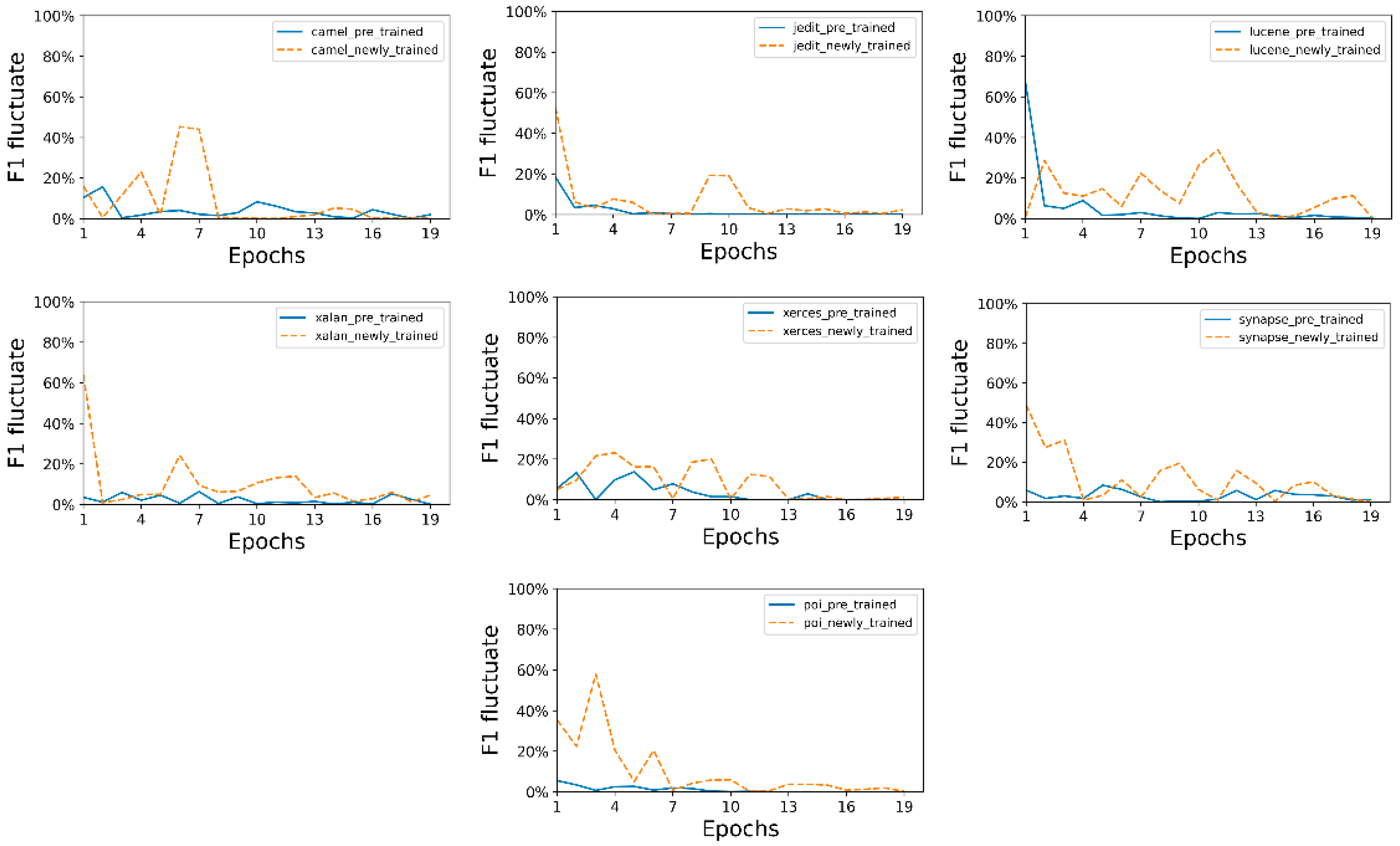
Apart from the prediction performance of the two models, the time cost of the two models also varies. We investigate the fluctuating level of F-measure on CodeBERT-NT and CodeBERT-PT for each project, as shown in
Figure 6. Despite the initial epochs, both models have good convergence. Specifically, the CodeBERT-PT model in solid blue line converges more quickly and has fewer fluctuations after several epochs, which shows less time cost. According to our statistics, training an effective CodeBERT-PT model could be four times faster than training an effective CodeBERT-NT model. This is easy to comprehend, as the CodeBERT-PT model is pre-trained by a large corpus. It greatly reduces the cost of learning syntactic and semantic rules of programming languages.
Summary of RQ1a: The prediction performance of CodeBERT-PT outperforms the CodeBERT-NT by 2.1% in cross-version software defect prediction. The CodeBERT-PT also trains four times faster than the CodeBERT-NT with lower fluctuations.
6.2.2. RQ1b: Does the Pre-Trained CodeBERT Model Outperform a Newly-Trained CodeBERT Model in Cross-Project Defect Prediction?
We perform cross-project experiments on the CPPSC dataset to compare the prediction performance of the CodeBERT-NT and CodeBERT-PT model on F-measure, as illustrated in
Table 4. For instance, we achieve an F-measure of 0.293 and 0.354 on the CodeBERT-NT and CodeBERT-PT model for the JEdit-Camel project. The RANDOM model achieves an F-measure of 0.255, which is lower than the CodeBERT-NT and CodeBERT-PT models. The CodeBERT-PT model outperforms the CodeBERT-NT model by 0.9% in terms of average F-measure. Both models also significantly outperform the RANDOM baseline at 0.402. Therefore, the CodeBERT-PT model outperforms the CodeBERT-NT model on the CVPSC dataset for cross-project defect prediction.
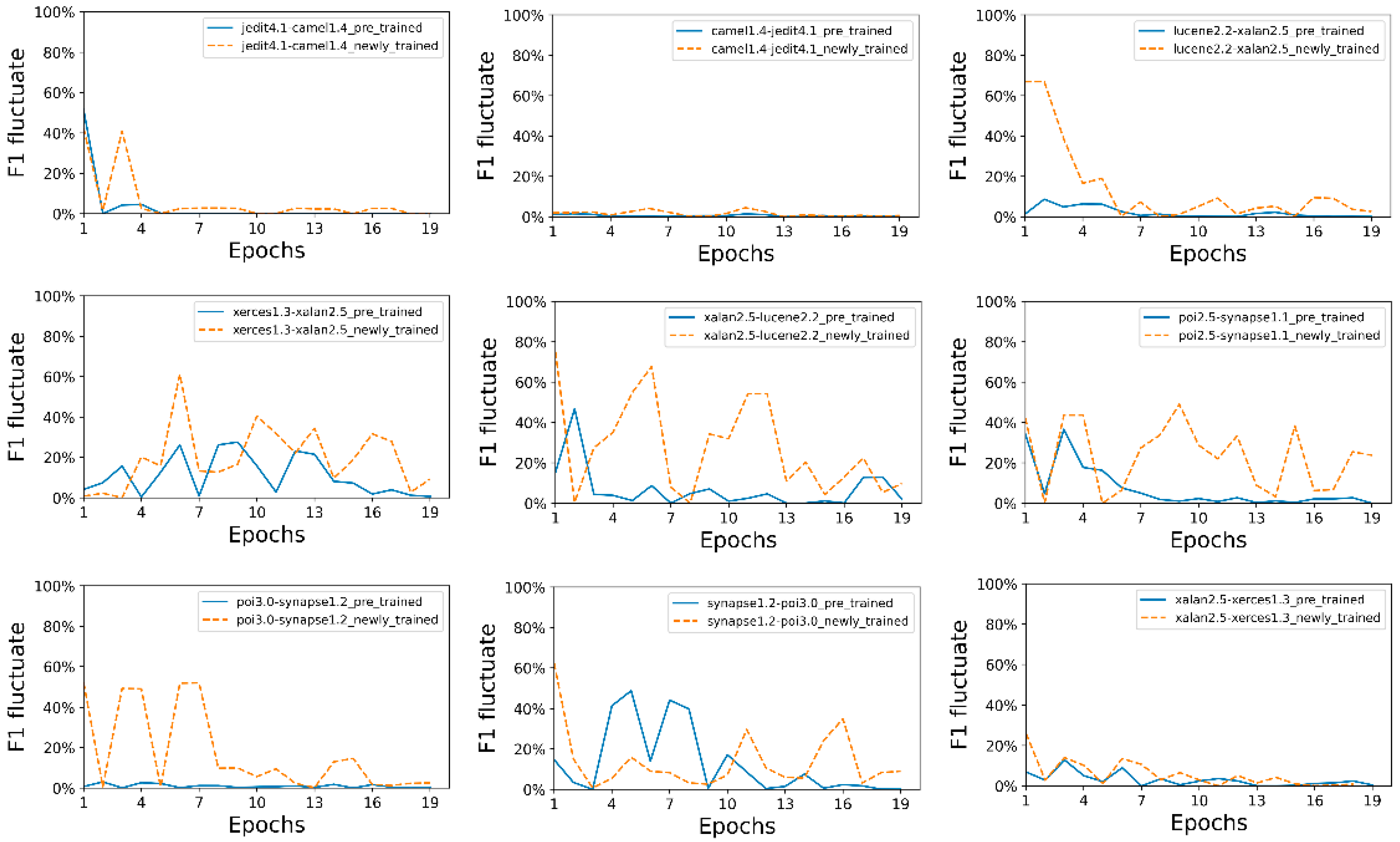
Apart from the prediction performance of the two models, the time cost of the two models also varies. We investigate the fluctuating level of F-measure on the CodeBERT-NT and CodeBERT-PT model for each project, as shown in
Figure 7. The
F1 level fluctuates more severely on the whole compared with
Figure 6 in RQ1a, indicating that the prediction performance of cross-project defect prediction is not as good as cross-version defect prediction, which is often the case in software defect prediction. Specifically, the CodeBERT-PT model in solid blue line converges more quickly and generally has fewer fluctuations, indicating less time cost. Statistics show that training a CodeBERT-PT model could be 1.5 times faster than training a CodeBERT-NT model. Although the CodeBERT-PT model also has advantages in time cost, the ratio decreases from 4 to 1.5 due to cross-project defect prediction.
Summary of RQ1b: The CodeBERT-PT outperforms the CodeBERT-NT model in cross-project software defect prediction. The CodeBERT-PT model also trains 1.5 times faster than the CodeBERT-NT model with lower fluctuations.
Summarizing RQ1a and RQ1b, we can conclude RQ1.
Summary of RQ1: The CodeBERT-PT model outperforms the CodeBERT-NT model in software defect prediction. The CodeBERT-PT model also trains much faster than the CodeBERT-NT model with lower fluctuations.
6.3. RQ2: Do the Different Prediction Patterns Affect Software Defect Prediction Performance?
We decompose RQ2 into two sub-research questions, RQ2a and RQ2b, that use the CVPSC and the CPPSC dataset for cross-version and cross-project defect prediction, perspectivity.
6.3.1. RQ2a: Do the Different Prediction Patterns Affect Software Defect Prediction Performance in Cross-Version Defect Prediction?
We perform cross-version defect prediction experiments on the CVPSC dataset to compare the prediction performance of CodeBERT-PS, CodeBERT-PK, and CodeBERT-PT model on F-measure, as illustrated in
Table 5. For instance, we achieve an F-measure of 0.505, 0.52, and 0.493 on the CodeBERT-PS, CodeBERT-PK, and CodeBERT-PT model for the Camel project. The RANDOM model for the Camel project achieves an F-measure of 0.287, which is lower than the three CodeBERT-based models. Considering the average F-measure, CodeBERT-PS and CodeBERT-PK models perform very similarly, which get 0.616 and 0.613, respectively. The CodeBERT-PT model performs poorer than the CodeBERT-PS and CodeBERT-PK models as a 5% decrease in F-measure. All three models outperform the RANDOM model, which achieves an F-measure of 0.397.
Summary of RQ2a: The CodeBERT-PS and CodeBERT-PK models behave similarly, and both outperform the CodeBERT-PT model in cross-version software defect prediction.
6.3.2. RQ2b: Do the Different Prediction Patterns Affect Software Defect Prediction Performance in Cross-Project Defect Prediction?
We perform cross-project defect prediction experiments on the CPPSC dataset to compare the prediction performance of CodeBERT-PS, CodeBERT-PK, CodeBERT-PT, and RANDOM models on F-measure, as illustrated in
Table 6. For instance, for the JEdit-Camel project, we achieve an F-measure of 0.357, 0.357, and 0.354 on the CodeBERT-PS, CodeBERT-PK, and CodeBERT-PT model. The RANDOM model achieves an F-measure of 0.255, which is lower than the three CodeBERT-based models. Considering the average F-measure, the CodeBERT-PS model outperforms the CodeBERT-PT models by 5% in F-measure, while the CodeBERT-PK model outperforms the CodeBERT-PT model by 3% in F-measure. All three models outperform the RANDOM model, which achieves an F-measure of 0.402.
Summary of RQ2b: The CodeBERT-PS and CodeBERT-PK models behave well, and both outperform the CodeBERT-PT model in cross-project software defect prediction. Specifically, the CodeBERT-PS model outperforms the CodeBERT-PK model.
Summarizing RQ2a and RQ2b, we can conclude RQ2.
Summary of RQ2: The CodeBERT-PS and CodeBERT-PK models behave well, and both outperform the CodeBERT-PT model in software defect prediction. Specifically, the CodeBERT-PS outperforms or at least is similar to the CodeBERT-PK model.
7. Discussion
7.1. Assumptions That Influence Software Defect Prediction
The empirical results of RQ1 indicate that using a pre-trained CodeBERT language model predicts defects more accurately and is more time-efficient than using a newly-trained model with the same architecture. The results of the time efficiency part are easy to understand, while the conclusions of the prediction performance part are more profounding. The result demonstrates that the naturalness assumption regarding software defect prediction can be proven by both statistics-based metrics like cross-entropy and deep learning models like neural language models. The advantage of neural language models over cross-entropy is that neural language models are more capable of characterizing the naturalness of code. The problem arises: How can the naturalness assumption be combined with other assumptions to enhance prediction performance?
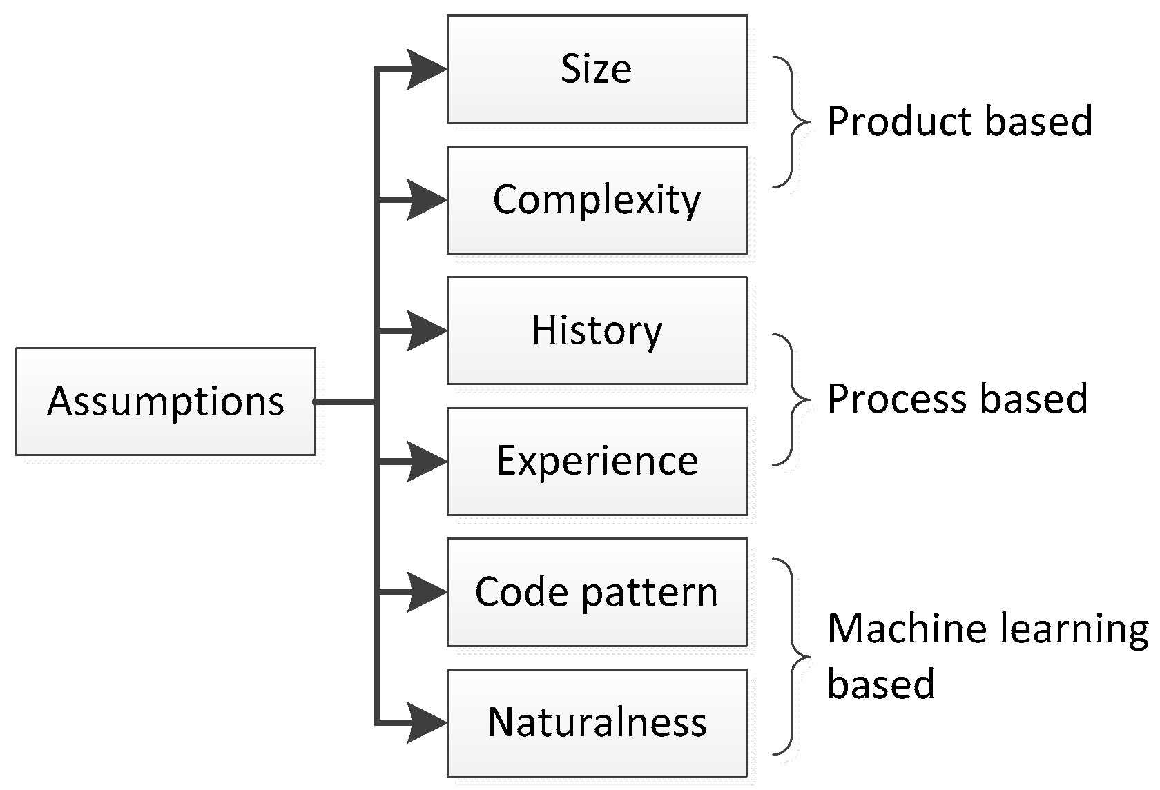
To solve the problem, we summarize and list the assumptions that influence software defect prediction in
Figure 8. The assumptions include:
- (1)
Product-based assumptions. Product-based assumptions focus on the scale and complexity of software. If the source code is large in size or complex, it is more likely to be buggy. Related metrics include LOC (lines of code) and CC (cyclomatic complexity) for source code, WMC (weighted method per class) and DIT (depth of inheritance) for object-oriented software, Degree and Betweenness Centrality for software complex networks.
- (2)
Process-based assumptions. Process-based assumptions focus on history and experience during the development process of software. If the historical version of the source code is buggy, or the source code is developed by inexperienced programmers, it is more likely to be buggy. Related metrics include code churn, fix, developer experience, developer interaction, ownership between software modules and developers, and so on.
- (3)
Machine learning-based assumptions. Machine learning-based assumptions focus on code patterns and naturalness. If the source code includes frequent patterns in buggy source code or the source code is unnatural, i.e., not following patterns followed by the majority of the developers, it is more likely to be buggy. Related metrics include semantic features generated from source code ASTs and neural language models.
As we use generated features for software defect prediction, and because the product-based and process-based features are mostly hand-crafted features, their combination does not seem to improve prediction performance that much. For example, Wang et al. [
4] tried to combine generated features and hand-crafted features and gain tiny improvements. Therefore, we infer that effective combinations of generated features should come from the machine learning-based assumption. Since the naturalness assumption has been proved in software defect prediction via neural language models, and the code pattern assumption has also been proven by various researchers in deep learning-based software defect prediction, it is worth investigating the relationship between the two assumptions. From our perspective, these two assumptions are demonstrated independently in the existing experimental design. For example, the use of AST nodes and AST paths proves that simplifying source code and highlighting components that are more related to defects can improve prediction performance in software defect prediction. The reason behind it may be that adding redundant information introduced by grammar definitions does not help improve prediction performance for software defect prediction. However, the CodeBERT model does not take advantage of ASTs and performs tokenization directly on the source code, which is generally accepted in text processing but can be improved in programming language processing. If a programming language model could be pre-trained using AST sequences or AST paths as input, it is more likely that the code pattern assumption and naturalness assumption can be combined in experimental design to further improve prediction performance.
7.2. The Relationship between Prediction Pattern and Buggy Rate
The empirical results of RQ2 indicate that CodeBERT-PK and CodeBERT-PS outperform CodeBERT-PT significantly. The key difference between them is the extra information from the keywords and sentences.
We investigate the relationship between keywords used in CodeBERT-PK and bug distribution, as shown in
Table 7. We first calculate the occurrences of keywords and exclude some unrelated cases that may confuse the statistics, e.g., “debug”, “prefix”, and “postfix”. We then count the number of samples that includes the keyword at least once and check whether it is a buggy sample or a clean sample. The buggy rate of samples that include the keywords is also calculated accordingly. The results show that the buggy rate of samples that include keywords is higher than the average buggy rate of 35.1%. The keyword-based prediction pattern highlights the relationship between the keywords and the prediction results, implying that source code that includes the keywords is more likely to be buggy. This may be the reason why CodeBERT-PK could outperform CodeBERT-PT in software defect prediction. The fact that the prediction performance of CodeBERT-PS outperforms or is similar to CodeBERT-PK indicates that the pre-trained CodeBERT model is capable of understanding natural language sentences that are strongly linked with the source code, which is proven in previous studies on the CodeBERT model. Specifically, the experimental settings of the CodeBERT-PS model could help in establishing implicit links among the purpose space (software defect prediction tasks), code semantic space (structural and semantics of the source code), and naturals text space (function names, variable names, etc.)
8. Threats to Validity
Programming language. Our dataset comes from the PROMISE repository, which is written in Java. However, our method is not limited to programming languages.
Dataset size. Our dataset uses a subset of the PROMISE repository, which is also used in previous work. Due to the limit that the project must be open-source, some datasets, i.e., the NASA dataset, are unavailable.
Selection of the CodeBERT model. We choose the standard CodeBERT model based on the RoBERTa architecture. Although other forms of CodeBERT models are available, e.g., graphCodeBERT, we believe the chosen model is powerful enough in our study.
9. Conclusions and Future Work
This paper proposes a variety of CodeBERT models targeting software defect prediction, including CodeBERT-NT, CodeBERT-PS, CodeBERT-PK, and CodeBERT-PT. We perform empirical studies using such models in cross-version and cross-project software defect prediction to investigate if using a neural language model like CodeBERT could improve prediction performance. We also investigate the effects of different prediction patterns in software defect prediction using CodeBERT models. The empirical results show that using a pre-trained CodeBERT model improves prediction performance and could save time cost. The empirical results also show that using sentence-based and keyword-based prediction patterns could improve the prediction performance of pre-trained neural language models for software defect prediction. We also discuss the assumptions that influence software defect prediction and the relationship between prediction patterns and buggy rate.
We would like to validate our results on AST node-based or AST path-based neural programming language models in the future. It is also interesting to investigate if the combination of comments as natural language texts and source code could further improve software defect prediction performance. It would also be of great value to replicate our findings in just-in-time software defect prediction using the latest datasets, e.g., the GHPR dataset [
50].
Author Contributions
Conceptualization, C.P.; methodology, C.P.; validation, C.P., B.X.; investigation, C.P.; data curation, C.P.; writing—original draft preparation, C.P.; writing—review and editing, M.L.; supervision, M.L. All authors have read and agreed to the published version of the manuscript.
Funding
This research received no external funding.
Data Availability Statement
Conflicts of Interest
The authors declare no conflict of interest.
References
- Menzies, T.; Milton, Z.; Turhan, B.; Cukic, B.; Jiang, Y.; Bener, A. Defect prediction from static code features: Current results, limitations, new approaches. Autom. Softw. Eng. 2010, 17, 375–407. [Google Scholar] [CrossRef]
- Krizhevsky, A.; Sutskever, I.; Hinton, G.E. Imagenet classification with deep convolutional neural networks. In Proceedings of the Advances in Neural Information Processing Systems, Lake Tahoe, NV, USA, 3–6 December 2012; pp. 1097–1105. [Google Scholar]
- Goodfellow, I.; Bengio, Y.; Courville, A. Deep learning. Nature 2015, 521, 436–444. [Google Scholar]
- Wang, S.; Liu, T.; Tan, L. Automatically learning semantic features for defect prediction. In Proceedings of the 2016 IEEE/ACM 38th International Conference on Software Engineering (ICSE), Austin, TX, USA, 14–22 May 2016; IEEE: New York, NY, USA, 2016; pp. 297–308. [Google Scholar]
- Li, J.; He, P.; Zhu, J.; Lyu, M.R. Software defect prediction via convolutional neural network. In Proceedings of the 2017 IEEE International Conference on Software Quality, Reliability and Security (QRS), Prague, Czech Republic, 25–29 July 2017; IEEE: New York, NY, USA, 2017; pp. 318–328. [Google Scholar]
- Deng, J.; Lu, L.; Qiu, S.; Ou, Y. A suitable ast node granularity and multi-kernel transfer convolutional neural network for cross-project defect prediction. IEEE Access 2020, 8, 66647–66661. [Google Scholar] [CrossRef]
- Pan, C.; Lu, M.; Xu, B.; Gao, H. An improved cnn model for within-project software defect prediction. Appl. Sci. 2019, 9, 2138. [Google Scholar] [CrossRef]
- Zhang, Q.; Wu, B. Software defect prediction via transformer. In Proceedings of the 2020 IEEE 4th Information Technology, Networking, Electronic and Automation Control Conference (ITNEC), Chongqing, China, 12–14 June 2020; IEEE: New York, NY, USA, 2020; Volume 1, pp. 874–879. [Google Scholar]
- Shi, K.; Lu, Y.; Chang, J.; Wei, Z. Pathpair2vec: An ast path pair-based code representation method for defect prediction. J. Comput. Lang. 2020, 59, 100979. [Google Scholar] [CrossRef]
- Hoang, T.; Dam, H.K.; Kamei, Y.; Lo, D.; Ubayashi, N. Deepjit: An end-to-end deep learning framework for just-in-time defect prediction. In Proceedings of the 2019 IEEE/ACM 16th International Conference on Mining Software Repositories (MSR), Montreal, QC, Canada, 25–31 May 2019; IEEE: New York, NY, USA, 2019; pp. 34–45. [Google Scholar]
- Chen, D.; Chen, X.; Li, H.; Xie, J.; Mu, Y. Deepcpdp: Deep learning based cross-project defect prediction. IEEE Access 2019, 7, 184832–184848. [Google Scholar] [CrossRef]
- Liang, H.; Yu, Y.; Jiang, L.; Xie, Z. Seml: A semantic lstm model for software defect prediction. IEEE Access 2019, 7, 83812–83824. [Google Scholar] [CrossRef]
- Qiao, L.; Li, X.; Umer, Q.; Guo, P. Deep learning based software defect prediction. Neurocomputing 2020, 385, 100–110. [Google Scholar] [CrossRef]
- Majd, A.; Vahidi-Asl, M.; Khalilian, A.; Poorsarvi-Tehrani, P.; Haghighi, H. SLDeep: Statement-level software defect prediction using deep-learning model on static code features. Expert Syst. Appl. 2020, 147, 113156. [Google Scholar] [CrossRef]
- Hasanpour, A.; Farzi, P.; Tehrani, A.; Akbari, R. Software Defect Prediction Based on Deep Learning Models: Performance Study. arXiv 2020, arXiv:2004.02589. [Google Scholar]
- Deng, J.; Lu, L.; Qiu, S. Software defect prediction via LSTM. IET Softw. 2020, 14, 443–450. [Google Scholar] [CrossRef]
- Shi, K.; Lu, Y.; Liu, G.; Wei, Z.; Chang, J. MPT-embedding: An unsupervised representation learning of code for software defect prediction. J. Softw. Evol. Proc. 2020, 33, e2330. [Google Scholar]
- Lin, J.; Lu, L. Semantic Feature Learning via Dual Sequences for Defect Prediction. IEEE Access 2021, 9, 13112–13124. [Google Scholar] [CrossRef]
- Meilong, S.; He, P.; Xiao, H.; Li, H.; Zeng, C. An Approach to Semantic and Structural Features Learning for Software Defect Prediction. Math. Probl. Eng. 2020, 1–13. [Google Scholar] [CrossRef]
- Omri, S.; Sinz, C. Deep Learning for Software Defect Prediction: A Survey. In Proceedings of the IEEE/ACM 42nd International Conference on Software Engineering Workshops, Seoul, Korea, 16–24 June 2020; pp. 209–214. [Google Scholar]
- Tian, J.; Tian, Y. A Model Based on Program Slice and Deep Learning for Software Defect Prediction. In Proceedings of the 2020 29th International Conference on Computer Communications and Networks (ICCCN), Honolulu, HI, USA, 3–6 August 2020; IEEE: New York, NY, USA, 2020; pp. 1–6. [Google Scholar]
- Lin, X.; Yang, J.; Li, Z. Software Defect Prediction with Spiking Neural Networks. In Proceedings of the International Conference on Neural Information Processing, Bangkok, Thailand, 18–22 November 2020; Springer: Berlin/Heidelberg, Germany, 2020; pp. 660–667. [Google Scholar]
- Zhu, K.; Zhang, N.; Zhang, Q.; Ying, S.; Wang, X. Software defect prediction based on non-linear manifold learning and hybrid deep learning techniques. Comput. Mater. Contin. 2020, 65, 1467–1486. [Google Scholar] [CrossRef]
- Wongpheng, K.; Visutsak, P. Software Defect Prediction using Convolutional Neural Network. In Proceedings of the 2020 35th International Technical Conference on Circuits/Systems, Computers and Communications (ITC-CSCC), Nagoya, Japan, 3–6 July 2020; IEEE: New York, NY, USA, 2020; pp. 240–243. [Google Scholar]
- Sheng, L.; Lu, L.; Lin, J. An adversarial discriminative convolutional neural network for cross-project defect prediction. IEEE Access 2020, 8, 55241–55253. [Google Scholar] [CrossRef]
- Mikolov, T.; Chen, K.; Corrado, G.; Dean, J. Efficient Estimation of Word Representations in Vector Space. arXiv 2013, arXiv:1301.3781. [Google Scholar]
- Pennington, J.; Socher, R.; Manning, C.D. Glove: Global vectors for word representation. In Proceedings of the 2014 Conference on Empirical Methods in Natural Language Processing (EMNLP), Doha, Qatar, 25–29 October 2014; pp. 1532–1543. [Google Scholar]
- Devlin, J.; Chang, M.W.; Lee, K.; Toutanova, K. Bert: Pre-training of deep bidirectional transformers for language understanding. arXiv 2018, arXiv:1810.04805. [Google Scholar]
- Allamanis, M.; Barr, E.T.; Bird, C.; Sutton, C. Suggesting accurate method and class names. In Proceedings of the 2015 10th Joint Meeting on Foundations of Software Engineering, ESEC/FSE 2015, Bergamo, Italy, 30 August–4 September 2015; ACM: New York, NY, USA, 2015; pp. 38–49. [Google Scholar]
- Mou, L.; Li, G.; Zhang, L.; Wang, T.; Jin, Z. Convolutional neural networks over tree structures for programming language processing. In Proceedings of the Thirtieth AAAI Conference on Artificial Intelligence, AAAI’16, Phoenix, AZ, USA, 12–17 February 2016; AAAI Press: Palo Alto, CA, USA, 2016; pp. 1287–1293. [Google Scholar]
- Zhang, J.; Wang, X.; Zhang, H.; Sun, H.; Wang, K.; Liu, X. A novel neural source code representation based on abstract syntax tree. In Proceedings of the 2019 IEEE/ACM 41st International Conference on Software Engineering (ICSE), Montreal, QC, Canada, 25–31 May 2019; IEEE: New York, NY, USA, 2019; pp. 783–794. [Google Scholar]
- Alon, U.; Zilberstein, M.; Levy, O.; Yahav, E. Code2vec: Learning distributed representations of code. Proc. ACM Program Lang. 3(POPL) 2019, 40, 1–29. [Google Scholar] [CrossRef]
- Li, Y.; Tarlow, D.; Brockschmidt, M.; Zemel, R.S. Gated graph sequence neural networks. In Proceedings of the 4th International Conference on Learning Representations, ICLR 2016, San Juan, Puerto Rico, 2–4 May 2016. [Google Scholar]
- Allamanis, M. The adverse effects of code duplication in machine learning models of code. In Proceedings of the 2019 ACM SIGPLAN International Symposium on New Ideas, New Paradigms, and Reflections on Programming and Software; Association for Computing Machinery: New York, NY, USA, 2019; pp. 143–153. [Google Scholar]
- Hellendoorn, V.J.; Sutton, C.; Singh, R.; Maniatis, P.; Bieber, D. Global relational models of source code. In Proceedings of the International Conference on Learning Representations, Addis Ababa, Ethiopia, 26–30 April 2020. [Google Scholar]
- Feng, Z.; Guo, D.; Tang, D.; Duan, N.; Feng, X.; Gong, M.; Shou, L.; Qin, B.; Liu, T.; Jiang, D.; et al. CodeBERT: A pre-trained model for programming and natural languages. arXiv 2020, arXiv:2002.08155. [Google Scholar]
- Yang, X.; Lo, D.; Xia, X.; Zhang, Y.; Sun, J. Deep learning for just-in-time defect prediction. In Proceedings of the 2015 IEEE International Conference on Software Quality, Reliability and Security, Vancouver, BC, Canada, 3–5 August 2015; IEEE: New York, NY, USA, 2015; pp. 17–26. [Google Scholar]
- Tong, H.; Liu, B.; Wang, S. Software defect prediction using stacked denoising autoencoders and two-stage ensemble learning. Inf. Softw. Technol. 2018, 96, 94–111. [Google Scholar] [CrossRef]
- Sun, J.; Ji, Y.; Liu, S.; Wu, F. Cost-Sensitive and Sparse Ladder Network for Software Defect Prediction. IEICE Trans. Inf. Syst. 2020, 103, 1177–1180. [Google Scholar] [CrossRef]
- Torrey, L.; Shavlik, J. Transfer learning. In Handbook of Research on Machine Learning Applications and Trends: Algorithms, Methods, and Techniques; IGI Global: Hershey, PA, USA, 2010; pp. 242–264. [Google Scholar]
- Tan, C.; Sun, F.; Kong, T.; Zhang, W.; Yang, C.; Liu, C. A survey on deep transfer learning. In Proceedings of the International Conference on Artificial Neural Networks, Rhodes, Greece, 4–7 October 2018; Springer: Berlin/Heidelberg, Germany, 2018; pp. 270–279. [Google Scholar]
- Brown, T.B.; Mann, B.; Ryder, N.; Subbiah, M.; Kaplan, J.; Dhariwal, P.; Neelakantan, A.; Shyam, P.; Sastry, G.; Askell, A.; et al. Language models are few-shot learners. arXiv 2020, arXiv:2005.14165. [Google Scholar]
- Liu, Y.; Ott, M.; Goyal, N.; Du, J.; Joshi, M.; Chen, D.; Levy, O.; Lewis, M.; Zettlemoyer, L.; Stoyanov, V. Roberta: A robustly optimized bert pretraining approach. arXiv 2019, arXiv:1907.11692. [Google Scholar]
- Vaswani, A.; Shazeer, N.; Parmar, N.; Uszkoreit, J.; Jones, L.; Gomez, A.N.; Kaiser, L.; Polosukhin, I. Attention is all you need. arXiv 2017, arXiv:1706.03762. [Google Scholar]
- Raym, B.; Hellendoorn, V.; Godhane, S.; Tu, Z.; Bacchelli, A.; Devanbu, P. On the “naturalness” of buggy code. In Proceedings of the 2016 IEEE/ACM 38th International Conference on Software Engineering (ICSE), Austin, TX, USA, 14–22 May 2016; IEEE: New York, NY, USA, 2016; pp. 428–439. [Google Scholar]
- Allamanis, M.; Barr, E.T.; Devanbu, P.; Sutton, C. A survey of machine learning for big code and naturalness. ACM Comput. Surv. 2018, 51, 1–37. [Google Scholar] [CrossRef]
- Buratti, L.; Pujar, S.; Bornea, M.; McCarley, S.; Zheng, Y.; Rossiello, G.; Domeniconi, G. Exploring Software Naturalness through Neural Language Models. arXiv 2020, arXiv:2006.12641. [Google Scholar]
- CodeBERT on HuggingFace. Available online: https://huggingface.co/microsoft/codebert-base (accessed on 22 March 2021).
- Jureczko, M.; Madeyski, L. Towards identifying software project clusters with regard to defect prediction. In Proceedings of the 6th International Conference on Predictive, Jinan, China, 18–20 September 2010. [Google Scholar]
- Xu, J.; Yan, L.; Wang, F.; Ai, J. A GitHub-Based Data Collection Method for Software Defect Prediction. In Proceedings of the 2019 6th International Conference on Dependable Systems and Their Applications (DSA), Harbin, China, 3–6 January 2020; IEEE: New York, NY, USA, 2020; pp. 100–108. [Google Scholar]
Figure 1.
Workflow of deep learning based software defect prediction.
Figure 1.
Workflow of deep learning based software defect prediction.
Figure 2.
A typical process of network-based deep transfer learning.
Figure 2.
A typical process of network-based deep transfer learning.
Figure 3.
The overall architecture of BERT.
Figure 3.
The overall architecture of BERT.
Figure 4.
The overall workflow of our approach for software defect prediction.
Figure 4.
The overall workflow of our approach for software defect prediction.
Figure 5.
Traditional, sentence-based, and keyword-based prediction patterns. The classification model is omitted for simplicity.
Figure 5.
Traditional, sentence-based, and keyword-based prediction patterns. The classification model is omitted for simplicity.
Figure 6.
The fluctuating level of F-measure on CodeBERT-PT and CodeBERT-NT on the CVPSC dataset for cross-version defect prediction.
Figure 6.
The fluctuating level of F-measure on CodeBERT-PT and CodeBERT-NT on the CVPSC dataset for cross-version defect prediction.
Figure 7.
The fluctuating level of F-measure on CodeBERT-PT and CodeBERT-NT on the CPPSC dataset for cross-project defect prediction.
Figure 7.
The fluctuating level of F-measure on CodeBERT-PT and CodeBERT-NT on the CPPSC dataset for cross-project defect prediction.
Figure 8.
Assumptions that influence software defect prediction.
Figure 8.
Assumptions that influence software defect prediction.
Table 1.
CVPSC dataset description. The number of files, number of defects, and average buggy rate are listed separately for the training set and the test set.
Table 1.
CVPSC dataset description. The number of files, number of defects, and average buggy rate are listed separately for the training set and the test set.
| Training Set | Test Set | No. Files | No. Defects | Avg. Buggy Rate |
|---|
| Camel 1.4 | Camel 1.6 | 847/934 | 145/188 | 17.1%/20.1% |
| JEdit 4.0 | JEdit 4.1 | 184/367 | 67/67 | 36.4%/18.3% |
| Lucene 2.0 | Lucene 2.2 | 186/238 | 91/143 | 48.9%/60.1% |
| Xalan 2.5 | Xalan 2.6 | 755/877 | 380/411 | 50.3%/46.9% |
| Xerces 1.2 | Xerces 1.3 | 436/446 | 70/67 | 16.1%/15% |
| Synapse 1.1 | Synapse 1.2 | 205/256 | 55/86 | 26.8%/33.6% |
| Poi 2.5 | Poi 3.0 | 380/438 | 248/281 | 65.3%/64.2% |
| Total | 6549 | 2299 | 35.1% |
Table 2.
CPPSC dataset description. The number of files, number of defects, and average buggy rate are listed separately for the training set and the test set.
Table 2.
CPPSC dataset description. The number of files, number of defects, and average buggy rate are listed separately for the training set and the test set.
| Training Set | Test Set | No. Files | No. Defects | Avg. Buggy Rate |
|---|
| JEdit 4.1 | Camel 1.4 | 367/847 | 67/145 | 18.3%/17.1% |
| Camel 1.4 | JEdit 4.1 | 847/367 | 145/67 | 17.1%/18.3% |
| Lucene 2.2 | Xalan 2.5 | 238/755 | 143/380 | 48.9%/50.3% |
| Xerces 1.3 | Xalan 2.5 | 446/755 | 67/380 | 15%/50.3% |
| Xalan 2.5 | Lucene 2.2 | 755/238 | 380/143 | 50.3%/48.9% |
| Poi 2.5 | Synapse 1.1 | 380/205 | 248/55 | 65.3%/26.8% |
| Poi 3.0 | Synapse 1.2 | 438/256 | 281/86 | 64.2/33.6% |
| Synapse 1.2 | Poi 3.0 | 256/438 | 86/281 | 33.6%/64.2% |
| Xalan 2.5 | Xerces 1.3 | 755/446 | 380/67 | 50.3%/15% |
| Total | 8589 | 3401 | 39.6% |
Table 3.
Performance comparison of CodeBERT-NT, CodeBERT-PT, and RANDOM models on the CVPSC dataset for cross-version defect prediction. The float values are the average F-measure values. The best F-measure values are highlighted in bold.
Table 3.
Performance comparison of CodeBERT-NT, CodeBERT-PT, and RANDOM models on the CVPSC dataset for cross-version defect prediction. The float values are the average F-measure values. The best F-measure values are highlighted in bold.
| Training Set | Test Set | CodeBERT-NT | CodeBERT-PT | RANDOM |
|---|
| Camel 1.4 | Camel 1.6 | 0.509 | 0.493 | 0.287 |
| JEdit 4.0 | JEdit 4.1 | 0.567 | 0.642 | 0.267 |
| Lucene 2.0 | Lucene 2.2 | 0.653 | 0.707 | 0.546 |
| Xalan 2.5 | Xalan 2.6 | 0.581 | 0.627 | 0.484 |
| Xerces 1.2 | Xerces 1.3 | 0.349 | 0.321 | 0.231 |
| Synapse 1.1 | Synapse 1.2 | 0.445 | 0.443 | 0.402 |
| Poi 2.5 | Poi 3.0 | 0.702 | 0.72 | 0.562 |
| Average | 0.544 | 0.565 | 0.397 |
Table 4.
Performance comparison of CodeBERT-NT, CodeBERT-PT, and RANDOM models on the CPPSC dataset for cross-project defect prediction. The float values are the average F-measure values. The best F-measure values are highlighted in bold.
Table 4.
Performance comparison of CodeBERT-NT, CodeBERT-PT, and RANDOM models on the CPPSC dataset for cross-project defect prediction. The float values are the average F-measure values. The best F-measure values are highlighted in bold.
| Training Set | Test Set | CodeBERT-NT | CodeBERT-PT | RANDOM |
|---|
| JEdit 4.1 | Camel 1.4 | 0.293 | 0.354 | 0.255 |
| Camel 1.4 | JEdit 4.1 | 0.342 | 0.36 | 0.267 |
| Lucene 2.2 | Xalan 2.5 | 0.707 | 0.66 | 0.502 |
| Xerces 1.3 | Xalan 2.5 | 0.627 | 0.659 | 0.502 |
| Xalan 2.5 | Lucene 2.2 | 0.321 | 0.648 | 0.546 |
| Poi 2.5 | Synapse 1.1 | 0.443 | 0.431 | 0.349 |
| Poi 3.0 | Synapse 1.2 | 0.72 | 0.531 | 0.402 |
| Synapse 1.2 | Poi 3.0 | 0.493 | 0.587 | 0.562 |
| Xalan 2.5 | Xerces 1.3 | 0.642 | 0.445 | 0.231 |
| Average | 0.51 | 0.519 | 0.402 |
Table 5.
Performance comparison of CodeBERT-PS, CodeBERT-PK, CodeBERT-PT, and RANDOM models on the CVPSC dataset for cross-version defect prediction. The float values are the average F-measure values. The best F-measure values are highlighted in bold.
Table 5.
Performance comparison of CodeBERT-PS, CodeBERT-PK, CodeBERT-PT, and RANDOM models on the CVPSC dataset for cross-version defect prediction. The float values are the average F-measure values. The best F-measure values are highlighted in bold.
| Training Set | Test Set | CodeBERT-PS | CodeBERT-PK | CodeBERT-PT | RANDOM |
|---|
| Camel 1.4 | Camel 1.6 | 0.505 | 0.52 | 0.493 | 0.287 |
| JEdit 4.0 | JEdit 4.1 | 0.661 | 0.701 | 0.642 | 0.267 |
| Lucene 2.0 | Lucene 2.2 | 0.743 | 0.741 | 0.707 | 0.546 |
| Xalan 2.5 | Xalan 2.6 | 0.684 | 0.675 | 0.627 | 0.484 |
| Xerces 1.2 | Xerces 1.3 | 0.36 | 0.313 | 0.321 | 0.231 |
| Synapse 1.1 | Synapse 1.2 | 0.566 | 0.548 | 0.443 | 0.402 |
| Poi 2.5 | Poi 3.0 | 0.795 | 0.795 | 0.72 | 0.562 |
| Average | 0.616 | 0.613 | 0.565 | 0.397 |
Table 6.
Performance comparison of CodeBERT-PS, CodeBERT-PK, CodeBERT-PT, and RANDOM models on the CPPSC dataset for cross-project defect prediction. The float values are the average F-measure values. The best F-measure values are highlighted in bold.
Table 6.
Performance comparison of CodeBERT-PS, CodeBERT-PK, CodeBERT-PT, and RANDOM models on the CPPSC dataset for cross-project defect prediction. The float values are the average F-measure values. The best F-measure values are highlighted in bold.
| Training Set | Test Set | CodeBERT-PS | CodeBERT-PK | CodeBERT-PT | RANDOM |
|---|
| JEdit 4.1 | Camel 1.4 | 0.357 | 0.357 | 0.354 | 0.255 |
| Camel 1.4 | JEdit 4.1 | 0.543 | 0.556 | 0.36 | 0.267 |
| Lucene 2.2 | Xalan 2.5 | 0.672 | 0.662 | 0.66 | 0.502 |
| Xerces 1.3 | Xalan 2.5 | 0.651 | 0.65 | 0.659 | 0.502 |
| Xalan 2.5 | Lucene 2.2 | 0.745 | 0.714 | 0.648 | 0.546 |
| Poi 2.5 | Synapse 1.1 | 0.482 | 0.516 | 0.431 | 0.349 |
| Poi 3.0 | Synapse 1.2 | 0.533 | 0.545 | 0.531 | 0.402 |
| Synapse 1.2 | Poi 3.0 | 0.682 | 0.568 | 0.587 | 0.562 |
| Xalan 2.5 | Xerces 1.3 | 0.463 | 0.392 | 0.445 | 0.231 |
| Average | 0.57 | 0.551 | 0.519 | 0.402 |
Table 7.
Relationship between keywords used in CodeBERT-PK and buggy rate.
Table 7.
Relationship between keywords used in CodeBERT-PK and buggy rate.
| Keyword | Count | No. Samples | No. Defects | No. Non-Defects | Buggy Rate |
|---|
| Bug | 24 | 8 | 4 | 4 | 50% |
| Defect | 14 | 4 | 3 | 1 | 75% |
| Fail | 302 | 120 | 47 | 73 | 39.2% |
| Error | 3011 | 654 | 326 | 328 | 49.8% |
| Patch | 562 | 93 | 55 | 38 | 59.1% |
| Publisher’s Note: MDPI stays neutral with regard to jurisdictional claims in published maps and institutional affiliations. |
© 2021 by the authors. Licensee MDPI, Basel, Switzerland. This article is an open access article distributed under the terms and conditions of the Creative Commons Attribution (CC BY) license (https://creativecommons.org/licenses/by/4.0/).


