Neural Network Control for Trajectory Tracking and Balancing of a Ball-Balancing Robot with Uncertainty

Abstract

In this paper, a neural-network-based control method to achieve trajectory tracking and balancing of a ball-balancing robot with uncertainty is presented. Because the ball-balancing robot is an underactuated system and has nonlinear couplings in the dynamic model, it is challenging to design a controller for trajectory tracking and balancing. Thus, various approaches have been proposed to solve these problems. However, there are still problems such as the complex control system and instability. Therefore, the objective of this paper was to propose a solution to these problems. To this end, we developed a virtual angle-based control scheme. Because the virtual angle was used as the reference angle to achieve trajectory tracking while keeping the balance of the ball-balancing robot, we could solve the underactuation problem using a single-loop controller. The radial basis function networks (RBFNs) were employed to compensate uncertainties, and the controller was designed using the dynamic surface control (DSC) method. From the Lyapunov stability theory, it was proven that all errors of the closed-loop control system were uniformly ultimately bounded. Therefore, the control system structure was simple and ensured stability in achieving simultaneous trajectory tracking and balancing of the ball-balancing robot with uncertainty. Finally, the simulation results are given to verify the performance of the proposed controller through comparison results. As a result, the proposed method showed a $19.2\%$ improved tracking error rate compared to the existing method.

1. Introduction

Mobile robots have been attracting attention in many fields due to their various applications. Therefore, various techniques have been proposed to operate mobile robots, such as automatic control and a brain–computer interface (BCI) that connects the brain and a computer to control the robot [1]. In this paper, we focused on the automatic control of a ball-balancing robot, which is a type of mobile robot. The ball-balancing robot is an omnidirectional mobile robot, the body of which is placed over a spherical wheel. Because of this characteristic, a control strategy different from traditional methods for mobile robots was required to achieve simultaneous trajectory tracking and balancing. However, designing the controller was challenging due to several problems such as underactuation and nonlinear coupling.

Early studies used single-loop control methods such as proportional–integral–derivative (PID) [2] and a linear quadratic regulator (LQR) [3], which was only possible for balancing the robot. To enable both trajectory tracking and balancing of the robot, multi-loop control methods such as PI-LQR [4] and PD-PID [5] were presented using independent inner- and outer-loops. However, the above papers were based on the linearized model, which requires a narrow operating range. Although the partial feedback linearization (PFL) technique [6] was proposed to relax this restriction, the control system using the multi-loop method becomes complex due to additional feed-forward controllers for robustness against uncertainties [7].

Sliding mode control (SMC) is a representative nonlinear control method that is robust to uncertainty. Thus, the hierarchical sliding mode control (HSMC) method [8], which is composed of combinations of independent sliding surfaces, was proposed to address underactuated systems. The HSMC method based on the two-dimensional model of the ball-balancing robot was presented in [9] and then applied to the aggregated model to consider the combined effects [10]. An integral backstepping technique using the HSMC structure was proposed in [11], and an artificial neural network-based method [12] was presented to deal with uncertainty and input saturation. The hierarchical structure used in the above papers can solve the underactuation problem and has robustness for uncertainties. However, the hierarchical structure has the local minimum problem [13], which may not guarantee the convergence of all errors.

Therefore, a different approach was needed to achieve simultaneous trajectory tracking and balancing for the ball-balancing robot. In this regard, we proposed a virtual angle-based approach [14]. The virtual angle composed of the tracking errors was used as a reference angle to achieve simultaneous trajectory tracking and balancing using the single-loop control system. However, the upper bounds of uncertainties for robustness should be known, which may be impossible in the real world. Artificial intelligence can be a solution to address this problem. In [15], deterministic artificial intelligence (DAI) was used for underactuated systems with nonlinear couplings. In [16], a artificial neural network was employed to deal with model uncertainty and the external disturbance of underactuated surface vessels. The field of non-stochastic or DAI involves the assertion of self-awareness statements and uses optimal learning to compensate the deleterious effects of error sources [15]. On the other hand, an artificial neural network (ANN), which is in the field of stochastic artificial intelligence, does not need to devise an algorithm to perform a particular task because the learning process of a neural network takes place by itself [17].

Motivated by these observations, we proposed a neural network-based control for trajectory tracking and balancing of the ball-balancing robot with uncertainty. A virtual angle-based control method was used to design a single-loop control system to achieve trajectory tracking and balancing of the robot. Unlike in [14], the radial basis function networks (RBFNs) [18], a kind of ANN, were used to compensate the uncertainties without knowing their upper bounds, and the dynamic surface control (DSC) method [19] was employed to design the controller. From the Lyapunov stability theory, it was proven that all errors of the closed-loop control system were uniformly ultimately bounded. Finally, the performance of the proposed method was demonstrated through the simulation results.

The main contributions of this paper are summarized as follows:

• The trajectory tracking and balancing of the ball-balancing robot was achieved using a single-loop controller;
• It was possible to implement a control system without any knowledge of the upper bounds of uncertainties.

This paper is organized as follows. In Section 2, the dynamics of the ball-balancing robot and the RBFNs are described, and the neural network-based controller is developed for trajectory tracking and balancing of the ball-balancing robot. In Section 3, the simulation results are presented to demonstrate the performance of the proposed method, and the discussion is given in Section 4.

2. Materials and Methods

In this section, we describe the system model of the ball-balancing robot for formulating the problems and introduce the RBFNs for compensating the uncertainty.

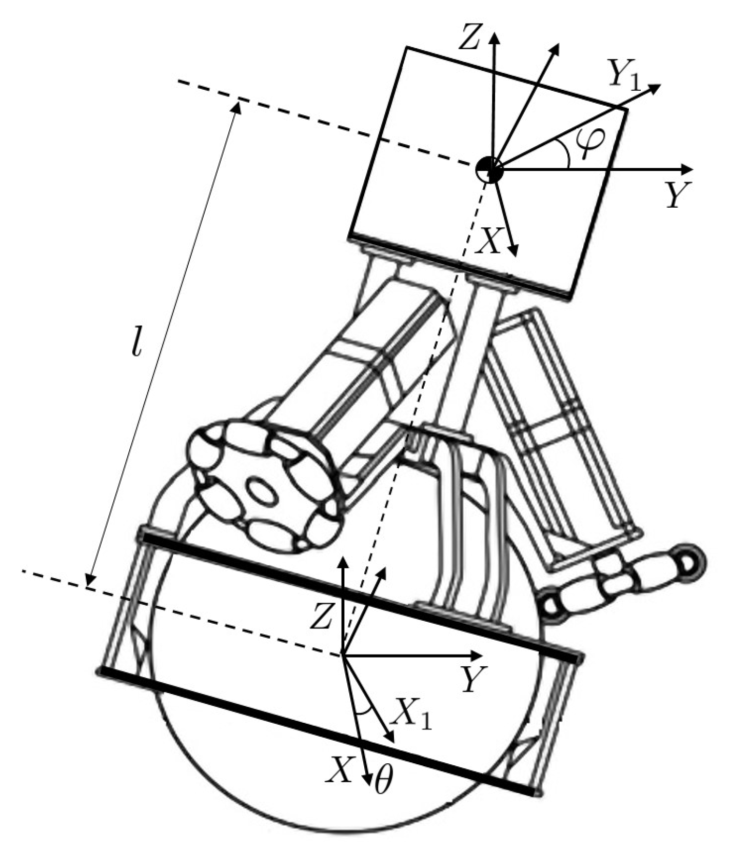
2.1. Dynamics of the Ball-Balancing Robot

Consider the ball-balancing robot shown in Figure 1. Assuming that there is no slip between the sphere and the floor and between the driving wheels and the sphere, the dynamic equation of the ball-balancing robot can be expressed as [12]:

$$\begin{array}{c}\hfill \mathit{M}\left(\mathit{q}\right)\ddot{\mathit{q}}+\mathit{C}(\dot{\mathit{q}},\mathit{q})\dot{\mathit{q}}+\mathit{f}\left(\dot{\mathit{q}}\right)+\mathit{g}\left(\mathit{q}\right)=\mathit{B}\left(\mathit{q}\right)\mathit{u}.\end{array}$$

(1)

Here, $\mathit{M}\left(\mathit{q}\right)\in {\mathbb{R}}^{4\times 4}$ is the symmetric inertia matrix, $\mathit{C}(\dot{\mathit{q}},\mathit{q})\in {\mathbb{R}}^{4\times 4}$ represents the Coriolis and centripetal matrix, $\mathit{f}\left(\dot{\mathit{q}}\right)\in {\mathbb{R}}^4$ is the friction matrix, $\mathit{g}\left(\mathit{q}\right)\in {\mathbb{R}}^4$ is the gravity vector, $\mathit{B}\left(\mathit{q}\right)\in {\mathbb{R}}^{4\times 2}$ denotes control input matrix, and $\mathit{u}\in {\mathbb{R}}^2$ represents the control input vector. These terms are given by:

$$\begin{array}{cc}\hfill & \mathit{M}\left(\mathit{q}\right)=\left[\begin{array}{cccc}{m}_1& m_2& m_3& m_4\\ m_2& m_5& m_6& m_7\\ m_3& m_6& m_8& 0\\ m_4& m_7& 0& m_9\end{array}\right],\hfill \\ \hfill & \mathit{C}(\dot{\mathit{q}},\mathit{q})=\left[\begin{array}{cccc}{c}_{11}& c_{12}& c_{13}& c_{14}\\ c_{21}& c_{22}& c_{23}& c_{24}\\ c_{31}& c_{32}& c_{33}& c_{34}\\ c_{41}& c_{42}& 0& c_{44}\end{array}\right],\hfill \\ \hfill & \mathit{f}\left(\dot{\mathit{q}}\right)={\left[\begin{array}{c}{\zeta }_x\dot{x},{\zeta }_y\dot{y},{\zeta }_{\theta }\dot{\theta },{\zeta }_{\phi }\dot{\phi }\end{array}\right]}^{\top },\hfill \\ \hfill & \mathit{g}\left(\mathit{q}\right)={\left[\begin{array}{c}0,0,g_3,g_4\end{array}\right]}^{\top },\mathit{u}={\left[\begin{array}{c}{u}_x,u_y\end{array}\right]}^{\top },\hfill \\ \hfill & \mathit{B}\left(\mathit{q}\right)={\left[\begin{array}{c}{\mathit{B}}_s^{\top },{\mathit{B}}_b^{\top }\end{array}\right]}^{\top },\mathit{q}={\left[\begin{array}{c}x,y,\theta ,\phi \end{array}\right]}^{\top },\hfill \\ \hfill & {\mathit{B}}_s=\frac{1}{r_w}{\left[\begin{array}{cc}0& -cos\phi \\ cos\theta & sin\phi cos\theta \end{array}\right]}^{\top },{\mathit{B}}_b=\frac{r_s}{r_w}{\left[\begin{array}{cc}0& 1\\ 1& 0\end{array}\right]}^{\top },\hfill \end{array}$$

where the X- and Y-axis positions of the ball are denoted by x and y, respectively, pitch and roll are denoted by $\theta$ and $\phi$, respectively, and $u_x$ and $u_y$ denote the control inputs of the virtual acting wheels by the three omnidirectional wheels, respectively. The terms in ${\zeta }_i(i=x,y,\theta ,\phi )$ are viscous coefficients. $r_s$ and $r_w$ denote the ball radius and omnidirectional wheel radius, respectively. It is noted that control input matrices ${\mathit{B}}_s$ and ${\mathit{B}}_b$ are invertible with $\left|\theta \right|$, $\left|\phi \right|$$<\pi /2$. The terms in $\mathit{M}\left(\mathit{q}\right)$, $\mathit{C}(\dot{\mathit{q}},\mathit{q})$, and $\mathit{g}\left(\mathit{q}\right)$ are given in Appendix A.

The dynamic equation in (1) can be decoupled into two subsystems of the position and the angle as follows:

$$\begin{array}{cc}\hfill & {\ddot{\mathit{q}}}_s={\mathit{F}}_s+\Delta {\mathit{F}}_s+{\mathit{G}}_s\mathit{u},\hfill \end{array}$$

(2)

$$\begin{array}{cc}\hfill & {\ddot{\mathit{q}}}_b={\mathit{F}}_b+\Delta {\mathit{F}}_b+{\mathit{G}}_b\mathit{u}.\hfill \end{array}$$

(3)

In these expressions, ${\mathit{q}}_s={\left[\begin{array}{c}x,y\end{array}\right]}^{\top }$, ${\mathit{q}}_b={\left[\begin{array}{c}\theta ,\phi \end{array}\right]}^{\top }$, and the matrices ${\mathit{F}}_j$, $\Delta {\mathit{F}}_j$ and ${\mathit{G}}_j$$(j=s,b)$ are given in Appendix B. $\Delta {\mathit{F}}_j$ represents the model uncertainties including viscous damping coefficients ${\zeta }_i(i=x,y,\theta ,\phi )$.

The control objective was to design the control input $\mathit{u}$ satisfying that ${lim}_{t\to \infty }\parallel {\mathit{q}}_s-{\mathit{q}}_{sr}\parallel ={\mu }_0$ and ${lim}_{t\to \infty }\parallel {\mathit{q}}_b-{\mathit{q}}_{br}\parallel ={\mu }_1$, where ${\mathit{q}}_{sr}={\left[\begin{array}{c}{x}_r,y_r\end{array}\right]}^{\top }$ and ${\mathit{q}}_{br}={\left[\begin{array}{c}0,0\end{array}\right]}^{\top }$ are the reference vectors for trajectory tracking and balancing, respectively, and ${\mu }_0$ and ${\mu }_1$ are arbitrary positive constants.

2.2. Radial Basis Function Networks

We employed the RBFNs [20] to approximate $\Delta {\mathit{F}}_b$, and it can be expressed as:

$$\begin{array}{cc}\hfill \Delta {\mathit{F}}_b=& {\left[\begin{array}{c}\Delta F_{b1},\Delta F_{b2}\end{array}\right]}^{\top }\hfill \\ \hfill =& {\left[\begin{array}{c}{\mathsf{\Phi }}_1\left({\mathit{\chi }}_1\right){\mathit{\omega }}_1^{*}+{\epsilon }_1,{\mathsf{\Phi }}_2\left({\mathit{\chi }}_2\right){\mathit{\omega }}_2^{*}+{\epsilon }_2\end{array}\right]}^{\top },\hfill \end{array}$$

(4)

where ${\mathit{\chi }}_i\in {\mathbb{R}}^n(i=1,2)$ is the input vector of the RBFN, ${\mathit{\omega }}_i^{*}\in {\mathbb{R}}^m$ is the optimal weight vector, m is the node number, ${\epsilon }_i$ denotes the reconstruction error, and ${\mathsf{\Phi }}_i\left({\mathit{\chi }}_i\right)=\left[\begin{array}{c}{\mathsf{\Phi }}_{i1}\left({\mathit{\chi }}_i\right),\dots ,{\mathsf{\Phi }}_{im}\left({\mathit{\chi }}_i\right)\end{array}\right]$ with:

$$\begin{array}{cc}\hfill {\mathsf{\Phi }}_{ij}\left({\mathit{\chi }}_i\right)=& \exp \left(\frac{-\parallel {\mathit{\chi }}_i-{\mathit{\mu }}_{ij}{\parallel }^2}{{\eta }_{ij}^2}\right),j=1,2,\dots ,m.\hfill \end{array}$$

(5)

Here, ${\mathit{\mu }}_{ij}\in {\mathbb{R}}^n$ is the center of the receptive field and ${\eta }_{ij}$ is the width of the Gaussian function.

Assumption 1.

There exists an ideal constant weight vector ${\mathit{\omega }}_i^{*}$ such that $|{\epsilon }_i|\le {\epsilon }_M$ with a positive constant ${\epsilon }_M$ for $i=1,2$, and the optimal weight vector is defined as the value of ${\widehat{\mathit{\omega }}}_i$ that minimizes $|{\epsilon }_i|$, i.e.,

$$\begin{array}{cc}\hfill {\mathit{\omega }}_i^{*}=& \arg \underset{{\widehat{\mathit{\omega }}}_i\in {\mathbb{R}}^m}{min}\left\{\underset{{\mathit{\chi }}_i\in {\mathbb{R}}^n}{sup}|\Delta F_{bi}-{\mathsf{\Phi }}_i\left({\mathit{\chi }}_i\right){\widehat{\mathit{\omega }}}_i|\right\}.\hfill \end{array}$$

(6)

Assumption 2.

The optimal weight vector is bounded such that $\parallel {\mathit{\omega }}_i^{*}\parallel \le {\omega }_M$ with a positive constant ${\omega }_M$.

2.3. Controller Design

The ball-balancing robot model given in (2) and (3) is underactuated and has uncertainties. To deal with these problems, we introduced a virtual angle that can achieve both the trajectory tracking and balancing of the robot and designed a neural-network-based controller using the DSC method step-by-step.

Let us define the following errors:

$$\begin{array}{cc}\hfill {\mathit{e}}_s=& {\left[\begin{array}{c}{e}_x,e_y\end{array}\right]}^{\top }={\mathit{q}}_s-{\mathit{q}}_{sr},\hfill \\ \hfill {\mathit{z}}_1=& tanh{\mathit{q}}_b-{\mathit{\theta }}_f,\hfill \end{array}$$

(7)

$$\begin{array}{cc}\hfill {\mathit{z}}_2=& {\left[\begin{array}{c}{z}_{21},z_{22}\end{array}\right]}^{\top }={\dot{\mathit{q}}}_b-{\mathit{\alpha }}_f,\hfill \end{array}$$

(8)

where ${\mathit{\theta }}_f$ and ${\mathit{\alpha }}_f$ are the signals filtered by ${\tau }_1^2{\ddot{\mathit{\theta }}}_f+2{\tau }_1{\dot{\mathit{\theta }}}_f+{\mathit{\theta }}_f={\mathit{\theta }}_v$ and ${\tau }_2{\dot{\mathit{\alpha }}}_f+{\mathit{\alpha }}_f=\mathit{\alpha }$ with positive design parameters ${\tau }_1$ and ${\tau }_2$. In these expressions, $\mathit{\alpha }$ denotes the virtual control input and ${\mathit{\theta }}_v$ denotes the virtual angle for the underactuation problem given by:

$$\begin{array}{c}\hfill {\mathit{\theta }}_v={\mathit{\lambda }}_{\theta }\mathit{s},\mathit{s}={\dot{\mathit{e}}}_s+\lambda {\mathit{e}}_s,\end{array}$$

(9)

where ${\mathit{\lambda }}_{\theta }$ is a diagonal matrix and $\lambda >0$ is a design parameter.

Remark 1.

In (8), the boundedness of ${\mathit{z}}_1$ implies that ${\mathit{\theta }}_f$ and ${\mathit{\theta }}_v$ are bounded. This leads to the boundedness of the tracking error ${\mathit{e}}_s$ from (9). If the tracking error converges to zero, it is easily shown that the body angle ${\mathit{q}}_b$ of the robot also converges to zero from (8) and (9). Therefore, we can solve the underactuation problem.

Remark 2.

The first and second derivatives of the virtual angle ${\mathit{\theta }}_v$ are required to design a controller. By the definition of the virtual angle in (9), it includes the control input $\mathit{u}$, which is impossible to implement the controller. To avoid this problem, we used the virtual angle ${\mathit{\theta }}_f$ passed through the second-order filter.

Differentiating both sides of (8) using (3) gives the following error dynamics:

$$\begin{array}{cc}\hfill {\dot{\mathit{z}}}_1=& {\mathit{H}}_1({\mathit{z}}_2+{\mathit{\alpha }}_f)-{\dot{\mathit{\theta }}}_f,\hfill \end{array}$$

(10)

$$\begin{array}{cc}\hfill {\dot{\mathit{z}}}_2=& {\mathit{F}}_b+\Delta {\mathit{F}}_b+{\mathit{G}}_b\mathit{u}-{\dot{\mathit{\alpha }}}_f,\hfill \end{array}$$

(11)

where ${\mathit{H}}_1=\mathrm{diag}({\mathrm{sech}}^2\theta ,{\mathrm{sech}}^2\phi )$ and $\mathrm{diag}(·)$ denotes a diagonal matrix. Note that ${\mathit{H}}_1$ is invertible.

Step 1: Consider the Lyapunov function candidate as:

$$\begin{array}{cc}\hfill V_1=& \frac{1}{2}{\mathit{z}}_1^{\top }{\mathit{z}}_1.\hfill \end{array}$$

(12)

Let $\mathit{\varpi }$ be the filter error of the virtual control input, i.e., $\mathit{\varpi }=\mathit{\alpha }-{\mathit{\alpha }}_f$. Differentiating both sides of (12) along (10) yields:

$$\begin{array}{c}\hfill {\dot{V}}_1={\mathit{z}}_1^{\top }({\mathit{H}}_1({\mathit{z}}_2+\mathit{\alpha }-\mathit{\varpi })-{\dot{\mathit{\theta }}}_f).\end{array}$$

(13)

From (13), we chose the virtual control input vector $\mathit{\alpha }$ to be:

$$\begin{array}{c}\hfill \mathit{\alpha }={\mathit{H}}_1^{-1}({\dot{\mathit{\theta }}}_f-{\mathit{K}}_1{\mathit{z}}_1),\end{array}$$

(14)

where ${\mathit{K}}_1$ is a diagonal positive definite matrix.

Step 2: Consider the Lyapunov function candidate as:

$$\begin{array}{c}\hfill V_2=\frac{1}{2}({\mathit{z}}_2^{\top }{\mathit{z}}_2+{\mathit{\varpi }}^{\top }\mathit{\varpi }).\end{array}$$

(15)

The time derivative of (15) along (11) is:

$$\begin{array}{cc}\hfill {\dot{V}}_2=& {\mathit{z}}_2^{\top }({\mathit{F}}_b+\Delta {\mathit{F}}_b+{\mathit{G}}_b\mathit{u}-{\dot{\mathit{\alpha }}}_f)+{\mathit{\varpi }}^{\top }(\dot{\mathit{\alpha }}-{\tau }_2^{-1}\mathit{\varpi }).\hfill \end{array}$$

(16)

From (16), we chose the actual control vector $\mathit{u}$ to be:

$$\begin{array}{cc}\hfill \mathit{u}={\mathit{G}}_b^{-1}(& -{\mathit{F}}_b-{\left[\begin{array}{c}{\mathsf{\Phi }}_1\left({\mathit{\chi }}_1\right){\widehat{\mathit{\omega }}}_1,{\mathsf{\Phi }}_2\left({\mathit{\chi }}_2\right){\widehat{\mathit{\omega }}}_2\end{array}\right]}^{\top }+{\dot{\mathit{\alpha }}}_f-{\mathit{K}}_2{\mathit{z}}_2-{\mathit{H}}_1^{\top }{\mathit{z}}_1),\hfill \end{array}$$

(17)

where ${\mathit{K}}_2$ is a diagonal positive definite matrix and ${\widehat{\mathit{\omega }}}_i(i=1,2)$ denotes the estimate of the optimal weight vector ${\mathit{\omega }}_i^{*}$ for the RBFNs.

Remark 3.

Because the ball-balancing robot is operated by the three driving motors acting on the spherical wheel, it needs torque conversion between the control input $\mathit{u}$ and the actual motors for the implementation (see the details in [7]).

Step 3: Consider the total Lyapunov function candidate as:

$$\begin{array}{cc}\hfill V_T=& V_1+V_2+\frac{1}{2}\sum _{i=1}^2{\tilde{\mathit{\omega }}}_i^{\top }{\mathbf{\Gamma }}_i^{-1}{\tilde{\mathit{\omega }}}_i,\hfill \end{array}$$

(18)

where ${\tilde{\mathit{\omega }}}_i={\mathit{\omega }}_i^{*}-{\widehat{\mathit{\omega }}}_i$ and ${\mathbf{\Gamma }}_i$ is a diagonal positive definite matrix.

The time derivative of (18) along (13), (14), (16), and (17) is:

$$\begin{array}{cc}\hfill {\dot{V}}_T=& -{\mathit{z}}_1^{\top }{\mathit{K}}_1{\mathit{z}}_1-{\mathit{z}}_2^{\top }{\mathit{K}}_2{\mathit{z}}_2+{\mathit{z}}_2^{\top }\left[\begin{array}{c}{\mathsf{\Phi }}_1\left({\mathit{\chi }}_1\right){\tilde{\mathit{\omega }}}_1+{\epsilon }_1\\ {\mathsf{\Phi }}_2\left({\mathit{\chi }}_2\right){\tilde{\mathit{\omega }}}_2+{\epsilon }_2\end{array}\right]\hfill \\ \hfill & -{\tau }_2^{-1}{\mathit{\varpi }}^{\top }\mathit{\varpi }-{\mathit{z}}_1^{\top }{\mathit{H}}_1\mathit{\varpi }+{\mathit{\varpi }}^{\top }\dot{\mathit{\alpha }}-\sum _{i=1}^2{\tilde{\mathit{\omega }}}_i^{\top }{\mathbf{\Gamma }}_i^{-1}{\dot{\widehat{\mathit{\omega }}}}_i.\hfill \end{array}$$

(19)

From (19), we chose the update law ${\dot{\widehat{\mathit{\omega }}}}_i$ to be:

$$\begin{array}{c}\hfill {\dot{\widehat{\mathit{\omega }}}}_i={\mathbf{\Gamma }}_i({\mathsf{\Phi }}_i{\left({\mathit{\chi }}_i\right)}^{\top }{z}_{2i}-{\sigma }_i{\widehat{\mathit{\omega }}}_i),i=1,2,\end{array}$$

(20)

where ${\sigma }_i$ is a positive design parameter.

Substituting (20) into (19) yields:

$$\begin{array}{cc}\hfill {\dot{V}}_T=& -\sum _{i=1}^2\left[{\mathit{z}}_i^{\top }{\mathit{K}}_i{\mathit{z}}_i+{\sigma }_i{\tilde{\mathit{\omega }}}_i^{\top }({\tilde{\mathit{\omega }}}_i-{\mathit{\omega }}_i^{*})\right]-{\tau }_2^{-1}{\mathit{\varpi }}^{\top }\mathit{\varpi }-{\mathit{z}}_1^{\top }{\mathit{H}}_1\mathit{\varpi }-{\mathit{z}}_2^{\top }\mathit{\epsilon }+{\mathit{\varpi }}^{\top }\dot{\mathit{\alpha }},\hfill \end{array}$$

(21)

where $\mathit{\epsilon }={\left[\begin{array}{c}{\epsilon }_1,{\epsilon }_2\end{array}\right]}^{\top }$.

3. Results

In this section, the stability of the control system designed in Section 2 is analyzed using the Lyapunov stability theory, and the main result of this paper is given. Moreover, the simulation results are provided to verify the performance of the proposed method.

3.1. Stability Analysis

The main result of this paper is given by the following theorem.

Theorem 1.

Consider the ball-balancing robot model given in (2) and (3). Under Assumptions 1 and 2, if the control inputs α and $\mathit{u}$ given in (14) and (17) with the update law (20) are applied to the ball balancing model, then for any initial conditions satisfying $V_T\left(0\right)\le p$, where p is a positive constant, it is ensured that all error signals in the closed-loop system are uniformly ultimately bounded and can be made arbitrarily small.

Proof. 

From (14), one can show that $\parallel \dot{\mathit{\alpha }}\parallel \le \eta ({\mathit{z}}_1,{\mathit{z}}_2,\mathit{\varpi },{\mathit{\theta }}_f,{\dot{\mathit{\theta }}}_f,{\ddot{\mathit{\theta }}}_f)$ for some continuous functions $\eta$. Consider a set $Q:=\{({\mathit{\theta }}_f,{\dot{\mathit{\theta }}}_f,{\ddot{\mathit{\theta }}}_f):\parallel {\mathit{\theta }}_f\parallel +\parallel {\dot{\mathit{\theta }}}_f\parallel +\parallel {\ddot{\mathit{\theta }}}_f\parallel \le K_0\}$ and a set $A:=\{({\mathit{z}}_1,{\mathit{z}}_2,\mathit{\varpi },{\tilde{\mathit{\omega }}}_1,{\tilde{\mathit{\omega }}}_2):{\mathit{z}}_1^{\top }{\mathit{z}}_1+{\mathit{z}}_2^{\top }{\mathit{z}}_2+{\mathit{\varpi }}^{\top }\mathit{\varpi }+{\tilde{\mathit{\omega }}}_1^{\top }{\mathbf{\Gamma }}_1^{-1}{\tilde{\mathit{\omega }}}_1+{\tilde{\mathit{\omega }}}_2^{\top }{\mathbf{\Gamma }}_2^{-1}{\tilde{\mathit{\omega }}}_2\le 2p\}$ where $K_0$ is a positive constant. Since Q and A are compact sets, there exists a positive constant ${\eta }_M$ such that $\eta (·)\le {\eta }_M$ on $A\times Q$. Then, by Assumptions 1 and 2 and Young’s inequality, (21) can be rewritten as:

$$\begin{array}{cc}\hfill {\dot{V}}_T\le & -\sum _{i=1}^2\left[{\mathit{z}}_i^{\top }\left({\mathit{K}}_i-\frac{1}{2}{\mathit{I}}_2\right){\mathit{z}}_i+\frac{1}{2}{\sigma }_i{\tilde{\mathit{\omega }}}_i^{\top }{\tilde{\mathit{\omega }}}_i\right]\hfill \\ \hfill & -{\mathit{\varpi }}^{\top }\left({\tau }_2^{-1}-\frac{1}{2}\right){\mathit{I}}_2\mathit{\varpi }+{\epsilon }_M^2+\frac{1}{2}{\sigma }_1{\omega }_M^2+\frac{1}{2}{\sigma }_2{\omega }_M^2+\frac{1}{2}{\eta }_M^2,\hfill \end{array}$$

(22)

where ${\mathit{I}}_2\in {\mathbb{R}}^{2\times 2}$ denotes the identity matrix.

Choosing ${\mathit{K}}_1={\displaystyle \frac{1}{2}}{\mathit{I}}_2+{\mathit{K}}_1^{*}$, ${\mathit{K}}_2={\displaystyle \frac{1}{2}}{\mathit{I}}_2+{\mathit{K}}_2^{*}$, and ${\tau }_2^{-1}={\displaystyle \frac{1}{2}}+{\tau }_2^{*}$ with ${\mathit{K}}_1^{*}$, ${\mathit{K}}_2^{*}$, ${\tau }_2^{*}>0$ results in:

$$\begin{array}{cc}\hfill {\dot{V}}_T\le & -c_0{V}_T+c_1,\hfill \end{array}$$

(23)

where $c_0=min\{{\lambda }_{{\mathit{K}}_1^{*}},{\lambda }_{{\mathit{K}}_2^{*}},{\tau }_2^{*},{\sigma }_1{\lambda }_{{\mathbf{\Gamma }}_1^{-1}},{\sigma }_2{\lambda }_{{\mathbf{\Gamma }}_2^{-1}}\}$, $c_1={\epsilon }_M^2+\frac{1}{2}{\sigma }_1{\omega }_M^2+\frac{1}{2}{\sigma }_2{\omega }_M^2+\frac{1}{2}{\eta }_M^2$, and ${\lambda }_{(·)}$ denotes the minimum eigenvalue of the matrix $(·)$.

Integrating both sides of (23) yields:

$$\begin{array}{cc}\hfill V{\left(t\right)}_T\le & \left(V_T\left(0\right)-\frac{c_1}{c_0}\right)e^{-c_{0}t}+\frac{c_1}{c_0},\hfill \end{array}$$

(24)

From (24), the boundedness of ${\mathit{z}}_1$ is guaranteed, and it leads to the boundedness of the virtual angle ${\mathit{\theta }}_v$.

Integrating both sides of (9) yields:

$$\begin{array}{c}\hfill \parallel {\mathit{e}}_s\left(t\right)\parallel \le min\{\parallel {\mathit{e}}_s\left(0\right)\parallel ,\parallel {\lambda }^{-1}{\mathit{\lambda }}_{\theta }^{-1}{\mathit{\theta }}_v\parallel \}.\end{array}$$

(25)

Therefore, all errors in the closed-loop system are uniformly ultimately bounded and can be made arbitrarily small by properly choosing the design parameters. This completes the proof. □

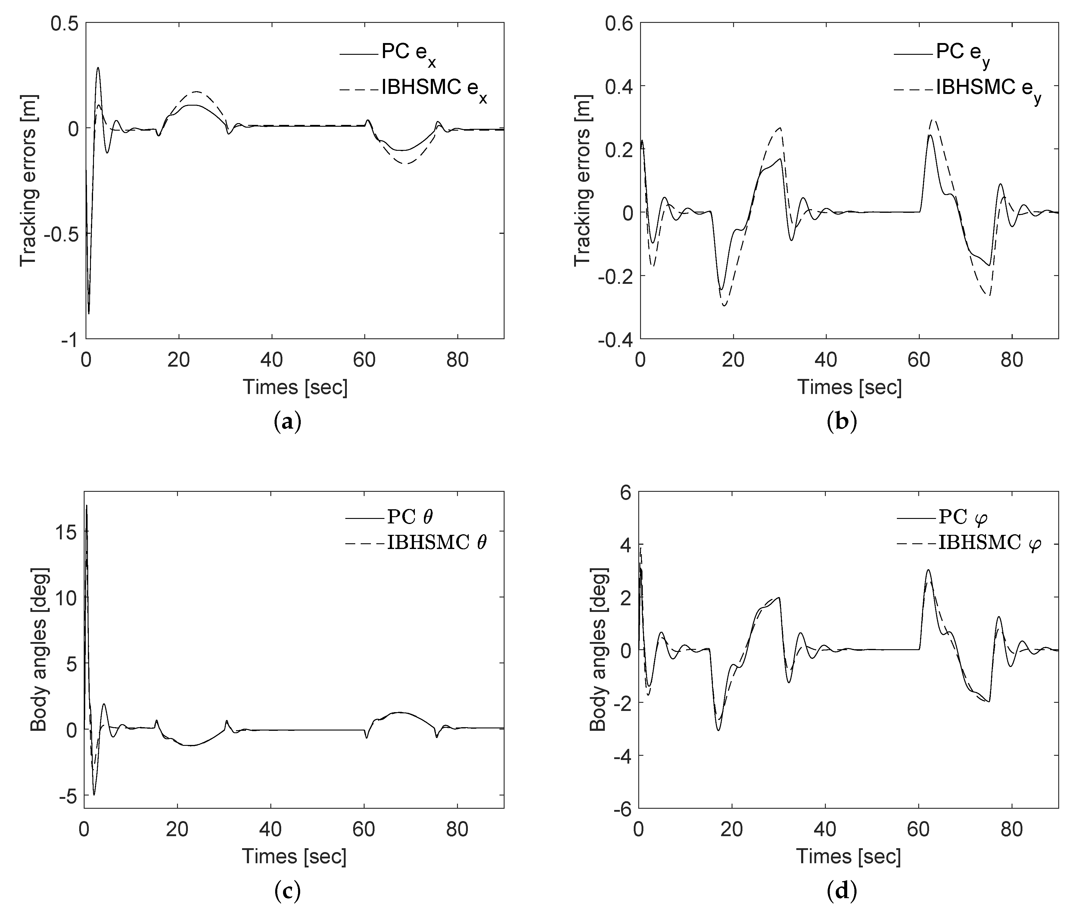
3.2. Simulation Results

This section presents the simulation results on the proposed method. The model parameters are given in

Table 1. Parameters of the ball-balancing robot [12].

Symbol	Parameter	Value
$m_b$	Body mass	$116\mathrm{kg}$
l	Body length	$0.23\mathrm{kg}$
$I_{bx}$	Moment of inertia of the body about the roll axis	$16.25\mathrm{kg}·{\mathrm{m}}^2$
$I_{by}$	Moment of inertia of the body about the pitch axis	$15.85\mathrm{kg}·{\mathrm{m}}^2$
$r_w$	Omnidirectional wheel radius	$0.1\mathrm{kg}$
$m_w$	Omnidirectional wheel mass	$0.56\mathrm{kg}$
$I_w$	Moment of inertia of the omnidirectional wheel	$0.26\mathrm{kg}$
$m_s$	Ball mass	$11.4\mathrm{kg}$
$r_s$	Ball radius	$0.19\mathrm{kg}$
$I_s$	Moment of inertia of the ball	$0.165\mathrm{kg}$
$\alpha$	Zenith angle	${56}^{\circ }$

. The design parameters were chosen as ${\mathit{K}}_1=\mathrm{diag}(10,10)$, ${\mathit{K}}_2=\mathrm{diag}(10,10)$, $\lambda =2$, ${\mathit{\lambda }}_{\theta }=\mathrm{diag}(-0.1,0.1)$, ${\sigma }_1={\sigma }_2=0.1$, and ${\tau }_1={\tau }_2=0.1$. The initial states of the robot were taken as $\mathit{q}={\left[\begin{array}{c}-0.2,0.2,0,0\end{array}\right]}^{\top }$. The friction parameters were chosen as ${\zeta }_x={\zeta }_y=2\mathrm{N}·\mathrm{s}/\mathrm{m}$ and ${\zeta }_{\theta }={\zeta }_{\phi }=1\mathrm{N}·\mathrm{s}/\mathrm{rad}$. To consider perturbed dynamics, we assumed that we knew the nominal parameters as follows: $m_b=116\mathrm{kg}$, $l=0.23\mathrm{m}$, $I_{bx}=16.25\mathrm{kg}·{\mathrm{m}}^2$, and $I_{by}=15.85\mathrm{kg}·{\mathrm{m}}^2$. To verify the performance of the proposed method, the reference trajectory was composed of straight lines and curves, and the proposed controller (PC) was compared with the integral backstepping hierarchical sliding mode control (IBHSMC) method [12].

The simulation results on the trajectory tracking are shown in Figure 2. It can be seen that both methods had precise tracking performance for straight paths and slight errors for curved paths. Figure 3 shows the detailed simulation results. The trajectory tracking errors of the ball-balancing robot are shown in Figure 3a,b, and the body angles of the robot are depicted in Figure 3c,d. It can be seen that neither method made a significant difference in balancing performance. On the other hand, in trajectory tracking, the proposed method showed a $19.2\%$ improved error rate compared to the IBHSMC method. Figure 4a,b shows the control inputs and estimates of the optimal weights for the RBFNs, respectively.

Table 2. RMS of tracking errors according to the control gain.

Gain	Nominal	Perturbed
$K_1=\mathrm{diag}(0.1,0.1)$	0.1299	0.2108
$K_1=\mathrm{diag}(1,1)$	0.1278	0.1355
$K_1=\mathrm{diag}(10,10)$	0.1271	0.1244

shows the root mean square (RMS) of the tracking errors for various control gains. This result sufficiently validated that the tracking and balancing errors can be made arbitrarily small by properly choosing the design parameters. From these results, we could demonstrate that the proposed method was effective in achieving simultaneous trajectory tracking and balancing of the ball-balancing robot.

4. Discussion

In this paper, a neural-network-based control method was proposed for trajectory tracking and balancing of a ball-balancing robot. We introduced a virtual angle to solve the underactuation problem and designed a single-loop controller using the DSC method for a simple control system. Moreover, we employed the RBFNs to compensate for the uncertainties and derived the update laws for the RBFNs in the Lyapunov sense. From the Lyapunov stability theorem, it was proven that all errors in the closed-loop control system were uniformly ultimately bounded and could be made arbitrarily small. The simulation results, including comparisons with the previous method, were provided to verify the performance of the proposed method. It was shown that the proposed method had a $19.2\%$ improved tracking error rate compared to the previous method. In addition, it was confirmed that all errors could be made arbitrarily small as the choice of the design parameters shown in Table 2. Therefore, unlike other previous studies, the proposed method had a simple control system structure and guaranteed stability in achieving simultaneous trajectory tracking and balancing.

In this paper, it was assumed that all states, such as the position, body angle, and velocity of the robot, were measurable and exact. However, this may not be practical because it requires many sensors and can be contaminated by noise. The output-feedback control method using the observer can be a solution to this problem. Therefore, as future research, we will provide a control method that minimizes the use of sensors, such as output-feedback control.

References

1. Paszkiel, S. Using the Raspberry PI2 Module and the Brain-Computer Technology for Controlling a Mobile Vehicle. In Automation 2019; Szewczyk, R., Zieli ’nski, C., Kaliczy ’nska, M., Eds.; Springer International Publishing: Cham, Switzerland, 2020; Volume 920, pp. 356–366. [Google Scholar]
2. Han, H.Y.; Han, T.Y.; Jo, H.S. Development of omnidirectional self-balancing robot. In Proceedings of the 2014 IEEE International Symposium on Robotics and Manufacturing Automation (ROMA), Kuala Lumpur, Malaysia, 15–16 December 2014; pp. 57–62. [Google Scholar]
3. Tsai, C.C.; Chan, C.K.; Kau, L.C. LQR Motion Control of a Ball Riding Robot. In Proceedings of the 2012 IEEE/ASME International Conference on Advanced Intelligent Mechatronics (AIM), Tokyo, Japan, 11–14 July 2012; pp. 861–866. [Google Scholar]
4. Lauwers, T.B.; Kantor, G.A.; Hollis, R.L. A dynamically stable single-wheeled mobile robot with inverse mouse-ball drive. In Proceedings of the 2006 IEEE International Conference on Robotics and Automation, Orlando, FL, USA, 15–19 May 2006; pp. 2884–2889. [Google Scholar]
5. Nagarajan, U.; Kantor, G.; Hollis, R. The ballbot: An omnidirectional balancing mobile robot. Int. J. Robot. Res. 2014, 33, 917–930. [Google Scholar] [CrossRef]
6. Pham, D.B.; Weon, I.S.; Lee, S.G. Partial feedback linearization double-loop control for a pseudo-2D ridable ballbot. Int. J. Control Autom. Syst. 2020, 18, 1310–1323. [Google Scholar] [CrossRef]
7. Pham, D.B.; Kim, H.; Kim, J.; Lee, S.G. Balancing and transferring control of a ball segway using a double-loop approach [applications of control]. IEEE Control Syst. Mag. 2018, 38, 15–37. [Google Scholar]
8. Wang, W.; Yi, J.; Zhao, D.; Liu, D. Design of a stable sliding-mode controller for a class of second-order underactuated systems. IEE Proc.-Control Theory Appl. 2004, 151, 683–690. [Google Scholar] [CrossRef] [Green Version]
9. Pham, D.B.; Lee, S.G. Hierarchical sliding mode control for a two-dimensional ball segway that is a class of a second-order underactuated system. J. Vib. Control 2019, 25, 72–83. [Google Scholar] [CrossRef]
10. Pham, D.B.; Lee, S.G. Aggregated hierarchical sliding mode control for a spatial ridable ballbot. Int. J. Precis. Eng. 2018, 19, 1291–1302. [Google Scholar] [CrossRef]
11. Do, V.T.; Lee, S.G.; Kim, J.H. Robust integral backstepping hierarchical sliding mode controller for a ballbot system. Mech. Syst. Signal Process. 2020, 144, 106866. [Google Scholar] [CrossRef]
12. Do, V.T.; Lee, S.G. Neural Integral Backstepping Hierarchical Sliding Mode Control for a Ridable Ballbot Under Uncertainties and Input Saturation. IEEE Trans. Syst. Man Cybern. Syst. 2021, 1–14. [Google Scholar] [CrossRef]
13. Park, K.B. Comments on ‘design of a stable sliding-mode controller for a class of second-order underactuated Systems’. IET Control Theory Appl. 2012, 6, 1153. [Google Scholar] [CrossRef]
14. Lee, S.M.; Park, B.S. Robust Control for Trajectory Tracking and Balancing of a Ballbot. IEEE Access 2020, 8, 159324–159330. [Google Scholar] [CrossRef]
15. Sands, T. Development of Deterministic Artificial Intelligence for Unmanned Underwater Vehicles (UUV). J. Mar. Sci. Eng. 2020, 8, 578. [Google Scholar] [CrossRef]
16. Fan, Y.; Huang, H.; Tan, Y. Robust adaptive path following control of an unmanned surface vessel subject to input saturation and uncertainties. Appl. Sci. 2019, 9, 1815. [Google Scholar] [CrossRef] [Green Version]
17. Sands, T. Deterministic Artificial Intelligence; IntechOpen: London, UK, 2020; ISBN 978-1-78984-111-4. [Google Scholar]
18. Tran, D.T.; Nguyen, M.N.; Ahn, K.K. RBF Neural Network Based Backstepping Control for an Electrohydraulic Elastic Manipulator. Appl. Sci. 2019, 9, 2237. [Google Scholar] [CrossRef] [Green Version]
19. Swaroop, D.; Hedrick, J.K.; Yip, P.P.; Gerdes, J.C. Dynamic surface control for a class of nonlinear systems. IEEE Trans. Autom. Control 2000, 45, 1893–1899. [Google Scholar] [CrossRef] [Green Version]
20. Ge, S.S.; Wang, C. Adaptive neural control of uncertain MIMO nonlinear systems. IEEE Trans. Neural Netw. 2004, 15, 674–692. [Google Scholar] [CrossRef] [PubMed]
Figure 1. Spatial model of the ball-balancing robot [10].
Applsci 11 04739 g001
Figure 2. Simulation results on the trajectory tracking performances of the ball-balancing robot.
Applsci 11 04739 g002
Figure 3. Simulation results (a) tracking error e x ; (b) tracking error e y ; (c) body angle θ ; (d) body angle φ .
Applsci 11 04739 g003
Figure 4. Simulation results (a) control inputs; (b) estimates of the optimal weights of the RBFNs (solid: ω ^ 1 , dotted: ω ^ 2 ).
Applsci 11 04739 g004