Article

Bearing Anomaly Recognition Using an Intelligent Digital Twin Integrated with Machine Learning

Department of Electrical, Electronics and Computer Engineering, University of Ulsan, Ulsan 44610, Korea
*
Author to whom correspondence should be addressed.
Appl. Sci. 2021, 11(10), 4602; https://doi.org/10.3390/app11104602
Submission received: 8 April 2021 / Revised: 12 May 2021 / Accepted: 14 May 2021 / Published: 18 May 2021
(This article belongs to the Collection The Development and Application of Fuzzy Logic)

Abstract

:

Featured Application

Bearing anomaly recognition using an intelligent digital twin integrated with machine learning.

Abstract

In this study, the application of an intelligent digital twin integrated with machine learning for bearing anomaly detection and crack size identification will be observed. The intelligent digital twin has two main sections: signal approximation and intelligent signal estimation. The mathematical vibration bearing signal approximation is integrated with machine learning-based signal approximation to approximate the bearing vibration signal in normal conditions. After that, the combination of the Kalman filter, high-order variable structure technique, and adaptive neural-fuzzy technique is integrated with the proposed signal approximation technique to design an intelligent digital twin. Next, the residual signals will be generated using the proposed intelligent digital twin and the original RAW signals. The machine learning approach will be integrated with the proposed intelligent digital twin for the classification of the bearing anomaly and crack sizes. The Case Western Reserve University bearing dataset is used to test the impact of the proposed scheme. Regarding the experimental results, the average accuracy for the bearing fault pattern recognition and crack size identification will be, respectively, 99.5% and 99.6%.

1. Introduction

The effort to reduce energy consumption has been one of the significant challenges in recent years. In this regard, heavy industries play a considerable role in energy consumption. Induction motors are the essential tools used in heavy industries and consume around 80% of the energy in these industries. To increase efficiency and reduce energy consumption in motors, various factors such as improving the quality of power consumption and condition monitoring for fault detection, identification, and tolerance play a constructive role. To examine faults in motors, it should be noted that in general, mechanical defects at about 79% and electrical faults at around 21% are the major fault groups in these systems. One of the remarkable types of mechanical faults is bearing failure, which accounts for about 69% of mechanical defects [1].
Nondestructive tests are extremely important for condition monitoring of bearings. The basic concept of nondestructive tests is analyzing the various types of signals extracted from bearings. Nondestructive test methods are evolving day by day, the most important of which are magnetic detection tests, sound and vibration tests, ultrasound, electromagnetic spectroscopy, signal processing, and multidimensional image processing. Each of these methods has special advantages that make them more suitable for use in various industries. Condition monitoring means fault diagnosis and maintenance from the operating bearing. In general, this method works based on data collection of dynamic properties of the bearing and comparing them with their healthy state. In classical condition monitoring, faults are usually detected by one of the following techniques: vibrations, acoustic emission, and motor current signature analysis [2]. In this work, the vibration sensor is used for data collection.
Different methods have been introduced for bearing-fault detection and identification (BFDI) and are categorized into the following four main groups: signal processing-based approaches, model-based schemes, machine/deep learning methods, and hybrid approaches [3,4]. Signal processing-based techniques have been used to diagnose defects in various studies, but robustness in noisy conditions is the principal challenge of these techniques [5,6]. On the other hand, model-based approaches are robust and stable, but modeling the physical systems in uncertain conditions is the main challenge of this method [7]. Most recently, machine/deep learning schemes have been applied in numerous applications, but reliability is the foremost challenge of these methods [4]. Hybrid algorithms are a combination of two or three of the above algorithms to make new reliable and effective techniques for BFDI [8]. In this research, a hybrid algorithm based on the incorporation of the model-based approach, data-driven technique, artificial intelligence method, and machine learning algorithm is prescribed.
Digital twins are important to confirm the style of a physical system. This basic concept is introduced to make a connection between the modeling and the real-time measurement from the systems. Moreover, the digital twin is used for state prediction [9]. To design a BFDI based on a digital twin (DT), the combination of the model-based approach, data-driven technique, artificial intelligence approach, and machine learning scheme is used. The central concept of a DT is designed based on physical system modeling. To model the real systems, diverse procedures have been used that are categorized into two principal groups: (i) mathematical-based system modeling such as the newton Euler technique, Lagrange method, and (ii) data-driven-based system modeling such as system identification techniques, artificial intelligence methods, machine learning approaches, and deep learning schemes [10]. Mathematical modeling for vibration signals in the bearings has been presented in [10,11]. The main affirmative point for vibration modeling in the bearing based on the mathematical-based approach (such as multi degrees of freedom vibration bearing modeling) is reliability. However, the complexity and difficulty of the modeling in the presence of uncertain conditions can be the most important challenge of this technique. To reduce the complexity of system modeling based on mathematical algorithms, data-driven approaches have been introduced [12,13]. The applications of the fuzzy technique in function approximation (system modeling) have been reported in [14]. Tuning the gain updating factors and membership functions are significant challenges of the classical fuzzy technique for function approximation. The next candidate for function approximation in nonlinear systems is a neural network. The applications of the neural network such as multilayer perceptron (MLP) and radial bases neural network for approximation of the system/signal have been proposed in [15]. In recent years, the application of machine and deep learning for function approximation has increased sharply. The application of a machine learning-based approach such as support vector regression for signal approximation has been introduced in [16]. Recently, deep learning methods such as convolutional neural networks [17], recurrent neural networks [18], generative adversarial networks [19], self-organizing maps [20], Boltzmann machines [21], deep reinforcement learning [22], and autoencoders [23] have been highly recommended for function approximation. The next algorithms for function approximation are identification techniques. These techniques work based on the combination of modern control algorithms and regression techniques. The identification algorithms are categorized into two groups: a linear approach and a nonlinear approach [24]. In the linear based identification technique, the linear function based on the regression technique is used to approximate the function of systems. In the nonlinear-based identification technique, the nonlinear functions based on a combination of the identification algorithm, artificial intelligence, and modern control algorithm are used to approximate the function of systems [17]. In this research, a combination of mathematical-based modeling and a nonlinear-based identification algorithm for modeling the DT of the bearing is recommended.
To increase the accuracy of modeling in DT, various techniques can be used such as observation techniques and the Kalman filter method [25]. The observation techniques are categorized into two general groups: (i) linear observers such as proportional-integral (PI) observer [26] and proportional multi-integral (PMI) observer [27]; (ii) nonlinear observers such as sliding mode observer (SMO) [10,28], feedback linearization observer (FLO) [29], backstepping observer (BSO) [30], fuzzy observer (FO) [31], neural network observer (NNO) [32], and Lyapunov observer (LO) [33]. However, the main advantage of the linear observer is simplicity, while accuracy is the main challenge of this algorithm. The FLO and the BSO have solved the challenge of estimation accuracy, but robustness was the challenge in these techniques. To reduce the challenge of robustness, SMO and LO have been used in different applications. The challenge of classical SMO is the chattering phenomenon. The LO also has the challenge of complexity. The FO and the NNO have the challenge of reliability for signal estimation. The second way to estimate the signal is the Kalman filter (KF) technique. The KF assumes that the noise is distributed Gaussian, and the signal observation models are linear [34]. Nevertheless, the filter gives the succeeding conditional probability estimate in the particular case where the errors follow a Gaussian distribution. The main drawback of the KF for signal estimation is the performance of this algorithm against nonlinear signals. Over the years, generalizations and extensions to this method have been established, such as the unscented Kalman filter (UKF) and the extended Kalman filter (EKF) in which both techniques are worked based on a linearization algorithm [35]. The extended Kalman filter is the most widely used estimation algorithm for nonlinear systems based on a linearization algorithm [33]. In the linearization technique, the accuracy of signal estimation is not accurate enough for signal estimation for fault pattern recognition and crack size identification (FPRCI). To develop the performance of signal estimation including reducing the estimation error in normal conditions and increasing the level of separability for FPRCI, the hybrid-based Kalman filter (HBKF), which is a combination of the Kalman filter, a high-order variable structure uncertainties estimator, hybrid-based signal modeling, and adaptive neural-fuzzy technique, will be introduced here.
After estimating the vibration signals, the classification algorithms can be selected for FPRCI. To classify the signal’s state different techniques have been used that are divided into three main groups: (a) classical classifiers such as the sliding mode technique [10]; (b)machine learning-based classifiers including support vector machine (SVM) [36] and decision trees [37]; (c) deep learning-based classifiers including convolution neural networks [38] and autoencoders [39]. In this work, the SVM is recommended for classification of the faults and identification of the crack sizes.
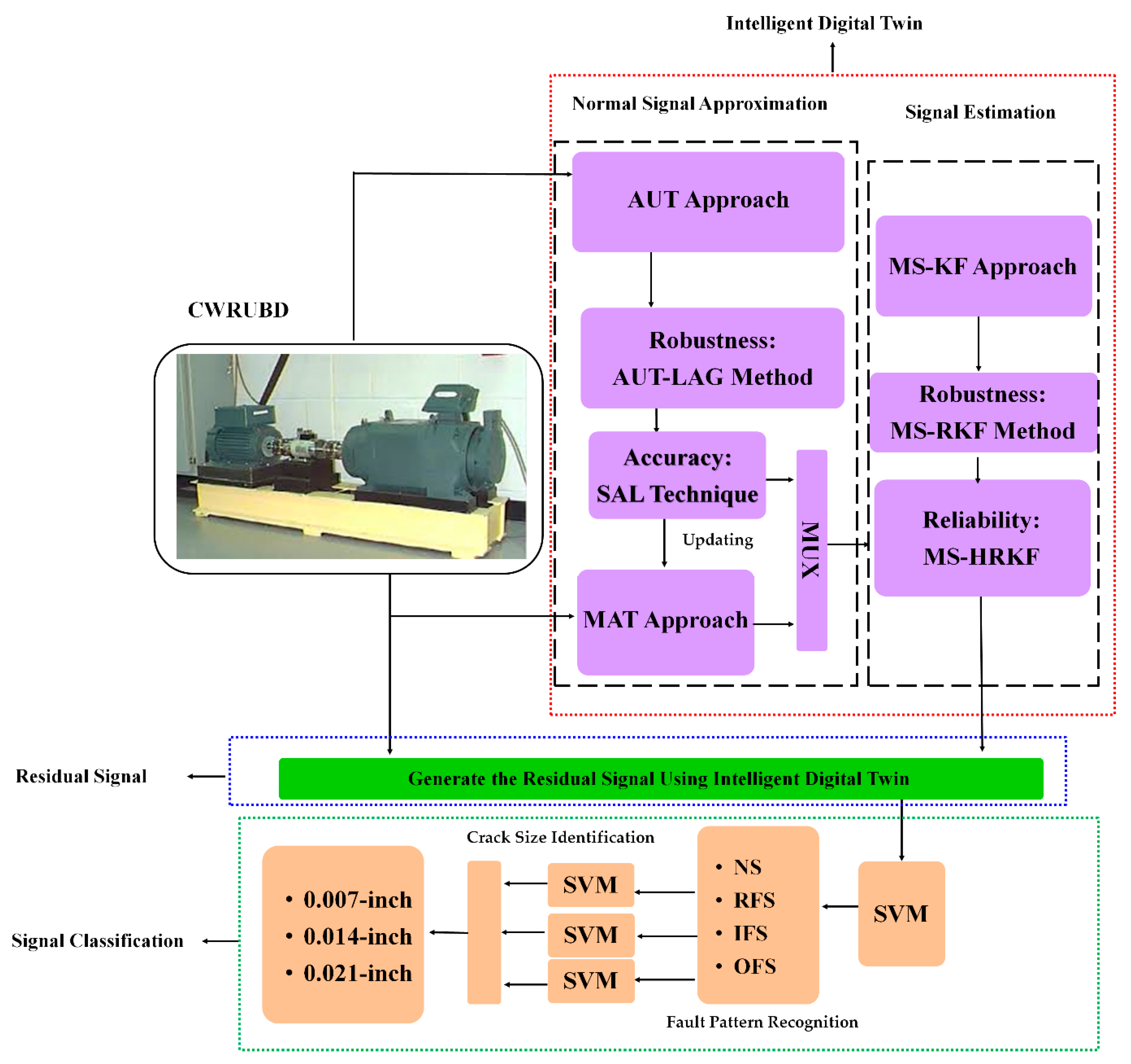
In this research, the combination of the hybrid-based signal modeling, an adaptive neural-fuzzy-based variable structure Kalman filter, and SVM is suggested for FPRCI. Thus, this technique has three stages: signal approximation and estimation using the intelligent DT technique, residual signal generation, and classification. The first stage (intelligent digital twin) has two parts: (a) signal approximation and (b) signal estimation. Therefore, first, the normal signal is approximated using a combination of the mathematical-based approach and machine learning-based regression. Next, the combination of a Kalman filter (KF), the high-order variable structure technique (HVS), and the adaptive neural-fuzzy method (ANF) are recommended in this research, which from now on is called the hybrid robust Kalman filter (HRKF) for signal estimation. In the next stage, the residual signal is generated using the difference between the original and the estimated vibration signals. In addition, in the third stage, an SVM is suggested for FPRCI. This work has the following contributions:
  • The vibration signal approximation using a combination of the mathematical-based approach and machine learning-based regression is the first contribution of this work.
  • The vibration bearing signal estimation using intelligent DT based on the combination of a Kalman filter, the high-order variable structure technique, and the adaptive neural-fuzzy method (ANF) that is approximated using the proposed approach.
  • The anomaly classification and crack size identification using intelligent DT integrated with machine learning approach is the third contribution.
This research work has the following parts. The proposed digital twin integrated with the machine learning approach is proposed in Section 2. Section 3 provides experimental results for the proposed digital twin integrated with the machine learning approach as compared with the other approaches. The conclusion is explained in Section 4.

2. Proposed Methodology

Figure 1 illustrates the intelligent DT integrated with SVM for FPRCI. Based on this figure, the combination of the proposed signal approximation algorithm, adaptive neural-fuzzy integrated with variable structure Kalman filter, and SVM is recommended for FPRCI. Thus, the intelligent DT (signal approximation and estimation), residual signal generation, and classification are the three main stages in the proposed algorithm.
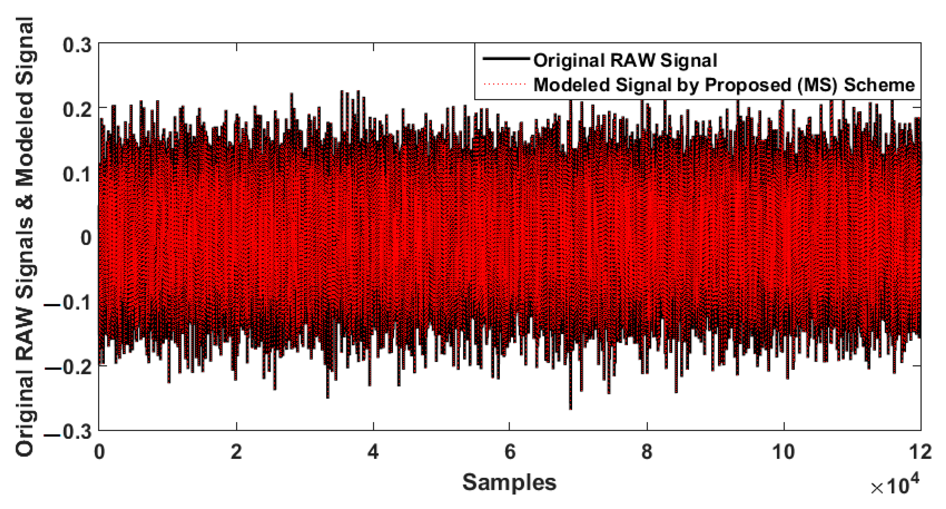
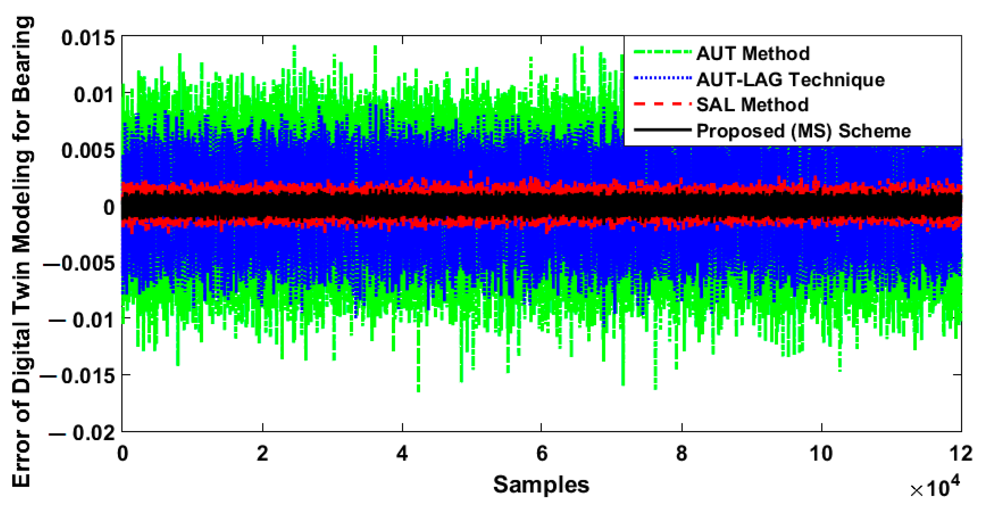
In the first stage, the proposed intelligent DT is designed. This part has two sub-blocks, the signal approximation unit and the signal estimation unit. For normal signal approximation, the mathematical vibration signal modeling is integrated with the data-driven algorithm. The data-driven-based regression is designed based on the combination of the autoregression technique, the Laguerre method, and the machine learning-based (support vector regression (SVR)) approach (henceforth called SAL). Therefore, from now on the combination of the mathematical-based modeling (MAT) and SAL algorithm is called MS. For vibration signal estimation, the hybrid robust Kalman filter (HRKF) is proposed. The HRKF is the combination of the Kalman Filter (KF), the high-order variable structure technique (HVS), and the adaptive neural-fuzzy method (ANF). Thus, first, the KF is developed based on the normal signal state-space signal modeling. Next, The HVS technique is suggested to reduce the error of signal modeling in uncertain conditions. After that, the combination of the KF and the HVS with the ANF method is used to increase the reliability and flexibility of the normal signal estimation.
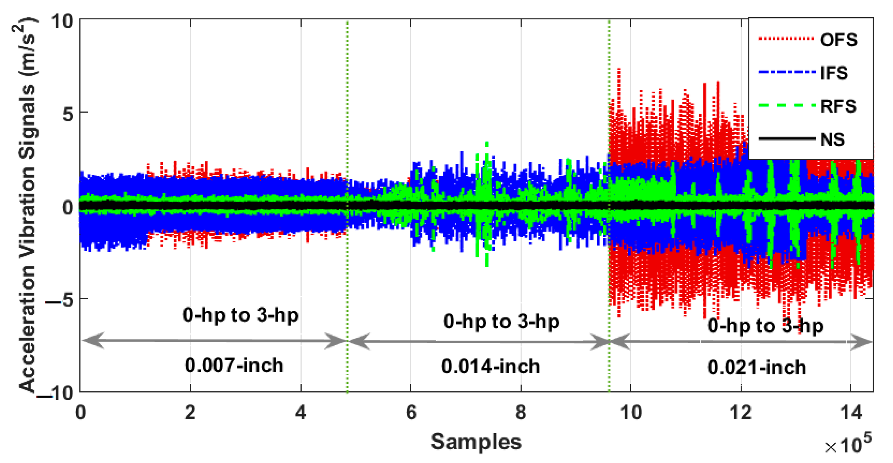
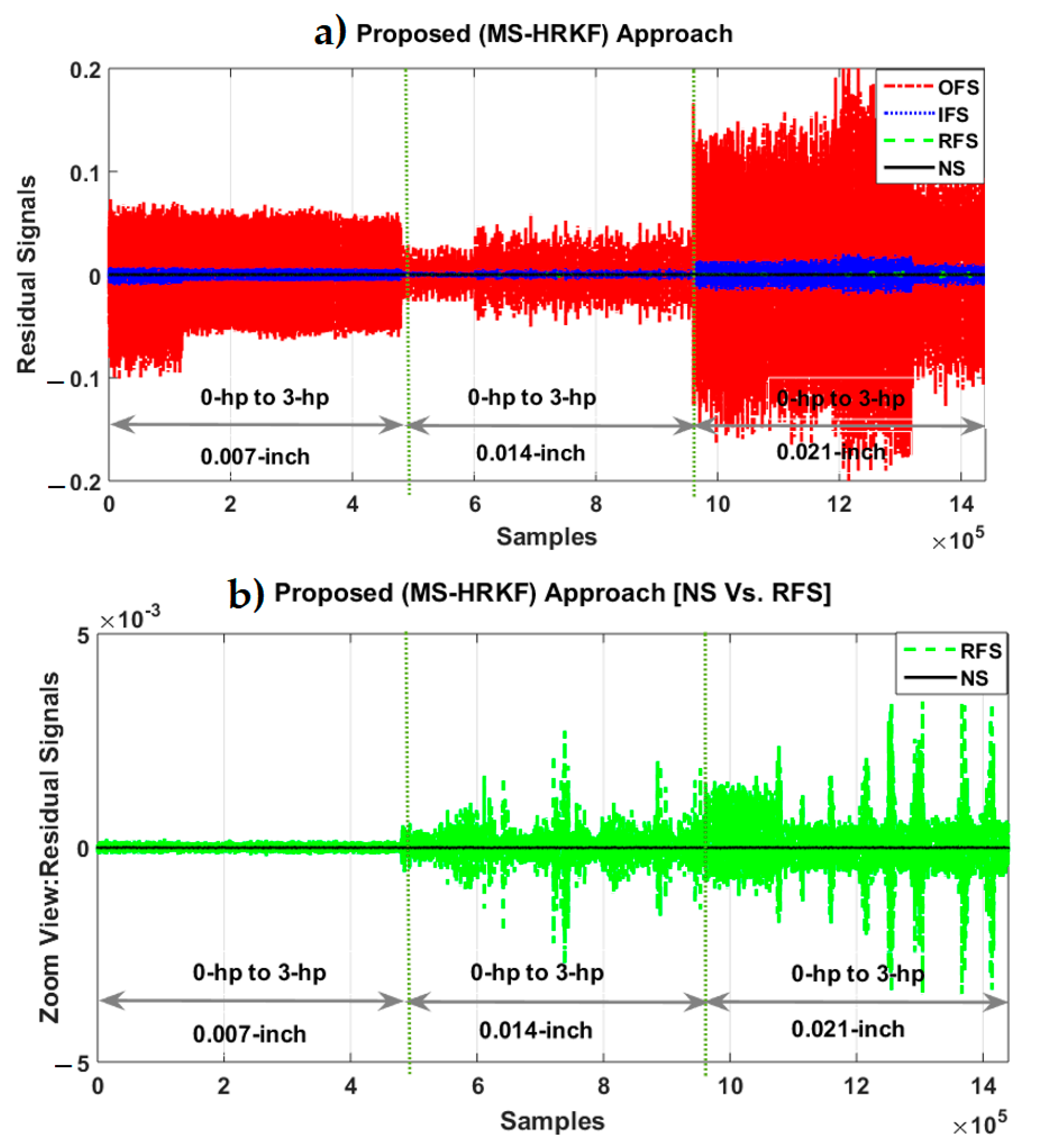
Thus, the proposed intelligent DT is developed by MS integrated with the HRKF. The second stage is the residual signal generation based on the difference between the original RAW signals and the estimated ones. The level of residual signals in different patterns is completely different. In addition, the different crack sizes have different signal levels. Thus, the level of residual signals for normal (NS), roller fault state (RFS), inner fault state (IFS), and outer fault state (OFS) are different, which from now on is called fault pattern recognition. Moreover, the level of these signals in the various crack sizes (0.007, 0.014, and 0.021 inch) are different, which from now on is called crack size identification.
The third stage is used for the classification of residual signals based on the machine learning approach. Thus, the SVM is used for FPRCI.

2.1. Dataset

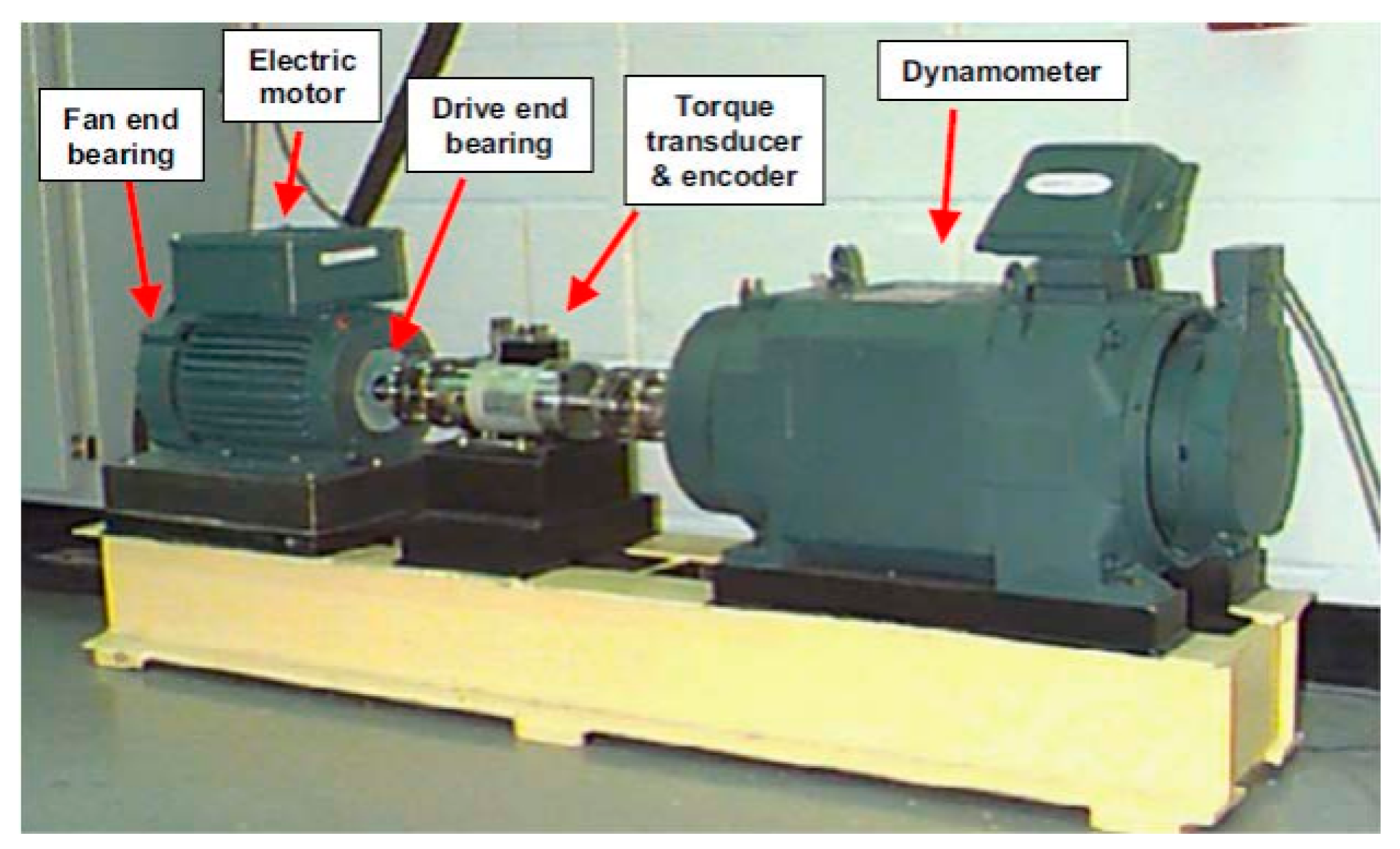
The Case Western Reserve University bearing dataset (CWRUBD) is recommended to test the proposed intelligent digital twin technique for FPRCI in the bearing. In the CWRUBD, a 2 horsepower (hp) reliance electric motor drives a shaft on which a torque transducer and encoder are mounted. Torque is applied to the shaft via a dynamometer and electronic control system. A motor is utilized to rotate the bearing at four different rotation per minute (RPM) speeds—including 1797, 1772, 1750, and 1730 RPM [38]. Vibration data was collected using accelerometers, which were attached to the housing with magnetic bases. Accelerometers were placed at the 12 o’clock position at both the drive end and fan end of the motor housing. During some experiments, an accelerometer (PCB 353B33 accelerometers-PCB Piezotronics) was attached to the motor supporting base plate as well. Vibration signals were collected using a 16-channel data acquisition module NI DAQ 6062E recorder and were post processed in a MATLAB environment. The vibration signals were collected via installed on bearing housing. A vibration sensor is used to collect the data in four different conditions including NS, RFS, IFS, and OFS, with three different crack sizes including 0.007, 0.014, and 0.021 inch. Moreover, the sampling rate of data collection is 48 kHz. The bearing type used in the CWRUBD is the 6205-2RS JEM SKF roller bearing. Figure 2 shows the testbed for data collection which is designed by CWRUBD. Moreover, Table 1 summarizes the information of the CWRUBD according to the signal conditions, motor torque loads, and the bearing crack sizes [40].

2.2. Digital Twin

Designing an intelligent digital twin has two parts: (a) signal approximation using a combination of mathematical-based vibration signal of bearing modeling with machine learning-based regression, and (b) signal estimation to improve the performance of signal modeling using the combination of a Kalman filter, the high-order variable structure technique, and the adaptive neural-fuzzy method (ANF).

2.2.1. Signal Modeling: The First Step to Design the Digital Twin

The first part of this stage is the vibration signal modeling in the normal state for the bearing. Therefore, first, the vibration signal in the normal state using the five degrees of freedom (DOF) mathematical Lagrangian technique is modeled. The mathematical vibration signal modeling for the bearing in the normal state is expressed by the following function [10,41].
f M ( q ) = M M ( q ) [ q ¨ ] + B M ( q , q ˙ ) + Δ M
Here, f M ( q ) , M M ( q ) , q ¨ , B M ( q , q ˙ ) , and Δ M are the force applied to the bearing, the matrices of mass for the bearing, the vibration signal acceleration for the bearing, the nonlinear term of the vibration signal that is one of the important challenges for mathematical modeling, and unknown conditions including faults and uncertainties, respectively. The nonlinear term of the vibration signal should be calculated using the following definition.
B M ( q , q ˙ ) = V M [ q ˙ ] + D M [ q ]
Here, V M , q ˙ , and D M are the stiffness of the bearing which is a nonlinear-based parameter, the velocity of the vibration signal of the bearing, and the damping of the bearing, respectively. Regarding (1), estimation of the parameter of the unknown condition is one of the main challenges of mathematical modeling of nonlinear systems such as the bearing. Therefore, based on [10,41], the unknown conditions that are a combination of uncertainties and faults can be modeled using 5-DOF vibration signal modeling, and is defined by the following equation.
Δ M = α r + α i + α o
where α r , α i , and α o are the predicted effect of RFS, IFS, and OFS, respectively. The predicted RFS effect, IFS effect, and OFS effect are represented as the following definitions, respectively.
α r = M a x ( α i o C o s ( α j ) + α i o S i n ( α j ) ϵ ω α f , 0 )
α i = M a x ( α i o C o s ( α j ) α i o S i n ( α j ) ( 2 × ( ϵ ω α f ) ) , 0 )
α o = M a x ( α i o C o s ( α j ) + 1.5 × α i o S i n ( α j ) ϵ ω + α f , 0 )
where the difference between the center of mass in IFS and OFS, ( α i o ) , is represented as follows:
α i o = α x i α x o
Here, α x i and α x o are the IFS center of mass and the OFS center of mass, respectively. The angular position in the RFS, IFS, and OFS, ( α j ) , is computed as the following equation.
α j = 2 π ( j 1 ) k r + ϵ ω + α o
where k r   and   ϵ ω are the RFS numbers and the rotor velocity, respectively. Moreover, the deformation, ( α f ) , is determined as follows:
α f = ϵ ω a + ϵ ω b
Here, ( ϵ ω a and ϵ ω b ) are the angular width at two positions, position a and b, respectively. Thus, regarding (1), the state-space function for modeling the bearing in the healthy state based on the mathematical technique using 5-DOF vibration signal modeling is represented by the following definition.
{ W M A T ( k + 1 ) = γ M A T ( W M A T ( k ) , U i n ( k ) ) + Δ ( W M A T ( k ) , U i n ( k ) ) Z M A T ( k ) = ( β M A T ) T W M A T ( k )
Here,   W M A T ( k ) , U i n ( k ) , γ M A T ( W M A T ( k ) , U i n ( k ) ) , Z M A T ( k ) , β M A T , and Δ ( W M A T ( k ) , U i n ( k ) ) are the state of the bearing signal, the input signal that should be measured, the nonlinearity term for the bearing modeling using the 5-DOF vibration signal, the output of the signal’s model using 5-DOF vibration signal modeling, the coefficient to optimize the state-space output, and finally the unknown conditions, respectively. Table 2 illustrates the bearing parameter information to the mathematical modeling of the bearing that was collected by CWRUBD. This procedure is reliable, but the complexity and uncertain condition modeling are the two main problems of the mathematical system modeling to design the digital twin.
In the next step, the data-driven system identification technique is suggested to modify the accuracy of system modeling for the bearing digital twin. Thus, regarding Figure 1, first, the autoregressive technique is recommended to approximate the state-space function of the vibration signal of the bearing in the normal state. The autoregressive (AUT) technique is a linear-based signal approximation for modeling the signal in different domains such as state-space. Thus, the state-space bearing signal modeling in a healthy condition is represented as follows [42].
{ W A U T ( k + 1 ) = [ γ A U T W A U T ( k ) + Δ A U T ( k ) ] + e A U T ( k ) Z A U T ( k ) = ( β A U T ) T W A U T ( k )
Here, W A U T ( k ) , e A U T ( k ) , Δ A U T ( k ) ,   Z A U T ( k ) , and ( γ A U T , β A U T ) are the state of the signal modeling based on the AUT technique for the bearing’s digital twin, the error of the bearing’s digital twin modeling using the AUT technique, the unknown condition of the bearing’s digital twin modeling that is computed using the AUT technique, the bearing’s digital twin output modeling using the AUT technique, and the coefficients for the state-space bearing’s digital twin tuning using the AUT method, respectively. Moreover, the unknown condition and the error of the bearing’s digital twin modeling that are computed using the AUT technique are represented as follows.
{ Δ A U T ( k ) = Z ( k ) Z A U T ( k ) e A U T ( k ) = Z A U T ( k + 1 ) Z A U T ( k )
Here, Z ( k ) is the bearing RAW signal in the healthy state. The AUT technique is linear. To increase the robustness and reduce the effect of uncertain conditions, which was a challenge in mathematical modeling, and the AUT method of the digital twin, the robust autoregressive-Laguerre (AUT-LAG) technique is suggested. The state-space definition of the AUT-LAG method for the bearing’s digital twin modeling is represented as the following equation.
{ W A U T L A G ( k + 1 ) = [ γ A U T L A G 1 W A U T L A G ( k ) + γ A U T L A G 2 Z A U T L A G ( k ) + Δ A U T L A G ( k ) ] + e A U T L A G ( k ) Z A U T L A G ( k ) = ( β A U T L A G ) T W A U T L A G ( k )
Here, W A U T L A G ( k ) , e A U T L A G ( k ) , Δ A U T L A G ( k ) ,   Z A U T L A G ( k ) , and ( γ A U T L A G 1 , γ A U T L A G 2 , β A U T L A G ) are the state of the signal modeling based on the AUT-LAG technique for the bearing’s digital twin, the error of the bearing’s digital twin modeling using the AUT-LAG technique, the unknown condition of the bearing’s digital twin modeling that is computed using the AUT-LAG technique, the bearing’s digital twin output modeling using the AUT-LAG technique, and the coefficients for the state-space bearing’s digital twin tuning using the AUT-LAG method, respectively. Furthermore, the unknown condition and the error of the bearing’s digital twin modeling that are computed using the AUT-LAG technique are represented as the following calculation.
{ Δ A U T L A G ( k ) = Z ( k ) Z A U T L A G ( k ) e A U T L A G ( k ) = Z A U T L A G ( k + 1 ) Z A U T L A G ( k )
The AUT-LAG technique is more robust and stable than the AUT method, but this technique suffers from the nonlinear behavior of the signal. The machine-learning algorithm based on the support vector regression (SVR) is recommended to improve the effectiveness of the bearing’s digital twin modeling. Hence, the combination of AUT-LAG and SVR (henceforth called SAL) to identify the signal of the bearing is represented as the following function.
{ W S A L ( k + 1 ) = [ γ S A L 1 W S A L ( k ) + γ S A L 2 { Z A U T L A G ( k ) + Z S V R ( k ) } + Δ S A L ( k ) ] + e S A L ( k ) Z S A L ( k ) = ( β S A L ) T W S A L ( k )
Here, W S A L ( k ) , e S A L ( k ) , Δ S A L ( k ) ,   Z S A L ( k ) , Z S V R ( k ) , and ( γ S A L 1 , γ S A L 2 , β S A L ) are the state of the signal modeling based on the SAL technique for the bearing, the error of the bearing modeling using the SAL technique, the unknown condition of the bearing modeling that is computed using the SAL technique, the bearing output modeling using the SAL technique, the nonlinearity compensator of the bearing’s output compensation using the SVR technique, and the coefficients for the state-space bearing’s performance tuning using the SAL method, respectively. Additionally, the unknown condition and the error of the bearing’s modeling that are computed using the SAL procedure are represented as the following function.
{ Δ S A L ( k ) = Z ( k ) Z S A L ( k ) e S A L ( k ) = Z S A L ( k + 1 ) Z S A L ( k ) .
The nonlinearity compensator of the bearing’s output compensation using the SVR technique, ( Z S V R ( k ) ) , is introduced using the following definition.
Z S V R ( k ) = i ( δ i + δ i ) K ( θ i , θ ) + .
Here, ( δ i + , δ i ) , K ( θ i , θ ) , and are the Lagrange constants, the nonlinear kernel functions that are selected in this work to improve the power of compensation, and the function’s bias, respectively. The Gaussian kernel function is suggested in this work and this function is introduced based on variance, ( σ ) , using the following equation.
K ( θ i , θ ) = e ( 1 2 σ 2 θ i θ 2 ) .
In addition, the function’s bias ( ) is made known to the following preparation.
= 1 | S | s S [ Z S i S ( δ i + δ i ) × K ( θ i , θ S ) ( × s i g n ( δ i + δ i ) ) ] .
Here, S ,   Z S , and are the support vector of approximation, the signal which is defined in the range of the support vector, and the accepted boundary of the support vector to allow for better signal compensation, respectively. Furthermore, if ω is defined as a constant, the support vector of approximation, ( S ) , is defined using the following definition.
S = { i | 0 < δ i + δ i < ω } .
Thus, the proposed technique of the digital twin to model the bearing using the combination of the MAT technique, Equation (10) and the SAL algorithm, and Equation (15), (henceforth called MS) is represented as the following definition.
{ W M S ( k + 1 ) = [ γ M S 1 W M S ( k ) + γ M S 2 Z M S ( k ) + Δ M S ( k ) ] + e M S ( k ) Z M S ( k ) = ( β M S ) T W M S ( k ) .
Furthermore, the unknown condition and the error of the bearing modeling using the digital twin algorithm that was computed using the MS procedure are represented as the following function.
{ Δ M S ( k ) = Z ( k ) Z M S ( k ) e M S ( k ) = Z M S ( k + 1 ) Z M S ( k )
Here, W M S ( k ) , e M S ( k ) , Δ M S ( k ) ,   Z M S ( k ) , and ( γ M S 1 , γ M S 2 , β M S ) are the state of the bearing signal modeling based on the MS technique for the bearing’s digital twin, the error of the bearing’s digital twin modeling using the MS technique, the unknown condition of the bearing’s digital twin modeling that was computed using the MS technique, the bearing’s digital twin output modeling using the MS technique, and the coefficients for the state-space bearing’s digital twin performance tuning using the MS method, respectively.

2.2.2. Signal Estimation: Second Step to Design the Digital Twin

After the first step of the digital twin’s modeling for the bearing, in the next step, the signal estimation technique is suggested to improve the accuracy and robustness of the bearing’s digital twin. In this study, the hybrid robust Kalman filter, which is a combination of the Kalman filter (KF), the high-order variable structure technique (HVS), and the adaptive neural-fuzzy method (ANF) is recommended for signal estimation. Thus, first, we implement a Kalman filter for vibration signal estimation based on the MS signal modeling. The state-space KF formulation using the MS function approximation is represented as the following equation.
{ W M S K F ( k + 1 ) = [ γ M S 1 K F W M S K F ( k ) + γ M S 2 K F Z M S K F ( k ) + Δ M S K F ( k ) ] + e M S K F ( k ) + [ Z ( k ) Z M S K F ( k ) ] Z M S K F ( k ) = ( β M S K F ) T W M S K F ( k )
Here, W M S K F ( k ) , e M S K F ( k ) , Δ M S K F ( k ) ,   Z M S K F ( k ) , , and ( γ M S 1 K F , γ M S 2 K F , β M S K F ) are the state of the signal estimation based on the KF technique for the bearing’s digital twin which was modeled by the MS technique, the error of the bearing’s digital twin estimation using the KF technique which was modeled by the MS technique, the unknown condition of the bearing’s digital twin estimation that was computed using the KF technique which was modeled by the MS technique, the bearing’s digital twin output estimation using the KF technique which was modeled by the MS technique, the Kalman filter gain matrices, and the coefficients for the state-space bearing’s digital twin tuning using the KF method which was modeled by the MS technique, respectively. Moreover, the Kalman filter gain matrices ( ) are represented as the following function.
( k ) = γ M S 1 K F × Δ M S K F ( k ) × ( β M S K F ) T [ β M S K F × Δ M S K F ( k ) × ( β M S K F ) T + N ]
Furthermore, to modify the performance of the KF estimator, the unknown condition of the bearing’s digital twin estimation that was computed using the KF technique which was modeled by the MS technique is represented using the following definition.
Δ M S K F ( k + 1 ) = γ M S 1 K F × Δ M S K F ( k ) × ( γ M S 1 K F ) T + Q ( k ) × [ β M S K F × Δ M S K F ( k ) × ( β M S K F ) T + N ] × T ( k )
Here, N and Q are the sensor noise and the process noise covariance matrices. To increase the accuracy and robustness of the KF, the combination of the KF and the HVS (henceforth called RKF) is recommended in this study. The robustness of the RKF to parameters of unknown conditions is guaranteed. Thus, the state-space RKF formulation using the MS function approximation is represented as the following calculation.
{ W M S R K F ( k + 1 ) = [ γ M S 1 R K F W M S R K F ( k ) + γ M S 2 R K F Z M S R K F ( k ) + Δ M S R K F ( k ) ] + e M S R K F ( k ) + [ Z ( k ) Z M S R K F ( k ) ] + γ M S 3 R K F × s g n ( S * R K F ) Z M S R K F ( k ) = ( β M S R K F ) T W M S R K F ( k )
where the sign function, ( s g n ( S * ) ) , is introduced as
{ s g n ( S * ) = 1                                               i f   S * 0 s g n ( S * ) = 1                                       i f   S * < 0 .
Besides, the unknown condition of the bearing’s digital twin estimation that was computed using the RKF technique and was modeled by the MS technique is represented using the following definition.
Δ M S R K F ( k + 1 ) = γ M S 1 R K F × Δ M S R K F ( k ) × ( γ M S 1 R K F ) T + Q ( k ) × [ β M S R K F × Δ M S R K F ( k ) × ( β M S R K F ) T + N ] × T ( k ) + γ M S 4 R K F × s g n ( S * R K F ) 0.5 φ R K F
and
φ ˙ R K F = γ M S 5 R K F × s g n ( S * )
Moreover, the surface of the variable structure method in the RKF, ( S * R K F ) , is represented as the following explanation.
S * R K F = Z Z M S R K F ( k )
Here, W M S R K F ( k ) , e M S R K F ( k ) , Δ M S R K F ( k ) ,   Z M S R K F ( k ) , S * R K F , and ( γ M S i R K F , β M S R K F ) are the state of the signal estimation based on the RKF technique for the bearing’s digital twin which was modeled by the MS technique, the error of the bearing’s digital twin estimation using the RKF technique which was modeled by the MS technique, the unknown condition of the bearing’s digital twin estimation that was computed using the RKF technique which was modeled by the MS technique, the bearing’s digital twin output estimation using the RKF technique which was modeled by the MS technique, the surface of the variable structure method in the RKF, and the coefficients for the state-space bearing’s digital twin tuning using the RKF method which was modeled by the MS technique, respectively. However, the RKF improves the robustness of the KF to increase the flexibility and accuracy of the bearing’s digital twin. The combination of the RKF and the ANF technique (henceforth called HRKF) modeled by the MS approach is recommended. The ANF approach is an artificial intelligence-based technique that is a combination of two approaches, a fuzzy logic algorithm and a neural network. Hence, the state-space HRKF formulation using the MS function approximation is represented as the following definition.
{ W M S H R K F ( k + 1 ) = [ γ M S 1 H R K F W M S H R K F ( k ) + γ M S 2 H R K F Z M S H R K F ( k ) + Δ M S H R K F ( k ) ] + e M S H R K F ( k ) + [ Z ( k ) Z M S H R K F ( k ) ] + γ M S 3 H R K F × s g n ( S * H R K F ) Z M S H R K F ( k ) = ( β M S H R K F ) T W M S H R K F ( k )
Above and beyond, the unknown condition of the bearing’s digital twin estimation that was computed using the HRKF technique and was modeled by the MS technique is represented using the following definition.
Δ M S H R K F ( k + 1 ) = γ M S 1 H R K F × Δ M S H R K F ( k ) × ( γ M S 1 H R K F ) T + Q ( k ) × [ β M S H R K F × Δ M S H R K F ( k ) × ( β M S H R K F ) T + N ] × T ( k ) + γ M S 4 H R K F × s g n ( S * H R K F ) 0.5 φ H R K F + γ M S 6 H R K F × Z A N F ( k )
and
φ ˙ H R K F = γ M S 5 R K F × s g n ( S * H R K F )
Moreover, the surface of the variable structure method in the HRKF, ( S * H R K F ) , is represented as the following explanation.
S * H R K F = Z Z M S H R K F ( k )
Here, W M S H R K F ( k ) , e M S H R K F ( k ) , Δ M S H R K F ( k ) ,   Z M S H R K F ( k ) , S * H R K F , Z A N F ( k ) , and ( γ M S i H R K F , β M S H R K F ) are the state of the signal estimation based on the HRKF technique for the bearing’s digital twin which was modeled by the MS technique, the error of the bearing’s digital twin estimation using the HRKF technique which was modeled by the MS technique, the unknown condition of the bearing’s digital twin estimation that was computed using the HRKF technique which was modeled by the MS technique, the bearing’s digital twin output estimation using the HRKF technique which was modeled by the MS technique, the surface of the variable structure method in the HRKF, the estimation compensator using the ANF method, and the coefficients for the state-space bearing’s digital twin tuning using the HRKF method which was modeled by the MS technique, respectively. The artificial intelligence-based technique, (ANF), to compensate the performance of the bearing’s digital twin output, ( Z A N F ( k ) ) , is introduced using the following definition.
{ Z A N F ( k ) = r Z r × ϑ r r ϑ r ϑ r = r e ( 0.5 i ( X ( k ) μ r σ ) 2 )
Here, Z r ( k ) , μ r , and σ are the reference point of uncertainty estimation using the ANF technique, the membership function of the fuzzy set to design the proposed ANF, and variance, respectively. To improve the performance of Z A N F ( k ) , the adaptive membership function and the adaptive variance of the fuzzy set to design the proposed ANF, ( μ r * )   and   ( σ * ) are defined as the following equations, respectively.
μ r , t + 1 * = μ r , t Θ r , t × ϑ r μ r , t
σ t + 1 * = σ t Θ r , t × ϑ r σ t
Here, Θ r , t is a tuning coefficient. Therefore, to design the digital twin for the bearing, we have two steps: signal modeling and signal estimation. For the first step of the bearing’s digital twin, signal modeling, the combination of autoregression (AR), Laguerre filter (LA), and support vector regression (SVR) (henceforth called SAL), was recommended. Next, in the second step of the bearing’s digital twin (signal estimation), the combination of a Kalman filter (KF), the high-order variable structure technique for robustness (R), and the adaptive neuro-fuzzy technique (ANF) (henceforth called HRKF), which was modeled by the SAL technique, was recommended. Consequently, after modeling and estimation the bearing signal using the proposed digital twin (MS-HRKF), the residual signal is computed in the next section.

2.3. Residual Signal Generation

Regarding Figure 1, the digital twin was used to model and estimate the signals. First, the normal condition signal was modeled using the proposed MS technique. Next, the estimator was designed and tuned for the normal state signal using the HRKF method. After that, the normal and abnormal state (unknown) signals were estimated using the proposed digital twin (MS-HRKF) scheme. The accuracy, robustness, and reliability of the digital twin are quite significant for signal classification. Before the signal classification using the machine learning algorithm, the residual signal, which is defined by the difference between the original RAW signal of the bearing and the estimated signal using the digital twin, is computed using the following formulation.
R M S H R K F ( k ) = Z ( k ) Z M S H R K F ( k )
where R M S H R K F ( k ) is the residual signal of unknown signals using the proposed digital twin (MS-HRKF) technique. In the next part, the machine learning technique is used for FPRCI of the bearing.

2.4. Fault Pattern Recognition and Crack Size Identification Using SVM

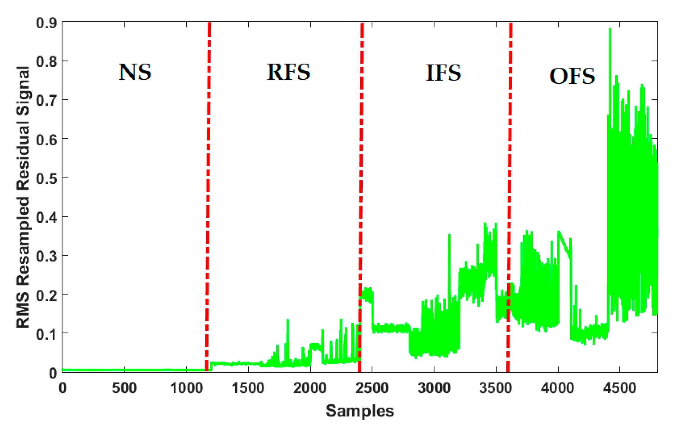
After generating the residual signals for all conditions, the resampled root means square (RMS) residual signals are determined. The resampled RMS residual signal is presented as a following definition.
R M S H R K F ( k ) r m s = 1 M j = 1 M R M S H R K F ( k ) 2
Here, R M S H R K F ( k ) r m s and M denote the resampled RMS value for the residual signal of unknown signals using the proposed digital twin (MS-HRKF) and the number of windows to determine the resampled RMS residual signal, respectively. For each state, the residual signal is made up of 120,000 samples. It was segmented into 100 windows; each window contains 1200 samples. For signal classification, the RMS feature is used for 100 windows. The support vector machine (SVM) is suggested for the RMS resampled residual signal classification. The training set includes 75% and the testing set includes the remaining 25%. The details of the training and testing datasets for FPRCI using SVM are illustrated in Table 3. In addition, Algorithm 1 illustrates the design steps of the proposed scheme.
Algorithm 1 The proposed approach: Intelligent digital twin integrated with SVM for bearing anomaly detection and crack size identification.
1.1. Digital Twin’s Signal ApproximationNo of Eq.
1:Vibration bearing signal approximation using the MAT algorithm.(10)
2:Vibration bearing signal approximation using the AUT technique.(11,12)
3:Improve the robustness in the AUT using the AUT-LAG method.(13,14)
4:Increase the accuracy in the AUT-LAG using the SAL approach.(15,16)
5:Combination of the MAT algorithm and the SAL approach for the proposed approach for vibration bearing signal approximation.(21,22)
1.2. Digital Twin’s Signal Estimation
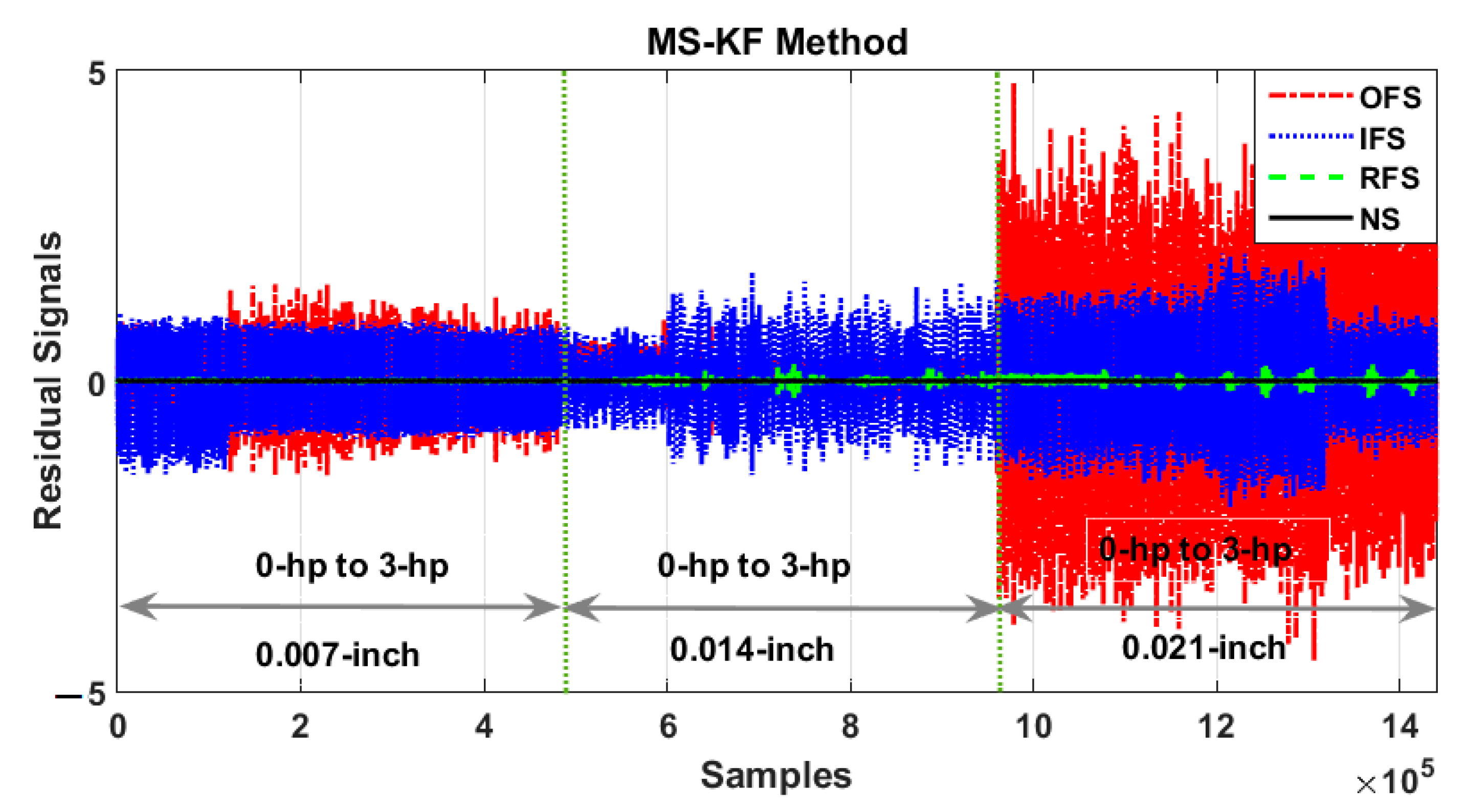
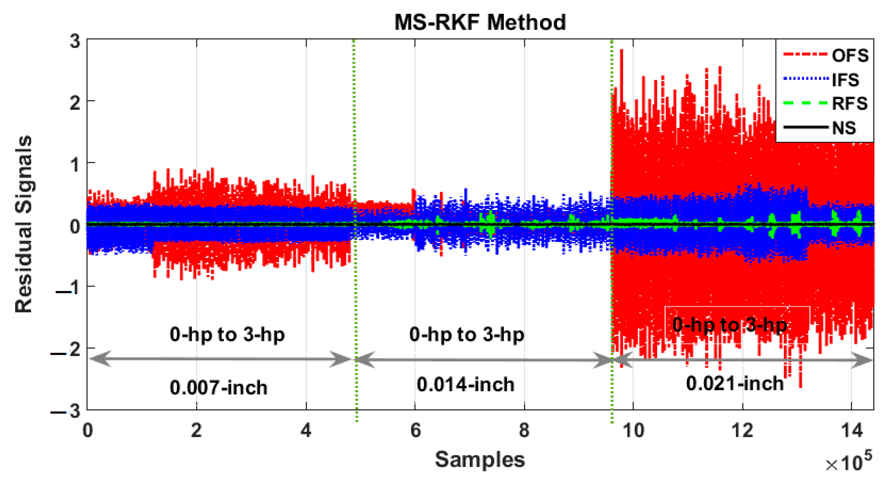
6:Vibration bearing signal estimation using the MS-KF method.(23,25)
7:Increase the robustness in the MS-KF using the MS-RKF approach.(26–30)
6:Increase the accuracy and reliability in the MS-RKF using the MS-HRKF technique.(31–34)
2. Residual Signal Determination
7:Determine the intelligent digital twin (MS-HRKF) residual signal. (38)
3. Signal Classification
8:Resample the residual signals and find the RMS resampled residual signal. (39)
9:Pattern recognition and crack size identification using SVM.

3. Experimental Results and Discussion

To experiment with the power of the proposed scheme for FPRCI, the CWRUD was used in this study. The vibration sensor was selected for data collection. This sensor collects signals in the following four classes: NS, RFS, IFS, and OFS. Moreover, the crack sizes for the RFS, IFS, and OFS are 0.007, 0.014, and 0.021 inch. Furthermore, the motor torque load varies from 0 to 3 hp for all four classes. The experimental results have three main sections: digital twin test and analysis, residual signals assessment and investigation, and classification analysis.

3.1. Digital Twin Test and Analysis

Figure 3 shows the original RAW signal for the bearing for the NS, RFS, IFS, and OFS when the crack sizes are 0.007, 0.014, and 0.021 inch in four different motor torque loads from 0 to 3 hp.
In Figure 3, when the crack sizes are 0.007 inch, the IFS and OFS overlap which can increase the rate of misclassification. Besides, when the crack size is 0.014 inch, the challenge of classification between OFS, IFS, and RFS increases sharply. In addition, when the crack size is 0.21 inch, the challenge of misclassification is increased between RFS and INS. Thus, the original RAW signals cannot be used for the bearing FPRCI. To improve the performance of the bearing FPRCI, in the first step, digital twin-based modeling was recommended in this study. Figure 4 shows the original normal RAW signal and modeled signal using the proposed digital twin signal modeling (MS) scheme. Based on Figure 4, the power of RAW signal modeling using proposed digital twin signal modeling (MS) scheme is very good.
Figure 5 illustrates the bearing modeling in normal conditions using four algorithms: the proposed digital twin signal modeling (MS) scheme, the SAL technique, the AUT-LAG technique, and the AUT method.
Based on Figure 5, the error of normal signal modeling of the bearing for the digital twin using the proposed scheme is less than the others. Thus, the accuracy and robustness of the proposed (MS) digital twin modeling approach is better than the others. Moreover, the covariance power spectral density estimation of the normal signal and the modeled signal using MS technique is illustrated in Figure 6 to describe the distribution of power into the frequency components composing those signals. Regarding this figure, the distribution of the signal’s power into the frequency for normal signal and the estimated normal signal is very close.
Figure 7 and Figure 8 show the bode plot for the original normal signal and modeled normal signal. Regarding these figures, the bode plot for the original normal signal and modeled normal signal are very similar.
To test the power of signal modeling against some external change, impulse response is suggested for original normal signal and modeled normal signal. Figure 9 and Figure 10 illustrate the impulse response for original normal signal and modeled normal signal.

3.2. Residual Signals Test and Analysis

After modeling and estimation, the bearing signals to design a digital twin and the residual signals are computed using the difference between the original (RAW) signals and the estimated signals. To test the effectiveness of the proposed digital twin estimation technique (MS-HRKF), this technique is compared with the following algorithms: (a) the MS-KF and (b) the MS-RKF. According to Equations (23) and (26), the residual signals for the MS-KF technique, ( R M S K F ( k ) ) , and MS-RKF technique, ( R M S R K F ( k ) ) , are computed as the following equations, respectively.
R M S K F ( k ) = Z ( k ) Z M S K F ( k )
R M S R K F ( k ) = Z ( k ) Z M S R K F ( k )
Figure 11 shows the power of the MS-KF for the classification condition of the CWRUD bearing signals in diverse situations.
Regarding the comparison between Figure 3 and Figure 11, it can be seen that the MS-KF improves the classification. Moreover, Figure 12 shows the power of the MS-RKF for the classification condition of the bearing signals in different conditions. Regarding the comparison between Figure 3 and Figure 12, it can be seen that the MS-RKF improves the classification. Regarding Figure 3, the CWRUD for the bearing has a significant challenge in classification, especially when the crack sizes are 0.007 and 0.014 inch. The MS-RKF improves the classification’s accuracy, especially when the crack size is 0.007 inch. Figure 13 illustrates the residual signals of the proposed digital twin (MS-HRKF) method. Regarding Figure 13, the overlapping and misclassification of the residual signals in the proposed digital twin (MS-HRKF) are reduced sharply.
Regarding this figure, the proposed digital twin (MS-HRKF) method improves the detection and identification of the fault crack sizes sharply. According to the comparison between Figure 12 and Figure 13, it is clear that the MS-RKF has a serious challenge for classification when the crack size is 0.014 inch. The proposed digital twin (MS-HRKF) solves this problem. Thus, based on Figure 11, Figure 12 and Figure 13, the accuracy of the proposed digital twin (MS-HRKF) for the CWRUD for bearing signal classification is better than the MS-RKF and the MS-KF. In addition, the power spectral density estimation for NS, RFS, IFS, and OFS using proposed method is illustrated in Figure 14 to describe the distribution of power into the frequency components composing those signals. Regarding this figure, the distribution of the signal’s power into the frequency for NS, RFS, IFS, and OFS are separable.
Figure 15 shows the RMS residual signal using proposed digital twin (MS-HRKF) method. Based on this technique, it is clear that the signal is easy to classify.

3.3. Classification Analysis

To test the power of the proposed method for FPRCI, the combination of the proposed digital twin integrated with the SVM (hence called MS-HRKF+SVM) is compared with the combination of the MS-RKF with SVM (hence called MS-RKF+SVM) and the combination of the MS-KF with SVM (hence called MS-KF+SVM). Figure 16, Figure 17 and Figure 18 illustrate the confusion matrices for 10 experiments to show the accuracy of the fault pattern recognition (FPR) in the proposed digital twin integrated with SVM (MS-HRKF+SVM), the MS-RKF+SVM, and the MS-KF+SVM. In the combination of the MS-KF with SVM, the nonlinear signal modeling algorithm is integrated with the linear estimation algorithm. This algorithm has two important challenges: linear estimator and robustness. To improve the robustness the combination of the MS-RKF with SVM is recommended.
Based on Figure 17 and Figure 18, the combination of the MS-RKF with SVM improves the accuracy of FPR in the combination of the MS-KF with SVM by around 4.9%. To solve the challenge of the linear estimator in the combination of the MS-RKF with SVM and the combination of the MS-RKF with SVM, the proposed digital twin integrated with SVM (MS-HRKF+SVM) is suggested. Based on these figures, the average FPR in the proposed digital twin integrated with SVM (MS-HRKF+SVM), the combination of the MS-RKF with SVM, and the combination of the MS-KF with SVM, respectively, are 99.5%, 87%, and 82.1%. Thus, the proposed digital twin integrated with SVM (MS-HRKF+SVM) improves the accuracy of FPR in the combination of the MS-RKF with SVM and the combination of the MS-KF with SVM by 12.55% and 17.4%, respectively.
Moreover, Figure 19 shows the impact of the robustness in the proposed digital twin integrated with SVM (MS-HRKF+SVM), the combination of the MS-RKF with SVM, and the combination of the MS-KF with SVM for 10 experiments.
Based on Figure 19, due to the boxplot, the resistance of the proposed digital twin integrated with SVM (MS-HRKF+SVM) is higher than the others. Regarding this figure, the impact of the high-order variable structure technique (HVS) is clear in the proposed digital twin integrated with SVM (MS-HRKF+SVM) and the combination of the MS-RKF with SVM compared to the combination of the MS-KF with SVM.
Table 4, Table 5 and Table 6 demonstrate the power of the proposed digital twin integrated with SVM (MS-HRKF+SVM), the combination of the MS-RKF with SVM (MS-RKF+SVM), and the combination of the MS-KF with SVM (MS-KF+SVM) for crack size identification (CSI). Table 4 shows the impact of the proposed digital twin integrated with SVM (MS-HRKF+SVM), the combination of the MS-RKF with SVM, and the combination of the MS-KF with SVM for the ball CSI when the crack sizes are 0.007, 0.014, and 0.021 inch. Based on this table, the average ball CSI accuracies are 98.7%, 88.9%, and 77.7%, respectively, using the proposed digital twin integrated with SVM (MS-HRKF+SVM), the combination of the MS-RKF with SVM, and combination of the MS-KF with SVM. Thus, the proposed digital twin integrated with SVM (MS-HRKF+SVM) improves the average ball CSI in the combination of the MS-RKF with SVM and the combination of the MS-KF with SVM by 9.8% and 21%, respectively.
Table 5 illustrates the impact of the proposed digital twin integrated with SVM (MS-HRKF+SVM), the combination of the MS-RKF with SVM, and the combination of the MS-KF with SVM for the inner CSI when the crack sizes are 0.007, 0.014, and 0.021 inch. Based on this table, the average inner CSI accuracies are 100%, 90.1%, and 77.7%, respectively, using the proposed digital twin integrated with SVM (MS-HRKF+SVM), the combination of the MS-RKF with SVM, and the combination of the MS-KF with SVM. Hence, the proposed digital twin integrated with SVM (MS-HRKF+SVM) improves the average inner CSI in the combination of the MS-RKF with SVM and the combination of the MS-KF with SVM by 9.9% and 22.3%, respectively. Table 6 proves the effect of the proposed digital twin integrated with SVM (MS-HRKF+SVM), the combination of the MS-RKF with SVM, and the combination of the MS-KF with SVM for the outer CSI when the crack sizes are 0.007, 0.014, and 0.021 inch. Based on this table, the average outer CSI accuracies are 100%, 90.7%, and 80.8%, respectively, using the proposed digital twin integrated with SVM (MS-HRKF+SVM), the combination of the MS-RKF with SVM, and the combination of the MS-KF with SVM. Henceforth, the proposed digital twin integrated with SVM (MS-HRKF+SVM) modifies the average outer CSI in the combination of the MS-RKF with SVM and the combination of the MS-KF with SVM by 9.3% and 19.2%, respectively.
Based on Table 4, Table 5 and Table 6, the power of the CSI in the proposed digital twin integrated with SVM (MS-HRKF+SVM) is better than the other two methods. Thus, the proposed digital twin integrated with SVM (MS-HRKF+SVM) is more reliable than the other two methods for the ball, inner, and outer CSI. Furthermore, Figure 12 demonstrates the effect of the robustness in the proposed digital twin integrated with SVM (MS-HRKF+SVM), the combination of the MS-RKF with SVM, and the combination of the MS-KF with SVM for 10 experiments. Based on this figure, due to the boxplot, the resistance of the proposed digital twin integrated with SVM (MS-HRKF+SVM) for the outer, inner, and ball CSI is better than the other two approaches. Thus, based on Figure 8, Figure 9 and Figure 10, the accuracy of the proposed digital twin integrated with SVM (MS-HRKF+SVM) is significantly better than the combination of the MS-RKF with SVM and the combination of the MS-KF with SVM for bearing FPR. In addition, based on Figure 11, the proposed digital twin integrated with SVM (MS-HRKF+SVM) is more robust than the combination of the MS-RKF with SVM and the combination of the MS-KF with SVM for bearing FPR. Table 4, Table 5 and Table 6 and Figure 20 show that the impact (accuracy and robustness) of the proposed digital twin integrated with SVM (MS-HRKF+SVM) for the bearing CSI is better than the combination of the MS-RKF with SVM and the combination of the MS-KF with SVM.

4. Conclusions

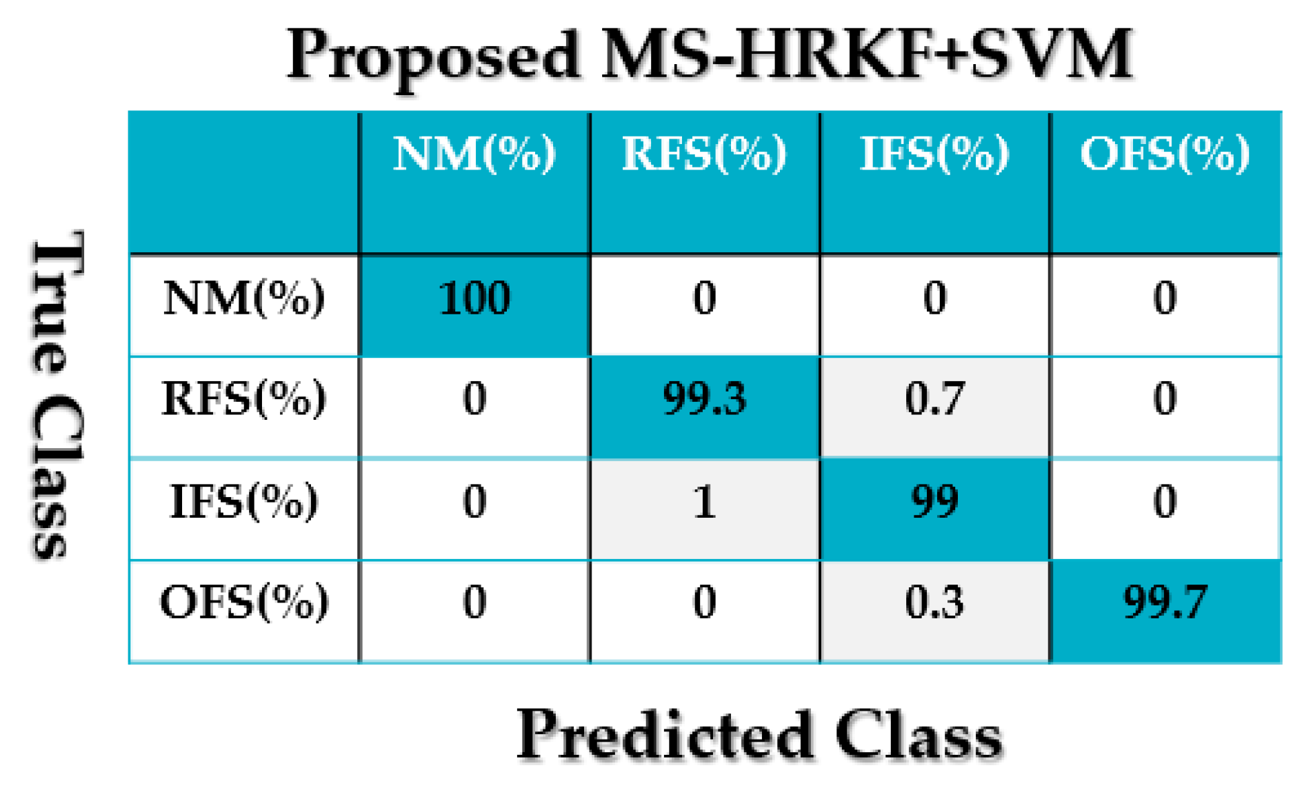
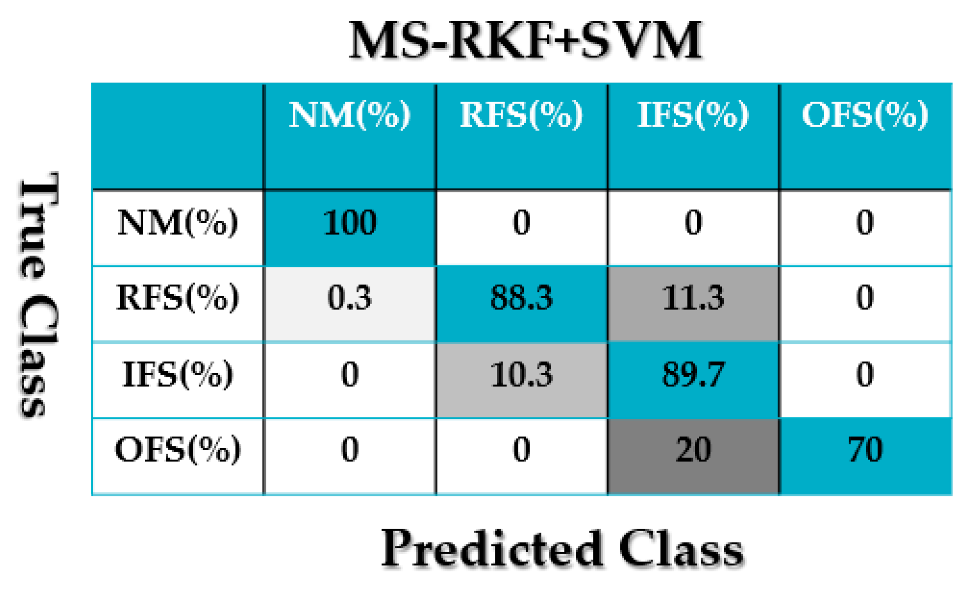
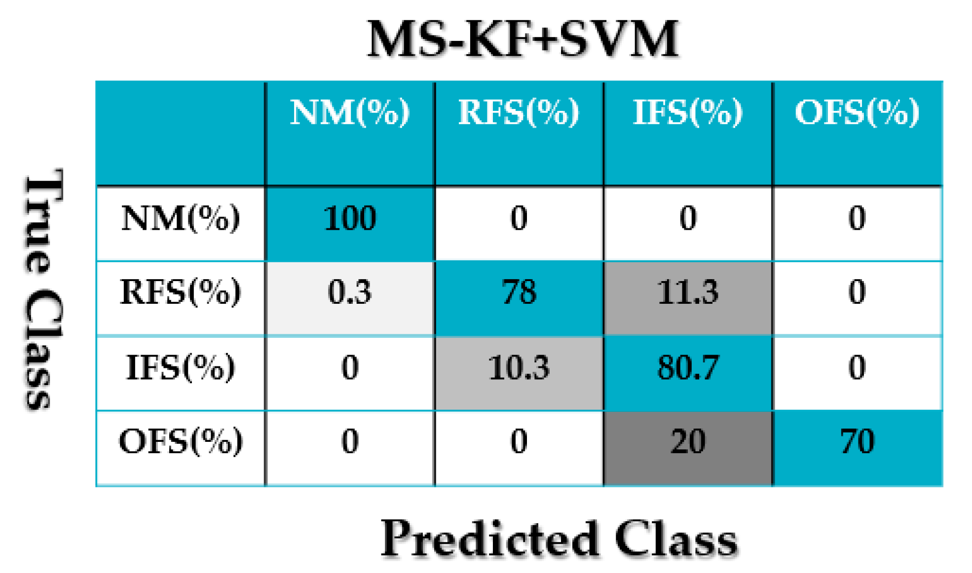
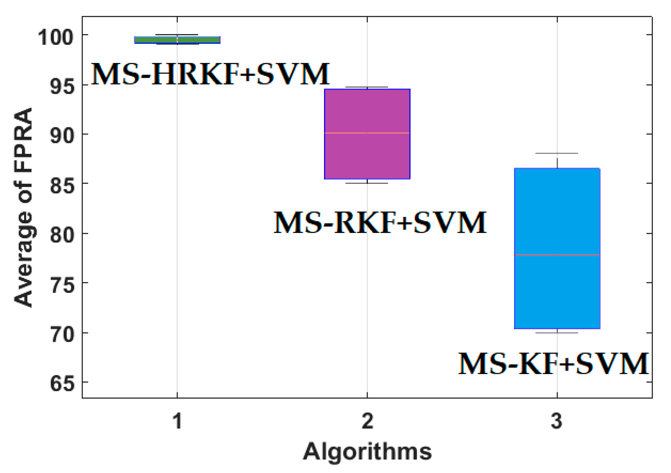
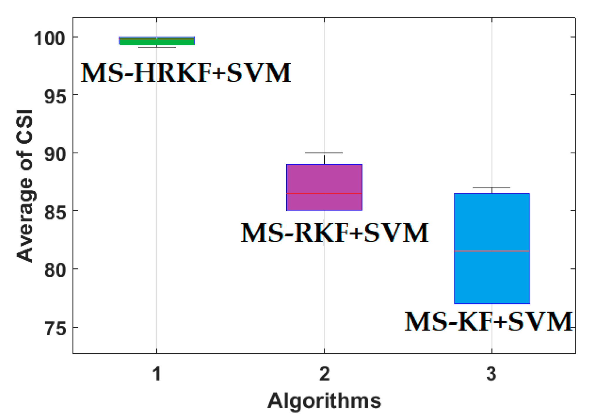
In this research, the application of the intelligent digital twin integrated with machine learning was observed for bearing anomaly detection and crack size identification. The proposed algorithm had three main parts: intelligent digital twin, residual signal determination, and anomaly classification, and crack size identification. The first part of the intelligent digital twin was the function approximator. The integration of the mathematical-based vibration signal modeling, autoregressive with Laguerre technique, and support vector regression was recommended for the proposed function approximator. Moreover, the next part of the intelligent digital twin was the signal estimator. The combination of a Kalman filter, the high-order variable structure technique, and the adaptive neural-fuzzy approach was used for signal estimation. After designing the intelligent digital twin, the residual signals were determined. The residual signals were resampled and the RMS feature was extracted from the resampled residual signals. In the final stage of design, the SVM was integrated with an intelligent digital twin to identify the bearing crack sizes and fault patterns. The impact of the proposed scheme was tested by CWRUBD and compared with the MS-RKF and the MS-KF algorithms. Regarding the experimental results, the proposed scheme improved the average accuracy for the bearing fault pattern recognition by 12.55% and 17.4%, respectively, compared with the MS-RKF and the MS-KF algorithms. In addition, in the view of crack size identification, the impact of the proposed technique was 98.7%, 100%, and 100% for the ball, inner, and outer faults, respectively. For future work, the parallel machine/deep learning digital twin will be suggested for fault diagnosis of nonlinear systems with nonstationary signals.

Author Contributions

Conceptualization, F.P. and J.-M.K.; data curation, F.P.; formal analysis, F.P. and J.-M.K.; funding acquisition, J.-M.K.; methodology, F.P. and J.-M.K.; software, F.P.; supervision, J.-M.K.; validation, F.P. and J.-M.K.; visualization, F.P. and J.-M.K.; writing—original draft, F.P.; writing—review and editing, F.P. and J.-M.K. All authors have read and agreed to the published version of the manuscript.

Funding

This work was supported by 2021 Research Fund of University of Ulsan.

Data Availability Statement

The data are publicly available.

Conflicts of Interest

The authors declare no conflict of interest.

References

  1. Sihag, N.; Sangwan, K.S. A systematic literature review on machine tool energy consumption. J. Clean. Prod. 2020, 275, 123125. [Google Scholar] [CrossRef]
  2. Huayu, Z.; Zhang, C.; Wang, C.; Xie, F. A survey of non-destructive techniques used for inspection of bearing steel balls. Measurement 2020, 159, 107773. [Google Scholar]
  3. Subhasis, N.; Toliyat, H.A.; Li, X. Condition monitoring and fault diagnosis of electrical motors—A review. IEEE Trans. Energy Convers. 2005, 20, 719–729. [Google Scholar]
  4. Liu, Z.; Zhang, L. A review of failure modes, condition monitoring and fault diagnosis methods for large-scale wind turbine bearings. Measurement 2020, 149, 107002. [Google Scholar] [CrossRef]
  5. He, M.; He, D. A new hybrid deep signal processing approach for bearing fault diagnosis using vibration signals. Neurocomputing 2020, 396, 542–555. [Google Scholar] [CrossRef]
  6. Xu, Y.; Zhen, D.; Gu, J.X.; Rabeyee, K.; Chu, F.; Gu, F.; Ball, A.D. Autocorrelated Envelopes for early fault detection of rolling bearings. Mech. Syst. Signal Process. 2021, 146, 106990. [Google Scholar] [CrossRef]
  7. Qin, Y. A new family of model-based impulsive wavelets and their sparse representation for rolling bearing fault diagnosis. IEEE Trans. Ind. Electron. 2017, 65, 2716–2726. [Google Scholar] [CrossRef]
  8. Zhao, B.; Yuan, Q.; Zhang, H. An improved scheme for Vibration-Based rolling bearing fault diagnosis using feature integration and AdaBoost tree-based ensemble classifier. Appl. Sci. 2020, 10, 1802. [Google Scholar] [CrossRef] [Green Version]
  9. Wihan, B.; Wilke, D.N.; Heyns, S. Deep digital twins for detection, diagnostics and prognostics. Mech. Syst. Signal Process. 2020, 140, 106612. [Google Scholar]
  10. Farzin, P.; Kim, J.-M. Bearing fault diagnosis by a robust higher-order super-twisting sliding mode observer. Sensors 2018, 18, 1128. [Google Scholar]
  11. Parker, R.G.; Guo, Y.; Eritenel, T.; Ericson, T.M. Vibration Propagation of Gear Dynamics in a Gear-Bearing-Housing System Using Mathematical Modeling and Finite Element Analysis; NASA Glenn Research Center: Cleveland, OH, USA, 2012. [Google Scholar]
  12. Prakash, G. A Bayesian approach to degradation modeling and reliability assessment of rolling element bearing. Commun. Stat. Theory Methods 2020, 1–22. [Google Scholar] [CrossRef]
  13. Antoni, J.; Bonnardot, F.; Raad, A.; El Badaoui, M. Cyclostationary modelling of rotating machine vibration signals. Mech. Syst. Signal Process. 2004, 18, 1285–1314. [Google Scholar] [CrossRef]
  14. Kumbhar, S.G. An integrated approach of Adaptive Neuro-Fuzzy Inference System and dimension theory for diagnosis of rolling element bearing. Measurement 2020, 166, 108266. [Google Scholar] [CrossRef]
  15. Rahmoune, M.B.; Hafaifa, A.; Kouzou, A.; Chen, X.; Chaibet, A. Gas turbine monitoring using neural network dynamic nonlinear autoregressive with external exogenous input modelling. Math. Comput. Simul. 2021, 179, 23–47. [Google Scholar] [CrossRef]
  16. Yang, H.; Rad, H.N.; Hasanipanah, M.; Amnieh, H.B.; Nekouie, A. Prediction of vibration velocity generated in mine blasting using support vector regression improved by optimization algorithms. Nat. Resour. Res. 2020, 29, 807–830. [Google Scholar] [CrossRef]
  17. Cheng, C.; Ma, G.; Zhang, Y.; Sun, M.; Teng, F.; Ding, H.; Yuan, Y. A deep learning-based remaining useful life prediction approach for bearings. IEEE ASME Trans. Mechatron. 2020, 25, 1243–1254. [Google Scholar] [CrossRef] [Green Version]
  18. Chen, L.; Xu, G.; Zhang, S.; Yan, W.; Wu, Q. Health indicator construction of machinery based on end-to-end trainable convolution recurrent neural networks. J. Manuf. Syst. 2020, 54, 1–11. [Google Scholar] [CrossRef]
  19. Gao, Y.; Liu, X.; Xiang, J. FEM simulation-based generative adversarial networks to detect bearing faults. IEEE Trans. Ind. Inform. 2020, 16, 4961–4971. [Google Scholar] [CrossRef]
  20. Alia, S.; Nasri, R.; Meddour, I.; Younes, R. Comparison between sound perception and self-organizing maps in the monitoring of the bearing degradation. Int. J. Adv. Manuf. Technol. 2020, 110, 2003–2013. [Google Scholar] [CrossRef]
  21. Pan, T.; Chen, J.; Pan, J.; Zhou, Z. A deep learning network via shunt-wound restricted Boltzmann machines using raw data for fault detection. IEEE Trans. Instrum. Meas. 2019, 69, 4852–4862. [Google Scholar] [CrossRef]
  22. Dai, W.; Mo, Z.; Luo, C.; Jiang, J.; Zhang, H.; Miao, Q. Fault diagnosis of rotating machinery based on deep reinforcement learning and reciprocal of smoothness index. IEEE Sens. J. 2020, 20, 8307–8315. [Google Scholar] [CrossRef]
  23. Kong, X.; Mao, G.; Wang, Q.; Ma, H.; Yang, W. A multi-ensemble method based on deep auto-encoders for fault diagnosis of rolling bearings. Measurement 2020, 151, 107132. [Google Scholar] [CrossRef]
  24. Stack, J.R.; Habetler, T.G.; Harley, R.G. Bearing fault detection via autoregressive stator current modeling. IEEE Trans. Ind. Appl. 2004, 40, 740–747. [Google Scholar] [CrossRef]
  25. Abid, A.; Khan, M.T.; Iqbal, J. A review on fault detection and diagnosis techniques: Basics and beyond. Artif. Intell. Rev. 2020, 10, 1–26. [Google Scholar] [CrossRef]
  26. Piltan, F.; Kim, J.-M. Bearing fault identification using machine learning and adaptive cascade fault observer. Appl. Sci. 2020, 10, 5827. [Google Scholar] [CrossRef]
  27. TayebiHaghighi, S.; Koo, I. Fault diagnosis of rotating machine using an indirect observer and machine learning. In Proceedings of the 2020 International Conference on Information and Communication Technology Convergence (ICTC), Jeju, Korea, 21–23 October 2020; pp. 277–282. [Google Scholar]
  28. Gou, L.; Shen, Y.; Zheng, H.; Zeng, X. Multi-Fault diagnosis of an aero-engine control system using joint sliding mode observers. IEEE Access 2020, 8, 10186–10197. [Google Scholar] [CrossRef]
  29. Meng, X.; Yu, H.; Xu, T.; Wu, H. Disturbance observer and l2-gain-based state error feedback linearization control for the quadruple-tank liquid-level system. Energies 2020, 13, 5500. [Google Scholar] [CrossRef]
  30. Piltan, F.; Prosvirin, A.E.; Sohaib, M.; Saldivar, B.; Kim, J.-M. An SVM-based neural adaptive variable structure observer for fault diagnosis and fault-tolerant control of a robot manipulator. Appl. Sci. 2020, 10, 1344. [Google Scholar] [CrossRef] [Green Version]
  31. Islam, S.I.; Lim, C.-C.; Shi, P. Robust fault detection of TS fuzzy systems with time-delay using fuzzy functional observer. Fuzzy Sets Syst. 2020, 392, 1–23. [Google Scholar] [CrossRef]
  32. Guo, X.-G.; Tian, M.-E.; Li, Q.; Ahn, C.K.; Yang, Y.-H. Multiple-fault diagnosis for spacecraft attitude control systems using RBFNN-based observers. Aerosp. Sci. Technol. 2020, 106, 106195. [Google Scholar] [CrossRef]
  33. Guzman, J.; López-Estrada, F.R.; Estrada-Manzo, V.; Valencia-Palomo, G. Actuator fault estimation based on a proportional-integral observer with nonquadratic Lyapunov functions. Int. J. Syst. Sci. 2021, 1–14. [Google Scholar] [CrossRef]
  34. Hu, J.; Zheng, S.; Liu, X.; Wang, M.; Deng, J.; Yan, F. Optimizing the fault diagnosis and fault-tolerant control of selective catalytic reduction hydrothermal aging using the Unscented Kalman Filter observer. Fuel 2021, 288, 119827. [Google Scholar] [CrossRef]
  35. Krokavec, D.; Filasová, A. Discrete-time linear systems fault diagnosis using schmidt-kalman filters. In Proceedings of the 2020 21th International Carpathian Control Conference (ICCC), High Tatras, Slovakia, 27–29 October 2020; pp. 1–6. [Google Scholar]
  36. Wang, Z.; Yao, L.; Cai, Y. Rolling bearing fault diagnosis using generalized refined composite multiscale sample entropy and optimized support vector machine. Measurement 2020, 156, 107574. [Google Scholar] [CrossRef]
  37. Castellanos, M.B.; Serpa, A.L.; Biazussi, J.L.; Verde, W.M.; Sassim, N.D.S.D.A. Fault identification using a chain of decision trees in an electrical submersible pump operating in a liquid-gas flow. J. Pet. Sci. Eng. 2020, 184, 106490. [Google Scholar] [CrossRef]
  38. Li, Y.; Sarvi, M.; Khoshelham, K.; Haghani, M. Multi-view crowd congestion monitoring system based on an ensemble of convolutional neural network classifiers. J. Intell. Transp. Syst. 2020, 24, 437–448. [Google Scholar] [CrossRef]
  39. Pulgar, F.J.; Charte, F.; Rivera, A.J.; del Jesus, M.J. Choosing the proper autoencoder for feature fusion based on data complexity and classifiers: Analysis, tips and guidelines. Inf. Fusion 2020, 54, 44–60. [Google Scholar] [CrossRef]
  40. Bearing Data Center. Case Western Reserve University Seeded Fault Test Data. Available online: https://csegroups.case.edu/bearingdatacenter/pages/welcome-case-western-reserve-university-bearing-data-center-website (accessed on 23 December 2020).
  41. Mishra, C.; Samantaray, A.K.; Chakraborty, G. Ball bearing defect models: A study of simulated and experimental fault signatures. J. Sound Vib. 2017, 400, 86–112. [Google Scholar] [CrossRef]
  42. Njima, B.; Garna, T. PIO output fault diagnosis by ARX-Laguerre model applied to 2nd order electrical system. IEEE Access 2020, 8, 83052–83061. [Google Scholar] [CrossRef]
Figure 1. Proposed intelligent digital twin integrated with machine learning for bearing anomaly classification.
Applsci 11 04602 g001
Figure 2. Experimental testbed for the bearing data acquisition implemented by CWRUBD [10,40].
Applsci 11 04602 g002
Figure 3. The CWRUD bearing vibration signals for NS, RFS, IFS, and OFS when the motor torque loads vary from 0 to 3 hp; moreover, the crack sizes for abnormal conditions are 0.007, 0.014, and 0.021 inch.
Applsci 11 04602 g003
Figure 4. The original normal RAW signal and the modeled signal using proposed (MS) scheme.
Applsci 11 04602 g004
Figure 5. The error of the bearing normal signal modeling for the digital twin using four algorithms: AUT method, AUT-LAG technique, SAL approach, and proposed (MS) scheme.
Applsci 11 04602 g005
Figure 6. The frequency response of original normal signal and modeled normal signal using covariance power spectral density estimation.
Applsci 11 04602 g006
Figure 7. Bode plot for original normal signal.
Applsci 11 04602 g007
Figure 8. Bode plot for modeled normal signal.
Applsci 11 04602 g008
Figure 9. Impulse response estimated plot for original normal signal.
Applsci 11 04602 g009
Figure 10. Impulse response estimated plot for modeled normal signal.
Applsci 11 04602 g010
Figure 11. The residual signals of the bearing using the MS-KF algorithm when the motor torque loads vary from 0 to 3 hp; moreover, the crack sizes for abnormal conditions are 0.007, 0.014, and 0.021 inch.
Applsci 11 04602 g011
Figure 12. The residual signals of the bearing using the MS-RKF algorithm when the motor torque loads vary from 0 to 3 hp; moreover, the crack sizes for abnormal conditions are 0.007, 0.014, and 0.021 inch.
Applsci 11 04602 g012
Figure 13. The residual signals of the bearing using the proposed digital twin (MS-HRKF) algorithm when the motor torque loads vary from 0 to 3 hp; moreover, the crack sizes for abnormal conditions are 0.007, 0.014, and 0.021 inch: (a) all cases and (b) zoom view for NS and RFS.
Applsci 11 04602 g013
Figure 14. The frequency response of power spectral density estimation for NS, RFS, IFS, and OFS using the proposed method.
Applsci 11 04602 g014
Figure 15. RMS resampled residual signal using the proposed digital twin (MS-HRKF) algorithm when the motor torque loads vary from 0 to 3 hp; moreover, the crack sizes for abnormal conditions are 0.007, 0.014, and 0.021 inch.
Applsci 11 04602 g015
Figure 16. Confusion matrices for FPR using the proposed digital twin integrated with the SVM (MS-HRKF+SVM) technique.
Applsci 11 04602 g016
Figure 17. Confusion matrices for FPR using the combination of the MS-RKF with SVM (MS-RKF+SVM) technique.
Applsci 11 04602 g017
Figure 18. Confusion matrices for FPR using the combination of the MS-KF with SVM (MS-KF+SVM) technique.
Applsci 11 04602 g018
Figure 19. Boxplots of the average FPRA metrics over 10 experiments for the proposed digital twin integrated with SVM (MS-HRKF+SVM), the MS-RKF+SVM, and the MS-KF+SVM to test the power of robustness.
Applsci 11 04602 g019
Figure 20. Boxplots of the average CSI metrics over 10 experiments for the MS-HRKF+SVM, the MS-RKF+SVM, and the MS-KF+SVM to test the power of robustness.
Applsci 11 04602 g020
Table 1. Summarized information of the CWRUBD [40].
Dataset GroupStatesLoad (hp)Crack Sizes (inch)
iNS00.007, 0.014, and 0.021
RFS0
IFS0
OFS0
iiNS10.007, 0.014, and 0.021
RFS1
IFS1
OFS1
iiiNS20.007, 0.014, and 0.021
RFS2
IFS2
OFS2
ivNS30.007, 0.014, and 0.021
RFS3
IFS3
OFS3
Table 2. Information of the bearing for mathematical modeling of the CWRUBD [10,40].
ParametersValue
Number of rollers 9
Stiffness of roller 5.96 × 10 7   ( N m )
Mass of outer (kg) 2.7   ( Kg )
Stiffness of outer 1.31 × 10 5   ( N m )
Mass of shaft (kg) 1.36   ( Kg )
Stiffness of shaft 23.3 × 10 6   ( N m )
Damping 654   ( NS m )
Roller diameter 7.940   ( mm )
Pitch diameter 39.04   ( mm )
Defect size 7   ( mm )
Defect depth 2   ( mm )
Inside diameter25 (mm)
Outside diameter52 (mm)
Ball diameter7.94 (mm)
Thickness15 (mm)
Table 3. Details of the training and testing resampled RMS residual signals using SVM.
Training SamplesTesting Samples
Pattern recognitionNS900300
RFS900300
IFS900300
OFS900300
Crack size identificationRFS0.007 inch300100
0.014 inch300100
0.021 inch300100
IFS0.007 inch300100
0.014 inch300100
0.021 inch300100
OFS0.007 inch300100
0.014 inch300100
0.021 inch300100
Table 4. Average accuracy of the ball CSI using the proposed MS-HRKF+SVM, the MS-RKF+SVM, and the MS-KF+SVM.
Ball Crack Sizes (inch)0.0070.0140.021Average
MS-HRKF+SVM (%) 100979998.7
MS-RKF+SVM (%)88.882.595.588.9
MS-KF+SVM (%)78.27381.877.7
Table 5. Average accuracy of the inner CSI using the proposed MS-HRKF+SVM, the MS-RKF+SVM, and the MS-KF+SVM.
Inner Crack Sizes (inch)0.0070.0140.021Average
MS-HRKF+SVM (%) 100100100100
MS-RKF+SVM (%)9088.891.590.1
MS-KF+SVM (%)70.27884.877.7
Table 6. Average accuracy of the outer CSI using the proposed MS-HRKF+SVM, the MS-RKF+SVM, and the MS-KF+SVM.
Outer Crack Sizes (inch)0.0070.0140.021Average
MS-HRKF+SVM (%) 100100100100
MS-RKF+SVM (%)9583.893.590.7
MS-KF+SVM (%)77.38085.380.8
Publisher’s Note: MDPI stays neutral with regard to jurisdictional claims in published maps and institutional affiliations.

