Traffic Monitoring System Based on Deep Learning and Seismometer Data

Abstract

Currently, vehicle classification in roadway-based techniques depends mainly on photos/videos collected by an over-roadway camera or on the magnetic characteristics of vehicles. However, camera-based techniques are criticized for potentially violating the privacy of vehicle occupants and exposing their identity, and vehicles can evade detection when they are obscured by larger vehicles. Here, we evaluate methods of identifying and classifying vehicles on the basis of seismic data. Vehicle identification from seismic signals is considered a difficult task because of interference by various noise. By analogy with techniques used in speech recognition, we used different artificial intelligence techniques to extract features of three, different-sized vehicles (buses, cars, motorcycles) and seismic noise. We investigated the application of a deep neural network (DNN), a convolutional neural network (CNN), and a recurrent neural network (RNN) to classify vehicles on the basis of vertical-component seismic data recorded by geophones. The neural networks were trained on 5580 unprocessed seismic records and achieved excellent training accuracy (99%). They were also tested on large datasets representing periods as long as 1 month to check their stability. We found that CNN was the most satisfactory approach, reaching 96% accuracy and detecting multiple vehicle classes at the same time at a low computational cost. Our findings show that seismic methods can be used for traffic monitoring and security purposes without violating the privacy of vehicle occupants, offering greater efficiency and lower costs than current methods. A similar approach may be useful for other types of transportation, such as vessels and airplanes.

1. Introduction

Many countries invest heavily in traffic monitoring systems [1], which collect and analyze traffic data to derive statistical information, such as the numbers of vehicles on the road and their temporal patterns. Governments use these statistics to forecast transportation needs, improve transportation safety, and schedule pavement maintenance work. Identifying the size of vehicles is a key task that helps to predict noise levels and road damage. The characteristic mix of vehicle types that use a roadway can determine the geometric design of the road based on the Traffic Monitoring Guide report published by the Federal Highway Administration in the United States [2].

Vehicle classification systems make use of many recent advances in sensing and machine learning technologies [3]. Although newer systems perform vehicle classification with higher accuracy, they differ in their characteristics and requirements, such as the types of sensors used, parameter settings, operating environment, and cost. Many traffic monitoring systems rely on vision-based vehicle classification techniques, usually based on cameras, that deliver high classification accuracy ranged between 90%~99% [4], covering large areas compared with emerging alternatives. Although camera-based systems have high classification accuracy, their performance can be affected by weather and lighting conditions as well as other factors. For instance, vehicles can be missed when they are obscured by large vehicles. Furthermore, the system requires huge investments in infrastructures to perform a complete coverage of the road network. Another important problem is the privacy concerns of vehicle occupants, as many people do not feel comfortable being exposed to cameras. An inductive loop detector based on magnetic characteristics of vehicles is one of the most commonly used traffic monitoring systems for vehicle detection and classification [5]. The loop detector system is based on a coil of wire placed under the roadway to capture the change in the magnetic profile signal’s characteristics, such as amplitude, phase, and frequency, when a vehicle passes over it [6]. Several studies on the loop detector technique have shown its high accuracy (99% accuracy) for large vehicle classification, such as cars, trucks, and vans [7,8,9,10], it was also proven that loop detectors have no dependency on the vehicle speed [11]. Although the loop detector system is the most widely adopted in-roadway-based vehicle classification technique, it might not be the most suitable system for easy and low-cost implementation, as it requires coil installation under the roadway surface.

Various privacy-preserving solutions have been proposed, using different kinds of sensors in, over or at the side of roadways [4]. A combination of infrared and ultrasonic sensors (up to 99% accuracy) [12] or magnetic sensors used in roadways and on the side of roadways with accuracy up to 96.4% in the case of using multiple sensor networks [13,14,15]. In addition to previous methods, new methods for traffic congestion monitoring in urban areas were proposed based on GPS, social media data, and network data collected directly from vehicles [16,17,18,19,20]. These methods have contributed to evolving intelligent transport systems (ITSs) and proved clear information of traffic flow and traffic destiny for urban areas. However, most proposed methods have not achieved a classification accuracy comparable to inductive loops and camera-based systems; moreover, they may require special installations, such as loop detectors in the road [21]. Various vibration-based vehicle classification systems have been developed to avoid these shortcomings. Vehicles produce vibrations from two main sources, the engine system and the interaction between the tires and the road [22,23,24]. These signals depend strongly on the size of the vehicle. However, these signals can be hard to identify owing to the complexities of the seismic waveform and the influence of the underlying geology on the propagation of the seismic wave. We have overcome these problems by using artificial intelligence (AI) techniques. Moreover, seismic data are relatively smaller in size than videos recorded by a camera. One hour of a single-channel seismic record is 5 MB, while one hour of video can be 1 GB. For long-term monitoring, smaller data size has a large advantage in data management.

In practice, seismic signals generated by vehicles are hard to distinguish, as most civilian vehicles generate similar vibrations at frequencies below 20 Hz. However, because these signals travel through the ground, they are less sensitive to wind noise, which is an advantage for vehicle detection [25]. Because AI has been instrumental in the dramatic improvement of voice recognition technology in the last decade, such as voice analysis [26], we chose to test the application of similar techniques to recognize vehicles from seismic waves. Furthermore, AI has been widely applied for the classification of seismic events [27,28,29,30]. The application of AI to seismic information for monitoring traffic promises to offer the advantages of low power requirements, easy implementation, and low cost in addition to its advantages in occupant privacy.

A study published in 2010 used a neural network to classify vehicles on the basis of seismic data [31]. The study used acoustic data recorded with a microphone to supplement the seismic data, and the best classification accuracy achieved was 92%. Another study published in 2019 relied exclusively on seismic signatures [25]. That study proposed extracting spectral features of vehicle seismic signals, using a log-scaled frequency cepstral coefficient (LFCC) matrix, a step that requires preprocessing the seismic data in the frequency domain. This method achieved classification accuracy as high as 91.39%. However, both studies concerned heavy military vehicles and cannot be generalized to civilian vehicles. Moreover, both approaches could not use raw seismic data without preprocessing or supplementation by other data.

This paper describes our proposed traffic monitoring system for civilian applications. Our purpose was to build and optimize a neural network that takes a window of waveform data as input, labels it as either seismic noise or a vehicle signal, and identifies the type of vehicle. The proposed approach relies on seismic data alone without preprocessing. In this study, we tested three different neural network architectures that are widely used for the analysis of time series data, including voice recognition. Our approach was applied to civilian traffic and achieved 99% classification accuracy in the training process and 96% accuracy in the validation process.

2. Methods

Neural networks, the main backbone for machine learning, operate in a way that is analogous to biological processes in that the connectivity pattern between neurons resembles the organization of the animal visual cortex [32]. Neural networks use little preprocessing compared to other classification algorithms. This means that the network learns its optimal processing filters, which are manually prepared in traditional algorithms. This independence from prior knowledge and human effort in feature design is a major advantage. Consequently, neural networks can efficiently find relationships between a set of input raw data (in this case, seismic waveforms) and the desired output value (vehicle class probabilities).

Neural networks consist of three main components: neurons, weights, and bias. In a feedforward process, the neurons are determined by the values of the previous input and the weights variable that connect previous inputs to the neuron as shown in Figure 1. Bias is an independent variable that acts as a refresher that perturbs the function by adding a constant. The output Y of all neurons can be calculated as follows:

$$Y=f\left[ {{\displaystyle \sum }}_1^n\left(X\times W\right)+b \right]$$

(1)

where n is the number of neurons in the previous layer, X is the value that the neuron holds, W is the weight that connects Y with X, and b is the bias. The nonlinearity activation function f can be changed depending on the application of the neural network. To ensure a fair comparison of the three neural network models we evaluated in this study, we adopted the rectified linear unit (ReLU) [33] as an activation function after all layers. The ReLU equation returns all negative values to zero and keeps positive values:

$$f\left(Y\right)=max\left(0, Y\right)$$

(2)

Neurons are usually stacked in groups called hidden layers. The simplest neural network contains a single hidden layer and an output layer with a single neuron. In this study, we used three different models with complex architectures designed to classify data in the time domain. Each candidate architecture had its weights and bias optimized in a training process via back-propagation. In all three models, the output of the last layer was subjected to the SoftMax function [34] to normalize the probabilities by the following:

$$S\left(N\right)=\frac{e^N}{{{\displaystyle \sum }}_n{e}^{N_n}},$$

(3)

where N is the value of the output layer and n is the number of neurons in the output layer.

Table 1. Characteristics of the three neural network architectures used.

	DNN	CNN	RNN
Number of dense layers	11	4	2
Special layer	None	Convolutional layer	LSTM
Activation function after dense layers	ReLU	ReLU	ReLU
Activation function after the final layer	SoftMax	SoftMax	SoftMax
Trainable parameters	605,572	87,170	871,684

lists the specifications of the three models.

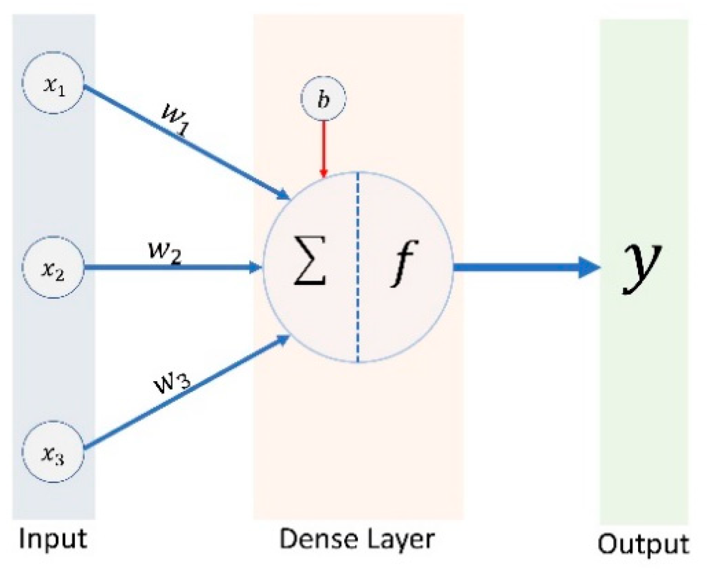
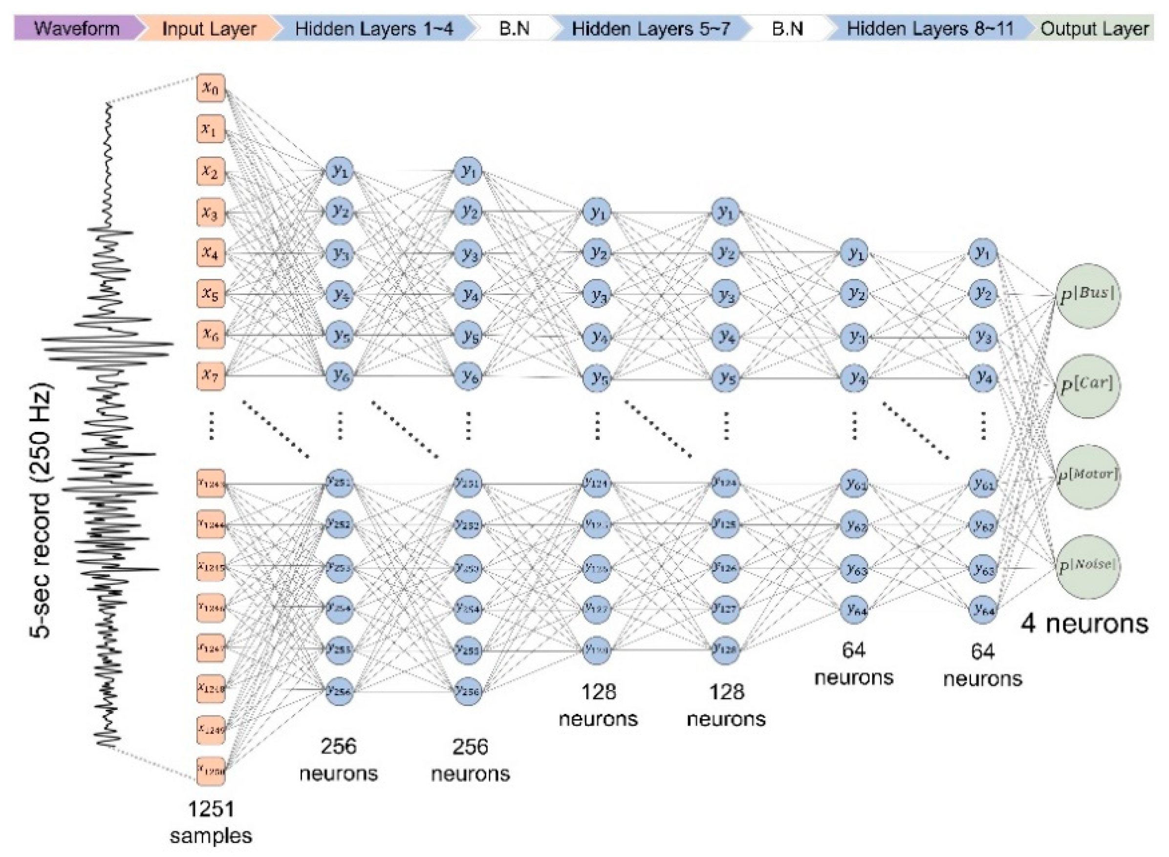
2.1. Deep Neural Network

A deep neural network (DNN) is a simple network with many hidden layers. A large number of hidden layers is advantageous for dealing with time-series data [28]. Our DNN model contains 11 hidden layers. The first four hidden layers each contain 256 neurons, the middle three layers have 128 neurons, and the last four layers have 64 neurons. This decrease in neuron count helps DNN to compress the information into fewer neurons. The last layer, the output layer, contains four neurons representing the four classes in our model (Figure 2). Before each decrease in the size of the hidden layer, we apply batch normalization to avoid internal covariate shifts [35]. The details of the DNN model architecture are given in the Supplementary Material (Table S1).

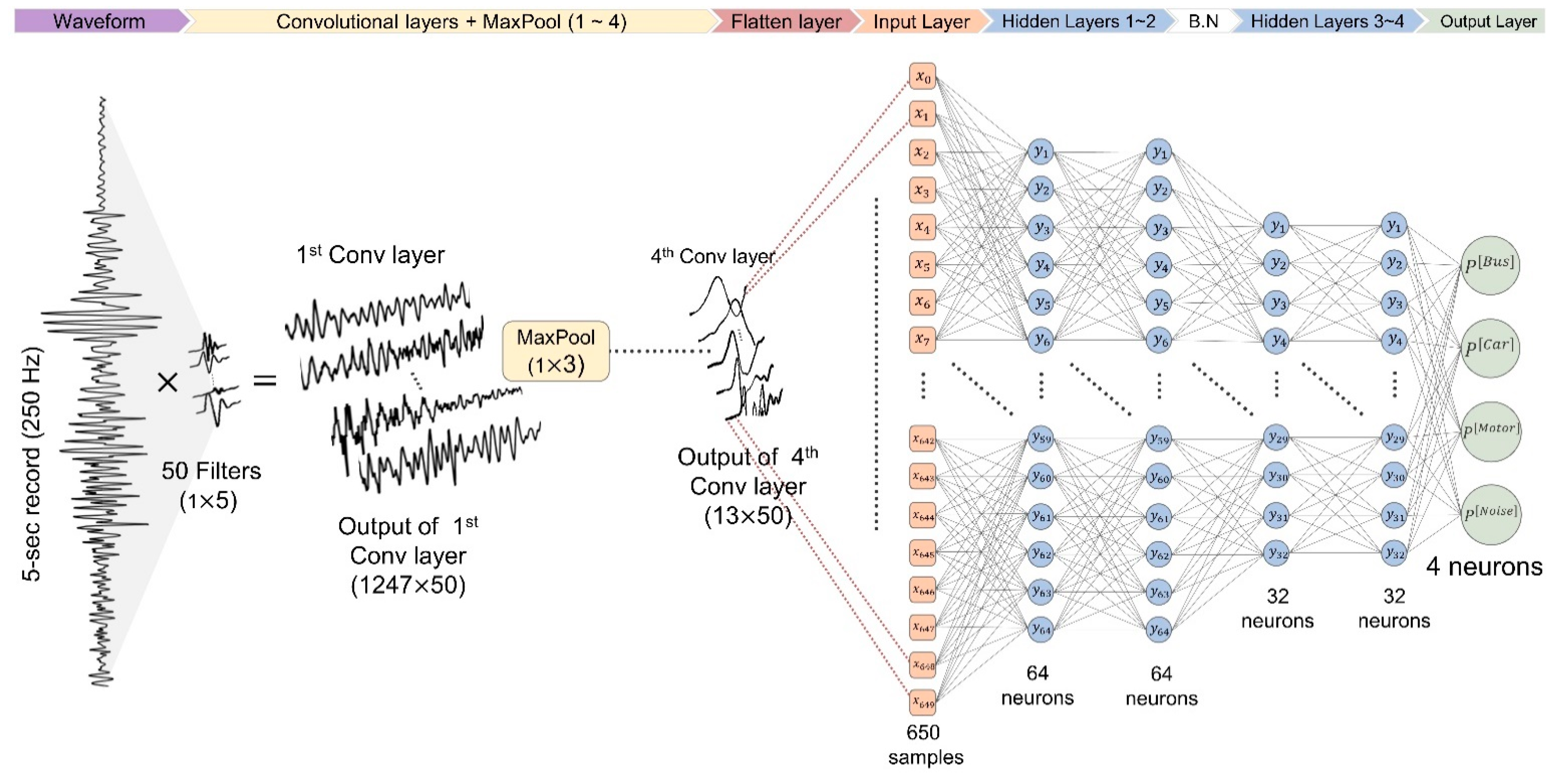
2.2. Convolutional Neural Network

The convolutional neural network (CNN) has become popular for solving problems that contain features such as image recognition and is considered the best algorithm for visual recognition problems [36]. CNN contains a convolutional layer before the main neural network that is made up of multi-channel filters that extract unique features of each class. CNN thus breaks problems into smaller tasks, making the classification task for the next layers much easier [26]. The convolutional layer functions as a feature extractor, and the neural network (also called the fully connected layer) classifies based on features instead of the raw data. The CNN we used for this study contained four convolutional layers with 50 filters (sized 1 × 5) in each layer. We used MaxPool as a downsampling layer with a dimension of (1 × 3) to keep the maximum value of each of the 3 samples. So, the output of the MaxPool layer is one-third of the original data (1247/3 = 415 samples). There are 4 convolutional layers, each followed by a MaxPool layer. The final output of the convolutional layer is 50 channels signal, and each channel contains 13 features. In other words, the output is (13 × 50) the features map. We used a flatten layer to convert this map to a list with 650 variables to introduce it into the fully connected layer.

The fully connected layer contains four hidden layers and a final output layer (Figure 3). The details of the CNN model architecture used in this study are listed in Table S2. We chose four convolutional layers after testing different numbers of layers and considering the trade-offs between accuracy and computational time.

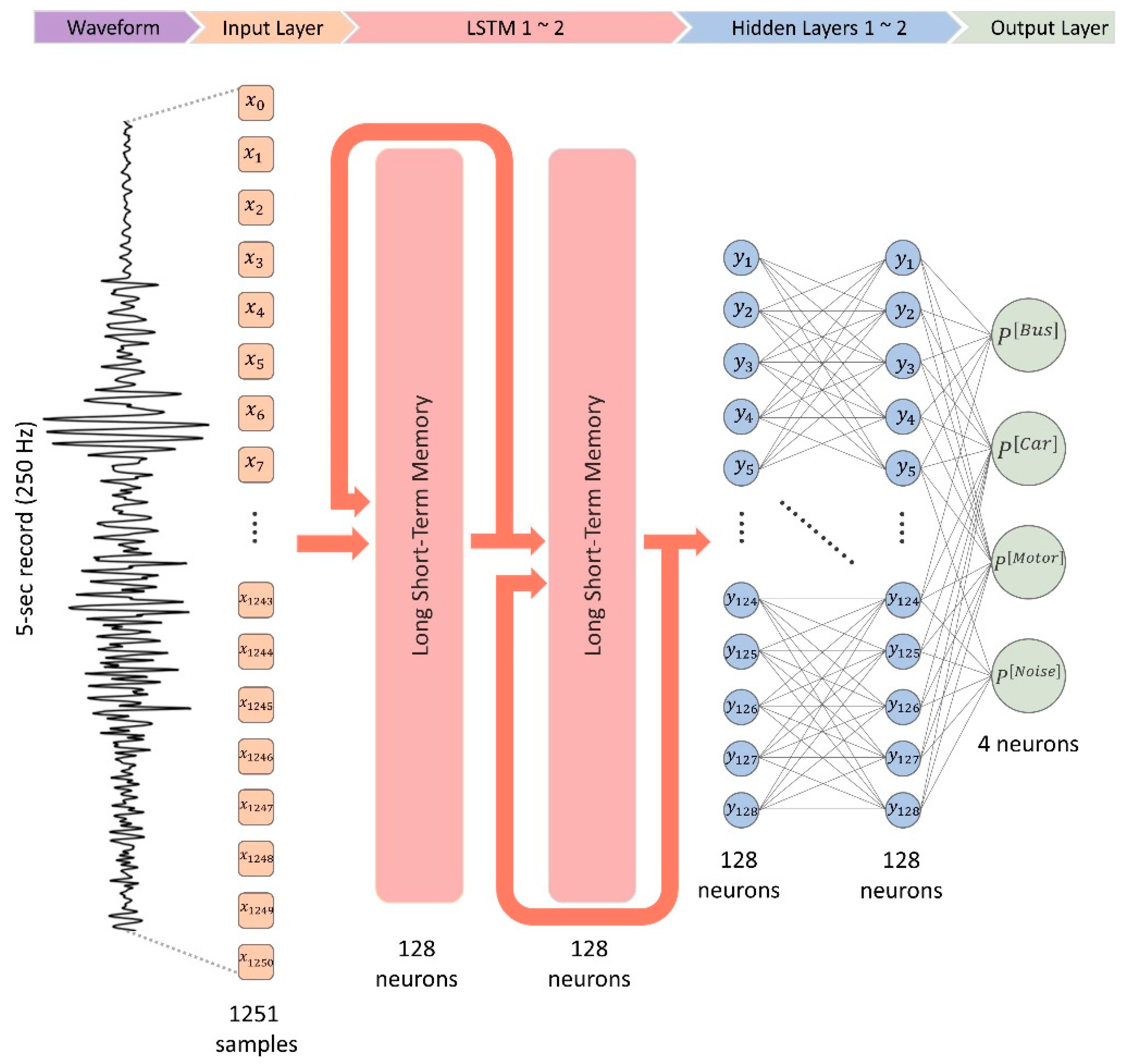
2.3. Recurrent Neural Network

The recurrent neural network (RNN) is a recently developed architecture in which connections between nodes form a directed graph along a temporal sequence, which allows it to exhibit temporal dynamic behavior [3]. RNN is similar to DNN, but it also includes a memory of previous results. Our RNN model used two layers of long short-term memory (LSTM) as shown in Figure 4 and Table S3 in the Supplementary Material. Because LSTM was responsible for the dramatic advancement in speech recognition [37], we anticipated a similar performance gain in seismic recognition.

2.4. Optimization of Weights and Biases

Before using the networks, we optimized the values of weights and biases, using a back-propagation process. Back-propagation occurs during model training, where the data flow from the end of the network to the first layer for another iteration. We repeatedly cycled through a known dataset, calculating the error and optimizing the parameters by minimizing the loss function. To ensure a fair comparison, we adopted cross-entropy for all networks, which expresses the average discrepancy between the predicted class and the true class as follows:

$$\mathrm{E} =-\sum {y^{\prime }}_k \log \left(y_k\right)$$

(4)

where y is the outcome of SoftMax for the k class, and y′k is 1 for a true prediction and 0 for a false one. We used the Adam optimizer [38] for the loss function with a learning rate of 0.001 as well as for monitoring the accuracy and mean square error.

In this study, we used a work frame consisting of the TensorFlow 2.3.0 machine learning platform with graphics processing unit (GPU) support along with the ObsPy, NumPy, and scikit-learn libraries. We used a hardware platform containing dual GeForce RTX 2080 ti GPUs with 64 GB RAM to run all algorithms.

3. Data

3.1. Data Set

In this study, we used geophones to obtain seismic data for different vehicles at Kyushu University in July 2020. We placed the geophones in three stations 15 m apart, located 0.5 m from the road. The vertical motions (vibration) were recorded at a rate of 250 Hz. We tagged vehicles by size as large (e.g., buses and trucks), medium (e.g., private passenger cars), and small (e.g., motorcycles and scooters).

During the experiment, a video camera was used to provide a visual guide for the manual preparation of the training data. Each event (the passage of a vehicle) lasted 2–3 s when the vehicle was close to the geophone. Based on signals at three stations, we estimated the speeds of the vehicles. The speeds of most vehicles used in this experiment were 25~35 km/h, and the maximum speed was 45 km/h. In the training process, we chose clear vehicle signals, eliminating all signals that contained surrounding noise or that overlapped with other vehicles to avoid overfitting the models. The selected events were extracted from the record in the form of windows 5 s long, containing 1251 data points (5 × 250 Hz = 1250 samples). This duration was selected to guarantee the inclusion of the whole seismic waveform. We extracted, on average, 68 waveform windows per geophone station for each of the three-vehicle classes for a total of 612 windows. We also selected 318 waveform windows to represent the noise in our data as the fourth class. These include noise produced by strong winds, bicyclists, walkers, pedestrians pushing a trolley, road maintenance, and ambient noise. These 930 windows constituted the entire input to the three neural networks; examples of each class in the dataset are shown in Figure S1 in the Supplementary Material.

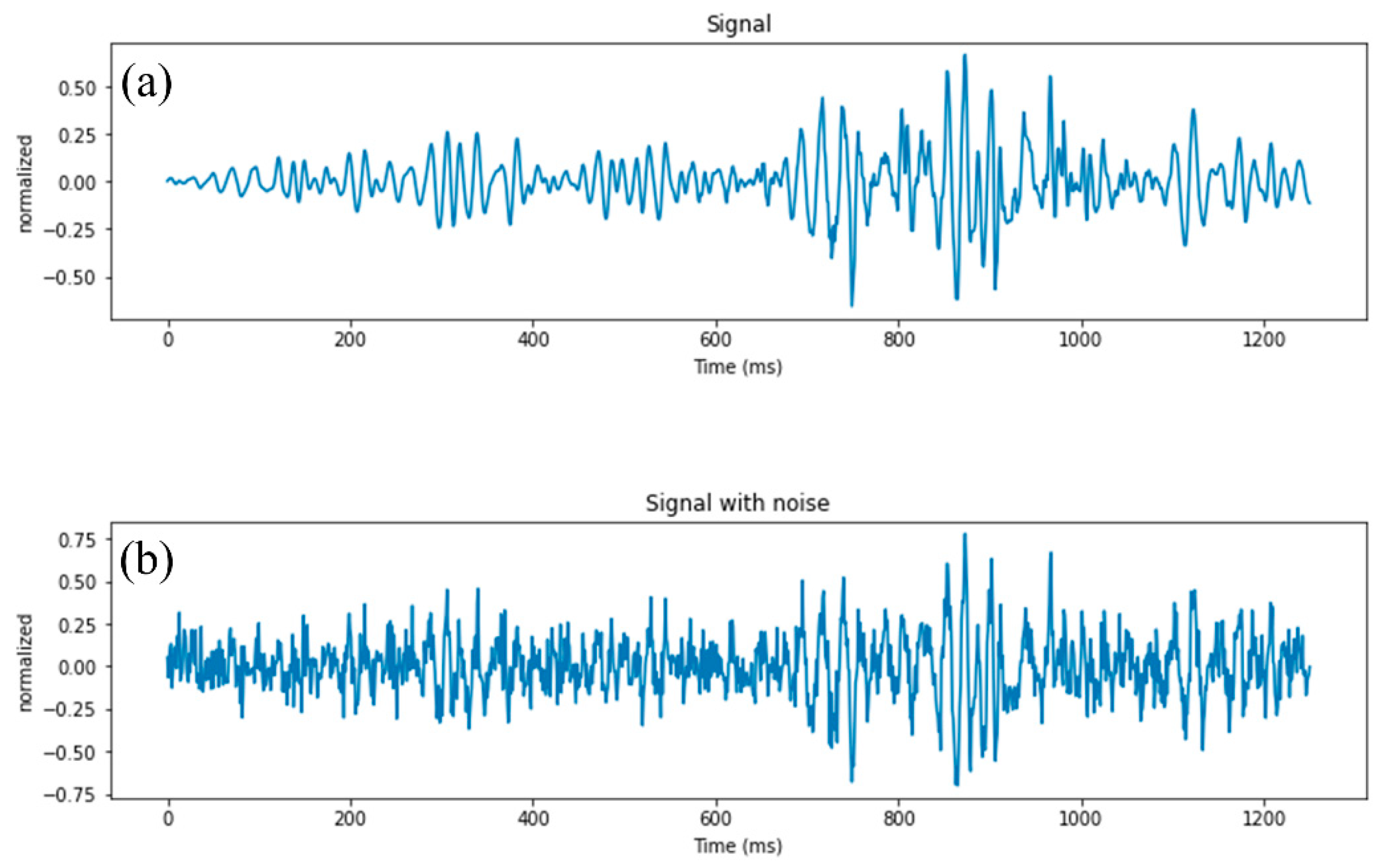
3.2. Training Data Augmentation

Large networks are trained using large amounts of training data to avoid overfitting [36]. Our dataset of 930 samples was inadequate for this purpose; therefore, we generated synthetic data from our initial dataset for training purposes. We added random noise to waveforms to change their signal-to-noise ratio (SNR), as shown in Figure 5. We varied the SNR [39] from 1 to 5 as determined by the following:

$$SNR=\frac{P_{signal}}{P_{noise}}={\left(\frac{A_{signal}}{A_{noise}}\right)}^2,$$

(5)

where P is average power and A is the root mean square amplitude. The resulting augmented dataset used for training contained 4650 synthetic samples (5 × 930).

4. Results

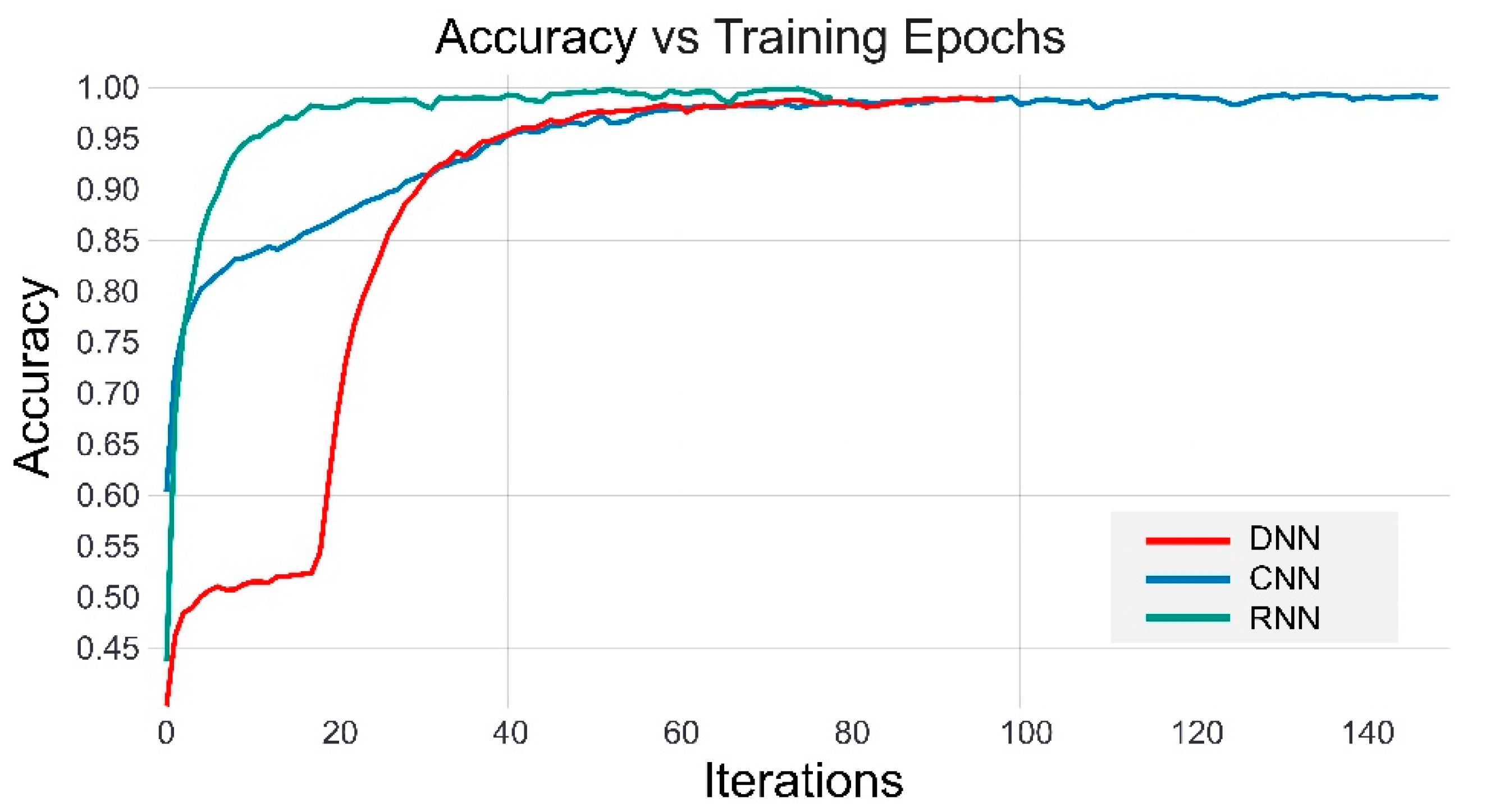
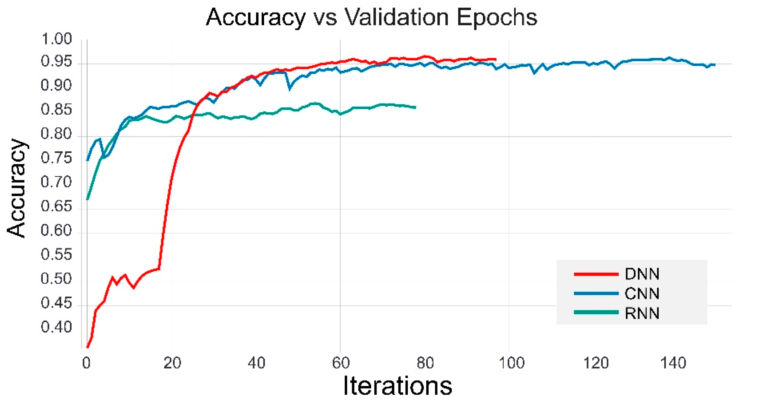
4.1. Training and Validation

We split our augmented dataset randomly into three portions, using the scikit-learn splitting function, dedicating 60% for training, 20% for validation, and 20% for testing. We used the same training set for each of the three networks and trained them over 150 iterations, then selected the model with the best validation accuracy. We also improved our training experience and prevented overfitting in two ways.

First, we applied early stopping in which the networks monitored the validation accuracy and terminated the training when accuracy did not increase for 20 iterations. Second, we set a 30% dropout chance for all weights and biases. So, in each iteration, all weights and biases have a 30% chance to be ignored in the training process. The dropout technique improves the independence of the individual weights [40]. Training took a short computation time: DNN took 87 s, CNN took 112 s, and RNN took 56 s. Because of early stopping, DNN and RNN trained for less than 150 iterations. All models showed a great improvement during training, reaching accuracies close to 99% (Figure 6).

In the validation process, we checked the models’ performance with new data or data that were not used in the training process. The models did not display any overfitting, thanks to the early stopping that curtailed training before any degradation of the validation accuracy. The resulting validation curve represents the generality of the model. Both DNN and CNN reached accuracies of approximately 97%, whereas RNN validation accuracy was approximately 85% (Figure 7).

We also monitored the improvements in loss function and mean square error (Figure S2 in the Supplementary Material).

Table 2. Performances of networks for training (3420 waveforms) and validation (1140 waveforms).

	DNN	CNN	RNN
Time (s): Total training (Average per epoch 1)	87 (0.89)	112 (0.74)	56 (0.69)
Accuracy (%): Training (Validation)	98.6 (95.6)	99.1 (94.7)	99.2 (86.1)
Loss: Training (Validation)	7.80 × 10−2 (0.293)	2.77 × 10−2 (0.240)	3.52 × 10−2 (1.070)
Mean square error: Training (Validation)	6.02 × 10−3 (0.019)	3.58 × 10−3 (0.023)	2.98 × 10−3 (0.065)

¹ Each epoch includes 4560 waveforms of 5 s each.

summarizes the performance of the three models during training and validation.

4.2. Classification Accuracy

We tested the classification accuracy of the three networks using 20% of the dataset (1116 samples). We compared the results with those of a similarity method for seismic event detections called template matching [41]. We randomly selected 50 waveforms for each vehicle class from the training data to be used as templates. We also recorded 15 min of new data for this experiment. We took into consideration factors that might affect the data, including the time of recording, location of stations, and types of geophones. The networks were not retrained before this exercise, and the templates also were not changed.

The resulting detection accuracies are listed in

Table 3. Performances and running time (1140 waveforms) of networks and template matching.

	Template Matching	DNN	CNN	RNN
Time (ms)	560	74	67	55
Accuracy (%)	77.3	97.8	96.6	85.3
Mean square error	N/A	0.009	0.014	0.063

. DNN achieved the best accuracy, with 97.8% correct detections, followed by CNN with 96.6% and RNN with 85.3%. Template matching had much lower classification accuracy and took an order of magnitude longer to process the testing data.

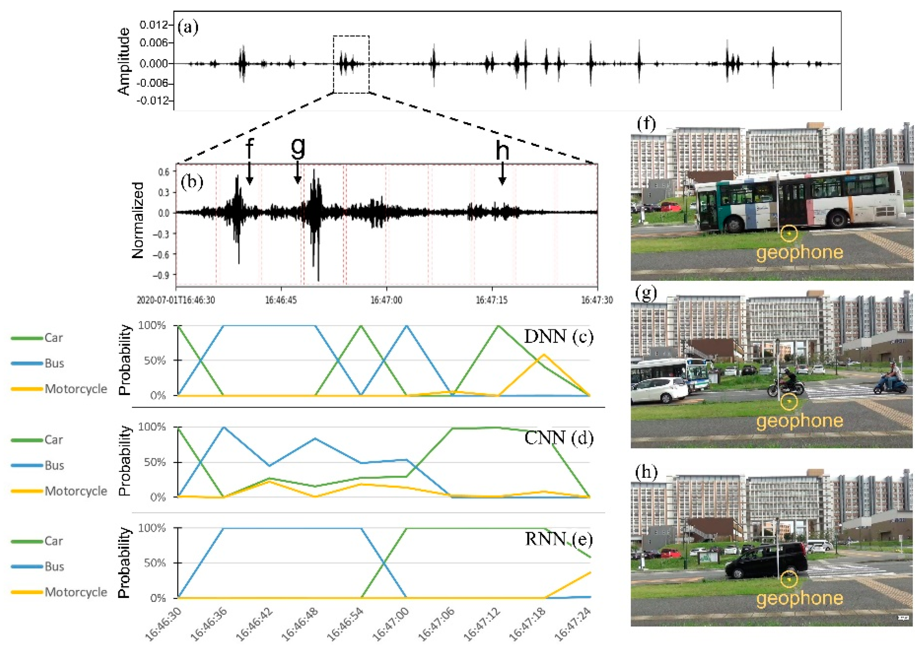
4.3. Vehicle Detection in Continuous Records

Because practical applications involve records longer than 5 s, we tested the framework for detecting vehicles using the 15 min continuous waveform dataset described in the previous section. The single-channel waveforms were cut into windows 5 s long, with a gap between consecutive windows of 1 s to reduce the potential for redundant detections (Figure 8).

Thanks to the feature extraction implemented in the convolutional layer, CNN was able to detect vehicles of different classes with overlapping seismic records. In the example of Figure 9, a truck, a lightweight car, and a motorcycle passed the geophone in quick succession.

We used a 90% probability threshold to determine the predicted vehicle class. The 15 min record included 93 different vehicles.

Table 4. Precision and recall of networks on a 15 min data record, including 16 large, 49 medium, and 28 small Vehicles.

	Clas	DNN	CNN	RNN
Precision (%)	Big (bus, trucks)	100	100	88.8
	Medium (light car)	75.8	97.9	81.3
	Small (motorcycle)	90.4	90.9	80
Recall (%)	Big (bus, trucks)	93.8	100	100
	Medium (light car)	95.9	95.2	97.9
	Small (motorcycle)	67.8	72.2	85.7
Average Precision (Recall) (%)		88.7 (85.8)	96.2 (89.1)	83.3 (94.5)

shows the performance of the three models in terms of precision and recall per vehicle class. Precision represents the percentage of correct declarations among all declarations made by the model, and recall represents the percentage of correct declarations among all declarations:

$${\mathrm{Precision}}_{Class}=\frac{ T{P}_{Class}}{T{P}_{Class}+F{P}_{Class}}$$

(6)

$${\mathrm{Recall}}_{Class}=\frac{ T{P}_{Class}}{T{P}_{Class}+F{N}_{Class}}$$

(7)

where TP stands for true positive, FP stands for false positive, and FN stands for false-negative [42]. We used visual data, as shown in Figure 8f–h and Figure 9a to determine the true positive/true negative and ensure calculating the real accuracy for our method. By clear margins, CNN had the best precision and RNN had the best recall.

4.4. Scalability to Long Records

One desirable feature of a seismic-based system for traffic monitoring is its ability to operate continuously with minimal supervision, which means the system needs to deal with long records (e.g., several weeks or months). For that reason, we evaluated the computational cost of the three models, ignoring their accuracy and focusing on the scalability of networks to handle large records. We chose 1 h of data to measure running time and memory usage, then repeated the measurements after successively doubling the size of the dataset to a maximum of 1024 h (nearly 43 days) (Figure 10). CNN interpreted a month-long (720 h) record in 70 min, a computation time 10% faster than DNN. CNN also had the lowest memory usage, requiring 40% less memory than RNN. In terms of computational cost for long records, CNN was more efficient than DNN and RNN.

5. Discussion

This study achieved good performance in probabilistic vehicle detection, and it confirmed the effectiveness of long-term monitoring. The neural networks outperformed template matching in computational cost and in terms of accuracy and generalization. CNN, in particular, achieved state-of-the-art performance in analyzing new data.

CNN was able to detect and identify these vehicles by their frequency components, even when their signals overlapped. For example, at the time of 16:33:43 in Figure 9, CNN determined a 40% probability for a truck and a 60% probability for a car, even though the truck’s signal was stronger than that of the car. We attribute this ability to the convolutional filters in CNN which, unlike RNN and DNN, input extracted features to the dense layers. Although RNN had the highest recall, CNN had the highest precision. Because CNN detected the overlapped vehicles with a probability of less than 90% (Figure 8d and Figure 9), these identifications were not counted as detections, but the recall score could be enhanced by decreasing the threshold probability to below 90%. However, CNN and other networks have failed to recognize the existence of overlapped vehicles within the same type. The current network’s architectures were not designed to count multiple vehicles. This problem could be overcome by using more than one receiver.

The relatively poor performance of RNN may stem from the intrinsic conflict between the independence of vehicle events and the inclusion of the LSTM layer in RNN that detects sequences of events. The RNN tries to create a long memory for the sequence of vehicle classes, but the succession of vehicle events is essentially random.

All networks were similar in their computational cost. However, CNN had the shortest running time for very long records. On average, CNN needed 5 min to interpret a 1-day record and 70 min to interpret a 1-month record. DNN had the lowest memory demand of the three models, using a maximum of 1.72 GB of the system RAM; however, memory usage was tolerable for the other two models (Figure 10). Theoretically, the cost of memory usage is constant at all levels of traffic because the neural network only needs to store the weights and biases [29]. Ultimately, the proposed system based on seismic signals has been proved as an alternative solution for vehicle classification with an accuracy of up to 97%, close to the previously adopted systems based on the automatic visual classification (90~99%) and the loop detector systems (99% accuracy). The systems we tested did not have high power requirements or high computational costs and were physically unobtrusive. More importantly, the traffic monitoring system based on seismic data was able to detect and classify vehicles reliably without violating the public’s privacy.

6. Conclusions

Machine learning proved to be an effective and low-cost technique to enable traffic monitoring in real-time based on seismic data. In this study, we evaluated three neural network systems for this purpose and demonstrated that CNN provided the best performance in terms of accuracy and speed. CNN also surpassed the others in its ability to detect overlapping signals. RNN did not perform as well as the others for traffic monitoring because its intrinsic reliance on temporal sequences conflicts with the random nature of traffic data. Although seismic data can be used for traffic monitoring, all neural networks have a shortcoming in terms of counting vehicles because they cannot identify the presence of multiple vehicles of the same class within a waveform frame.

The main limitation of neural networks is the human effort expended in acquiring and compiling a suitable amount of training data. We augmented our dataset by adding random noise. Although the models can be deployed without extra training, we recommend retraining the model as much as possible to guarantee the best performance in the generalization.

Neural networks that process seismic data offer compelling advantages over current approaches to traffic monitoring. The seismic record has small file sizes compared to videos and other types of monitoring data. Because the system is simple and passive, consisting of a few geophones, it can be implemented for months at a time without supervision. The recorded data can be analyzed at a low computational cost to give clear statistical information for vehicles during the implementation period. This makes the proposed system suitable for use in hard-to-access roads. Our favored method, based on CNN, is suitable for continuous records of a month or longer; CNN was able to process a month’s worth of data in approximately an hour.

The proposed method can be extended by investigating the feasibility of using it to estimate more types of traffic data, such as speed, direction, and if the driving follows a probable manner or not (i.e., drive while drunk). Since we identified the car type via our CNN-based approach, the estimation of the speed of the vehicles could be possible; we presently are investigating accurate speed estimation systems. It may also be possible to extend a similar approach to other types of transportation, such as vessels, bicycles, foot traffic, or airplanes.

References

1. Lee, H.; Coifman, B. Using LIDAR to Validate the Performance of Vehicle Classification Stations. J. Intell. Transp. Syst. Technol. Plan. Oper. 2015, 19, 355–369. [Google Scholar] [CrossRef]
2. U.S. Federal Highway Administration (Ed.) Traffic Monitoring Guide—Updated October 2016; Office of Highway Policy Information: Washington, DC, USA, 2016. [Google Scholar]
3. Abiodun, O.I.; Jantan, A.; Omolara, A.E.; Dada, K.V.; Mohamed, N.A.E.; Arshad, H. State-of-the-art in artificial neural network applications: A survey. Heliyon 2018, 4, e00938. [Google Scholar] [CrossRef] [PubMed] [Green Version]
4. Won, M. Intelligent Traffic Monitoring Systems for Vehicle Classification: A Survey. IEEE Access 2019, 8, 73340–73358. [Google Scholar] [CrossRef]
5. Coifman, B.; Neelisetty, S. Improved speed estimation from single-loop detectors with high truck flow. J. Intell. Transp. Syst. Technol. Plan. Oper. 2014, 18, 138–148. [Google Scholar] [CrossRef]
6. Jeng, S.T.; Chu, L. A high-definition traffic performance monitoring system with the Inductive Loop Detector signature technology. In Proceedings of the 2014 17th IEEE International Conference on Intelligent Transportation Systems, ITSC 2014, Qingdao, China, 8–11 October 2014; Institute of Electrical and Electronics Engineers Inc.: Piscataway Township, NJ, USA, 2014; pp. 1820–1825. [Google Scholar]
7. Wu, L.; Coifman, B. Improved vehicle classification from dual-loop detectors in congested traffic. Transp. Res. Part C Emerg. Technol. 2014, 46, 222–234. [Google Scholar] [CrossRef]
8. Wu, L.; Coifman, B. Vehicle length measurement and length-based vehicle classification in congested freeway traffic. Transp. Res. Rec. 2014, 2443, 1–11. [Google Scholar] [CrossRef]
9. Balid, W.; Refai, H.H. Real-time magnetic length-based vehicle classification: Case study for inductive loops andwireless magnetometer sensors in Oklahoma state. Transp. Res. Rec. 2018, 2672, 102–111. [Google Scholar] [CrossRef]
10. Li, Y.; Tok, A.Y.C.; Ritchie, S.G. Individual Truck Speed Estimation from Advanced Single Inductive Loops. Transp. Res. Rec. 2019, 2673, 272–284. [Google Scholar] [CrossRef]
11. Lamas-Seco, J.J.; Castro, P.M.; Dapena, A.; Vazquez-Araujo, F.J. Vehicle classification using the discrete fourier transform with traffic inductive sensors. Sensors 2015, 15, 27201–27214. [Google Scholar] [CrossRef] [PubMed] [Green Version]
12. Odat, E.; Shamma, J.S.; Claudel, C. Vehicle Classification and Speed Estimation Using Combined Passive Infrared/Ultrasonic Sensors. IEEE Trans. Intell. Transp. Syst. 2018, 19, 1593–1606. [Google Scholar] [CrossRef]
13. Dong, H.; Wang, X.; Zhang, C.; He, R.; Jia, L.; Qin, Y. Improved Robust Vehicle Detection and Identification Based on Single Magnetic Sensor. IEEE Access 2018, 6, 5247–5255. [Google Scholar] [CrossRef]
14. Belenguer, F.M.; Martinez-Millana, A.; Salcedo, A.M.; Nunez, J.H.A. Vehicle Identification by Means of Radio-Frequency-Identification Cards and Magnetic Loops. IEEE Trans. Intell. Transp. Syst. 2019, 21, 5051–5059. [Google Scholar] [CrossRef]
15. Li, F.; Lv, Z. Reliable vehicle type recognition based on information fusion in multiple sensor networks. Comput. Netw. 2017, 117, 76–84. [Google Scholar] [CrossRef]
16. Carli, R.; Dotoli, M.; Epicoco, N.; Angelico, B.; Vinciullo, A. Automated evaluation of urban traffic congestion using bus as a probe. In Proceedings of the 2015 IEEE International Conference on Automation Science and Engineering (CASE), Gothenburg, Sweden, 24–28 August 2015; pp. 967–972. [Google Scholar]
17. Ahmed, S.H.; Bouk, S.H.; Yaqub, M.A.; Kim, D.; Song, H.; Lloret, J. CODIE: Controlled Data and Interest Evaluation in Vehicular Named Data Networks. IEEE Trans. Veh. Technol. 2016, 65, 3954–3963. [Google Scholar] [CrossRef]
18. Carli, R.; Dotoli, M.; Epicoco, N. Monitoring traffic congestion in urban areas through probe vehicles: A case study analysis. Internet Technol. Lett. 2018, 1, e5. [Google Scholar] [CrossRef] [Green Version]
19. Wang, S.; Zhang, X.; Cao, J.; He, L.; Stenneth, L.; Yu, P.S.; Li, Z.; Huang, Z. Computing urban traffic congestions by incorporating sparse GPS probe data and social media data. ACM Trans. Inf. Syst. 2017, 35, 1–30. [Google Scholar] [CrossRef]
20. Litman, T. Developing indicators for comprehensive and sustainable transport planning. Transp. Res. Rec. 2007, 2007, 10–15. [Google Scholar] [CrossRef] [Green Version]
21. Martin, P.T.; Feng, Y.; Wang, X. Detector Technology Evaluation; Mountain-Plains Consortium: Fargo, ND, USA, 2003. [Google Scholar]
22. William, P.E.; Hoffman, M.W. Classification of military ground vehicles using time domain harmonics’amplitudes. IEEE Trans. Instrum. Meas. 2011, 60, 3720–3731. [Google Scholar] [CrossRef] [Green Version]
23. Ketcham, S.A.; Moran, M.L.; Lacombe, J.; Greenfield, R.J.; Anderson, T.S. Seismic source model for moving vehicles. IEEE Trans. Geosci. Remote Sens. 2005, 43, 248–256. [Google Scholar] [CrossRef]
24. Moran, M.L.; Greenfield, R.J. Estimation of the acoustic-to-seismic coupling ratio using a moving vehicle source. IEEE Trans. Geosci. Remote Sens. 2008, 46, 2038–2043. [Google Scholar] [CrossRef]
25. Jin, G.; Ye, B.; Wu, Y.; Qu, F. Vehicle Classification Based on Seismic Signatures Using Convolutional Neural Network. IEEE Geosci. Remote Sens. Lett. 2019, 16, 628–632. [Google Scholar] [CrossRef]
26. Zhao, T. Seismic facies classification using different deep convolutional neural networks. In Proceedings of the 2018 SEG International Exposition and Annual Meeting, SEG 2018, Anaheim, CA, USA, 14–19 October 2018; pp. 2046–2050. [Google Scholar]
27. Shimshoni, Y.; Intrator, N. Classification of seismic signals by integrating ensembles of neural networks. IEEE Trans. Signal Process. 1998, 46, 1194–1201. [Google Scholar] [CrossRef] [Green Version]
28. Titos, M.; Bueno, A.; Garcia, L.; Benitez, C. A Deep Neural Networks Approach to Automatic Recognition Systems for Volcano-Seismic Events. IEEE J. Sel. Top. Appl. Earth Obs. Remote Sens. 2018, 11, 1533–1544. [Google Scholar] [CrossRef]
29. Perol, T.; Gharbi, M.; Denolle, M. Convolutional neural network for earthquake detection and location. Sci. Adv. 2018, 4, e1700578. [Google Scholar] [CrossRef] [PubMed] [Green Version]
30. Yuan, S.; Liu, J.; Wang, S.; Wang, T.; Shi, P. Seismic Waveform Classification and First-Break Picking Using Convolution Neural Networks. IEEE Geosci. Remote Sens. Lett. 2018, 15, 272–276. [Google Scholar] [CrossRef] [Green Version]
31. Evans, N. Automated Vehicle Detection and Classification Using Acoustic and Seismic Signals. Ph.D. Thesis, University of York, York, UK, 2010. [Google Scholar]
32. Grossberg, S.; Rudd, M.E. A neural architecture for visual motion perception: Group and element apparent motion. Neural Netw. 1989, 2, 421–450. [Google Scholar] [CrossRef]
33. Nair, V.; Hinton, G.E. Rectified linear units improve Restricted Boltzmann machines. In Proceedings of the ICML 2010—27th International Conference on Machine Learning, Haifa, Israel, 21–24 June 2010; pp. 807–814. [Google Scholar]
34. Shim, K.; Lee, M.; Choi, I.; Boo, Y.; Sung, W. SVD-Softmax: Fast Softmax Approximation on Large Vocabulary Neural Networks. In Proceedings of the Advances in Neural Information Processing Systems, Long Beach, CA, USA, 4–9 December 2017; Volume 30, pp. 5463–5473. [Google Scholar]
35. Ioffe, S.; Szegedy, C. Batch Normalization: Accelerating Deep Network Training by Reducing Internal Covariate Shift. In Proceedings of the 32nd International Conference on Machine Learning (ICML 2015), Lille, France, 6–11 July 2015; Volume 1, pp. 448–456. [Google Scholar]
36. Waldeland, A.U.; Jensen, A.C.; Gelius, L.-J.; Solberg, A.H.S. Convolutional neural networks for automated seismic interpretation. Lead. Edge 2018, 37, 529–537. [Google Scholar] [CrossRef]
37. Hochreiter, S.; Schmidhuber, J. Long Short-Term Memory. Neural Comput. 1997, 9, 1735–1780. [Google Scholar] [CrossRef]
38. Kingma, D.P.; Ba, J.L. Adam: A method for stochastic optimization. In Proceedings of the 3rd International Conference on Learning Representations, ICLR 2015, San Diego, CA, USA, 7–9 May 2015. [Google Scholar]
39. Tyagi, V.; Kalyanaraman, S.; Krishnapuram, R. Vehicular Traffic Density State Estimation Based on Cumulative Road Acoustics. IEEE Trans. Intell. Transp. Syst. 2012, 13, 1156–1166. [Google Scholar] [CrossRef]
40. Srivastava, N.; Hinton, G.; Krizhevsky, A.; Sutskever, I.; Salakhutdinov, R. Dropout: A Simple Way to Prevent Neural Networks from Overfitting. J. Mach. Learn. Res. 2014, 15, 1929–1958. [Google Scholar]
41. Skoumal, R.J.; Brudzinski, M.R.; Currie, B.S.; Levy, J. Optimizing multi-station earthquake template matching through re-examination of the Youngstown, Ohio, sequence. Earth Planet. Sci. Lett. 2014, 405, 274–280. [Google Scholar] [CrossRef] [Green Version]
42. Davis, J.; Goadrich, M. The relationship between precision-recall and ROC curves. In Proceedings of the 23rd ACM International Conference Proceeding Series, Pittsburgh, PA, USA, 25–29 June 2006; Volume 148, pp. 233–240. [Google Scholar]
Figure 1. A simple neural network illustrating Equation (1). Inputs (x) multiplied by weights (w) are summed in the dense layer, adding bias (b), then the activation function (f) is applied to get the output.
Applsci 11 04590 g001
Figure 2. The DNN architecture used in this study. The 5 s waveform is discretized as 1251 samples and fed to 11 dense layers, including two batch normalization (B.N) operations between hidden layers 4 and 5 and hidden layers 7 and 8. The model produces four values indicating the probability of each vehicle class.
Applsci 11 04590 g002
Figure 3. The CNN architecture used in this study. Five convolutional layers each contain 50 filters and a MaxPool layer to downsample the amount of contained data. The convolutional and flattening layers condense the original 1251 samples to 650 samples containing filtered features. These are introduced to a neural network with four hidden layers and one batch normalization (B.N) operation. The model produces four values, indicating the probability of each vehicle class.
Applsci 11 04590 g003
Figure 4. The RNN architecture used in this study. The model contains two LSTM layers and two hidden layers. The model produces four values, indicating the probability of each vehicle class.
Applsci 11 04590 g004
Figure 5. (a) Seismic signal of a bus before adding noise. (b) Seismic signal after adding noise to produce a signal to noise ratio of 6.
Applsci 11 04590 g005
Figure 6. Plot showing the improvement in accuracy with increasing iterations during the training process for DNN (red), CNN (blue), and RNN (green). RNN was stopped early at 79 iterations and DNN was stopped at 97 iterations.
Applsci 11 04590 g006
Figure 7. Plot showing the improvement in accuracy during the validation process for DNN (red), CNN (blue), and RNN (green).
Applsci 11 04590 g007
Figure 8. (a) A continuous seismic record 20 min long. (b) Detail of (a) showing a data window 1 min long divided into 5 s waveforms (red boxes) with gaps of 1 s between them. (c) The probability of vehicle types during the window in (c) is estimated using DNN, (d) CNN, and (e) RNN. Events during the window include the passage of (f) a bus, (g) a motorcycle, and (h) a car in mixed traffic. The vibrations recorded at times of pictures (f), (g,h) are displayed on panel (b).
Applsci 11 04590 g008
Figure 9. (a) A video frame documenting several vehicles passing the receiver at time 16:33:43. (b) The seismic noise generated a 10 s window. (c) Vehicle type probabilities estimated by CNN at intervals of 1 s during the window in (b) contain 10 interpretation points with 80% overlapping.
Applsci 11 04590 g009
Figure 10. (a) The run time required by DNN (red), CNN (blue), and RNN (green) to process a seismic record 1024 h long (2.35 GB). (b) The memory usage required by the three networks to process the long seismic record, including the RAM usage and TensorFlow in the backend.
Applsci 11 04590 g010