Article

Convergency and Stability of Explicit and Implicit Schemes in the Simulation of the Heat Equation

by
Franyelit Suárez-Carreño
1,* and
Luis Rosales-Romero
2
1
Industrial Engineering Career, Faculty of Engineering and Applied Sciences, University of the Americas, Quito 170902, Ecuador
2
Basic Science Department, Physics Section, Polytechnic University of Venezuela, UNEXPO, Puerto Ordaz 8050, Venezuela
*
Author to whom correspondence should be addressed.
Appl. Sci. 2021, 11(10), 4468; https://doi.org/10.3390/app11104468
Submission received: 10 April 2021 / Revised: 27 April 2021 / Accepted: 27 April 2021 / Published: 14 May 2021
(This article belongs to the Topic Metallurgical and Materials Engineering)

Abstract

:

Featured Application

The authors show some computational highlights in the application of the system described above.

Abstract

Some strategies for solving differential equations based on the finite difference method are presented: forward time centered space (FTSC), backward time centered space (BTSC), and the Crank-Nicolson scheme (CN). These are developed and applied to a simple problem involving the one-dimensional (1D) (one spatial and one temporal dimension) heat equation in a thin bar. The numerical implementation in this work can be used as a preamble to introduce a method of solving the heat equation that can be implemented in problems in the area of finances. The results of implementing the software on very fine meshes (unidimensional), and with relatively small-time steps, are shown. Through mesh refinement, it was possible to obtain a better temperature distribution in the thin bar between a range of points. The heat equation was solved numerically by testing both implicit (CN) and explicit (FTSC and BTSC) methods. The examples show that the implemented schemes conform to theoretical predictions and that truncation errors depend on mesh, spacing, and time step.

1. Introduction

Most physical phenomena are represented by partial differential equations. Steady-state physical problems or time evolution problems are modeled through elliptic and parabolic partial differential equations, respectively; these equations are difficult to solve by analytical methods when the initial and boundary conditions are not simple. An example of this is shown in [1,2,3] and references therein, where several equations of physics-mathematics describing phenomena related to continuous element dynamics, electrodynamics, quantum mechanics, and mass and heat transfer phenomena are highlighted. For the solution of some of these equations, they use methods such as the Fourier Method, the Riemann Integration, and the use of the Green’s Function [4,5,6,7,8]. However, these procedures do not always guarantee analytical solutions that illustrate the behavior of a mechanical system; this is where numerical methods provide powerful techniques that allow a solution as close as possible to the reality of a specific problem.
The numerical methods developed by Harriot [9,10,11,12,13,14,15] were used to solve equations and transcended in an important way to engineering in 1943 when Courant developed the finite element method. Courant used the numerical methods of variation proposed by Ritz to obtain approximate solutions for mechanical systems [16,17]. The Courant–Friedrichs–Lewy (CFL) condition is a necessary condition for convergence in the numerical solution of partial differential equations with partial differentials. A case of special importance is when time discretization schemes are used as a numerical solution. As a consequence, in many simulations, the time step has to be less than a characteristic value; otherwise, the code may be unstable and not yield the correct results.
Thus, simulations are an effective tool in applied sciences to find solutions and predict their behavior. Additionally, they allow the mathematical recreation of physical processes that frequently appear in engineering [18,19,20]. The use of simulations to study partial differential equations, in particular the diffusion equation, normally requires a careful study of numerical methods, the algorithms to be used, and the fundamental processes to be included in the simulation. A simulation differs from a mathematical model in that the former is a representation at each instant of the process to be simulated, while the model is a mathematical abstraction of the fundamental equations necessary to analyze that phenomenon. Normally, the use of a simulation to study a given problem requires careful planning of the mathematical model (partial differential equations and initial and boundary conditions) to be used and of the algorithms necessary to solve the model. Numerical methods are used to determine the numerical solution of problems for which the analytical solution may or may not be known. These allow the translation of complicated mathematical schemes using algorithms, the results of which can be contrasted with the analytical solutions, in cases where such solutions exist.
In this work, the heat conduction equation is simulated to obtain the temperature patterns in a thin bar [21,22,23]. The analysis of non-stationary heat transfer is of practical interest, not only because of the importance that cooling and heating processes have in a large number of industrial applications but also because of their similarity with several other equations of physics-mathematics that present the same difficulties to be solved numerically. Among the problems directly related to non-stationary heat transfer problems are the starting and stopping of machines, processes that can lead, on the one hand, to the appearance of important thermal loads on the solid with the consequent deterioration (turbine blades, for example), and on the other hand, to an increased emission of polluting species (steam generators, gas turbines, and alternative internal combustion engines, among others).
For the reasons mentioned above, the efficient and accurate solution of the time-dependent differential equations of heat transfer plays a fundamental role, not only because of the number of engineering problems they represent but also as an initial or test case for many other more complex problems, in particular, the equations of fluid mechanics, whose correct solution depends on the efficiency shown by the different methods in the solution of the heat transfer equations [1,2,3].
The increasing use of multiprocessor-based computers, either using parallel programming or multiple processors, has recently encouraged the use of explicit methods, which are much more apt to be parallelized due to their local information processing condition [4,5]. It could be said that an explicit method, although more computationally expensive than an implicit method, is much more likely to be more efficient in parallel computation, and may even exceed it, depending on the number of parallel processors used [6,7,8].
In this work, we try to verify the results obtained previously, using implicit and explicit methods that are stable for time steps much larger than those normally used in this type of simulation with time dependence. The time steps achieved are, for similar accuracy, of the same order as those used in the implicit methods. In this way, all the advantages concerning the ease of parallel processing typical of the explicit ones are maintained with the advantages of the implicit ones concerning their stability for large time steps [24,25].
N-soliton solutions could also be generated for (1 + 1)-dimensional integrable differential equations; however, it is not of interest for this study to treat heat waves as solitons. The interest of this research is to test different discretization schemes in the solution of partial differential equations; to study the stability and convergence of each discretization scheme in the one-dimensional heat diffusion equation; and, finally, to conclude which scheme is more advantageous for future applications in various areas of interest.

2. The Heat Equation

In engineering problems, it is common to find mathematical models that include partial differential equations [26,27,28,29]. The analytical solution provides a better understanding of the behavior of some phenomena since it can be determined at any instant of time. In general, it is not possible to determine this solution due to the non-linearity of the equations that constitute the mathematical model or due to the domain where the model is studied. Numerical methods in science and engineering provide a tool that allows translating mathematical models into computational procedures, whose results can be contrasted with the analytical solutions, in those cases where they exist. In the following, an algorithm for solving partial differential equations is shown, using the one-dimensional diffusion equation as a model problem. The choice of the same one is made based on its multiple applications in problems of mechanics using the finite difference method to determine the numerical solution of the diffusion equation using an explicit method and the implicit CN method [30,31].
The one-dimensional 1D heat equation is expressed by Equation (1)
t = α 2 x 2                           0 x L ,             t 0
where = x , t is the temperature and α is a constant coefficient. Equation (1) is a model of transient heat conduction in a metallic segment of length L (physical domain). The material property α is the thermal diffusivity. In a practical calculation, the solution is obtained only for a finite time, tmax.
The solution to Equation (1) requires the specification of boundary conditions at x = 0 and x = L, and initial conditions at t = 0. The initial and boundary conditions are [32,33]:
ϕ 0 , t = ϕ 0 ,   ϕ L , t = ϕ L   ϕ x , 0 = ƒ 0 x
Other boundary conditions exist, represented by the gradient of the function at the ends of the thin bar [34,35], or mixed conditions are also considered in the simulations. To keep the presentation as simple as possible, only the conditions in Equation (2) are considered in this article (Figure 1).

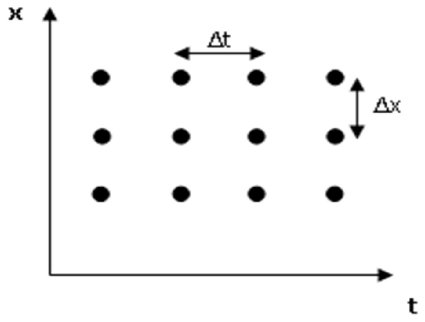
3. Finite Difference Approximations

The finite difference method is one of the many techniques to obtain numerical solutions of Equation (1). In all numerical solutions, the differential equation is replaced by a discrete approximation. In this context, the word “discrete” means that the numerical solution is known only at a finite number of points in the physical domain, see Figure 1. In general, increasing the number of points not only increases the resolution but also the accuracy of the numerical solution [36,37].
In many cases, it is not possible to find an analytical solution, especially with those real physical problems that have regions with non-regular geometry. However, convergence and stability tests ensure that the finite difference approximations used in the discretization are correct. There are ways to calculate the convergence of a code when the analytical solutions are known. Here, the parameters are taken into account to have a sufficiently fine mesh and thus obtain a convergent system in as few iterations as possible. To this end, we resort to the condition Δx ≤ k Δt, to ensure that the meshing is the one that best fits the solution space to be discretized. Knowing the value of Δx, the minimum number of nodes to give a numerical solution to this system can be determined. In this way, the central idea of the finite difference method is to replace continuous derivatives with so-called difference formulas involving only the discrete values associated with positions on the grid.
Applying the finite difference method to a differential equation involves replacing the derivatives with the corresponding finite difference expression, according to the appropriate scheme and accuracy. In the heat equation, there are derivatives concerning time and derivatives concerning space. Using different grids should confirm the stability of the solutions. In the limit when the mesh spacing (Δx and Δt) tends to zero, the numerical solution with either scheme will approach the true solution to the original differential equation, or the numerical solution approaches with less error to the true solution. However, how close the numerical solution approaches the true solution varies with the difference scheme used. Additionally, some practically useful schemes may fail to give a solution for bad combinations of Δx and Δt. This is what we want to verify in this work [38].
The discrete approximation results in a set of algebraic equations that are evaluated (or solved) for the values of the discrete variables. Figure 2 is a schematic representation of the numerical solution. The mesh is the set of points where the discrete solution is calculated (Figure 1). These points are called nodes; the lines between are adjacent to the domain nodes, and the resulting image would resemble a grid or mesh. The key parameters of the mesh are Δx, the local distance between adjacent points in space, and Δt, the local distance between adjacent time steps. For simplicity, the examples considered in this article Δx and Δt are uniform throughout the mesh.
The numerical solution of the heat equation is discussed in many textbooks. References [1,2,3,4,5,6,7,8] provide a more mathematical description of the development of finite difference methods. See Cooper [4] for a modern introduction to the theory of partial differential equations along with brief coverage of numerical methods [9,13,16] that takes a more applied approach and introduces implementation problems. Fletcher [4] provides development in Fortran for several methods.

4. Explicit Methods: Centered, Forward and Backward in Time Differences

The approximations to the governing differential equation are obtained by replacing all the continuous derivatives with discrete formulas such as those in Equation (3). The relationship between the continuous (exact) solution and the discrete approximation is shown in Figure 2 [38]. The finite-difference model is a distinct step of translating the continuous problem to the discrete one. The finite difference formulas are first developed with the dependent variable Ø as a function of a single independent variable, x, i.e., = x . The resulting formulas are then used to approximate derivatives concerning any space or time.

4.1. Direct Finite Difference of First Order

Consider a Taylor series expansion ϕ   x over the point.
ϕ   x i + δ x = x i + δ x
ϕ   x first order direct difference. Consider a Taylor series expansion ϕ   x over the point
ϕ xi   +   δ x = ϕ x i +   δ x ϕ x | x i + δ x 2 2   2 ϕ x 2 | x i + δ x 3 3 !   3 ϕ x 3 | x i +
where   δ x is a change in x to relative to x i . Let δ x = Δ x   in Equation (4), that is, consider the value at the location of the mesh line x i + 1 , i.e., x i + Δ x = x i + Δ x Note that the powers of multiply partial derivatives to the right-hand side have been reduced by one. The approximate solution is replaced by the exact solution, i.e., using i x i   y   i + 1 x i + Δ x
ϕ x | x i ϕ i + 1 ϕ i Δ x Δ x 2   2 ϕ x 2 | x i Δ x 3 3 !   3 ϕ x 3 | x i +
The mean value theorem can be used to replace the higher-order derivatives
ϕ x | x i ϕ i + 1 ϕ i Δ x + Δ x 2 2   2 ϕ x 2 | ε
or
ϕ x | x i ϕ i + 1 ϕ i Δ x Δ x 2 2     2 ϕ x 2 | ε
The term on the right-hand side of Equation (6) is called the truncation of the finite difference approximation. It is the error that results from truncating the series in Equation (5). In general, ξ is not known and is determined from the simulation. Although in the exact magnitude the truncation error cannot be known (unless the true solution Ø (x, t) is known analytically). The notation “Ο” can be used to express the dependence of the truncation error on the mesh spacing. The right-hand side of Equation (6) contains the mesh spacing Δx, which is selected for convenience.
The equal sign in this expression is true in the order of magnitude sense. That is, the O = Δ x 2 on the right-hand side of the expression is not strictly equal. Rather, the expression means that the left-hand side is a product of an unknown constant and Δx2. Although the expression does not give the exact magnitude of the error, it tells us how fast that term approaches zero as Δx becomes smaller. Using the notation Ο large, one can write Equation (5) as
ϕ x | x i = ϕ i + 1 ϕ i Δ x + Ο Δ x
The Equation (7) is known as the forward difference formula for x   x i because it involves x i   and   x i + 1 nodes. The forward difference approximation has a truncation error that is O (Δx). The size of the truncation error is under control because the mesh size Δx can be chosen.

4.1.1. First-Order Backward Difference

An alternative first-order finite difference formula is obtained if the Taylor series thus in Equation (4) is written with δx = −Δx. Using the discrete variable mesh instead of all unknowns, one obtains
    x | x i = ϕ i ϕ i + 1 Δ x + Ο Δ x
This is the backward difference formula because it involves the values of in x i   and   x i 1 (Figure 3). The order of magnitude of the truncation error for the backward difference presents an approximation equal to the direct difference approximation.
x i , t n + 1 x i , t n Δ t = d x i , t n + 1

4.1.2. First-Order Centered Difference

To obtain the centered finite difference approximation, we start from Equations (9) and (10), shown below:
  ϕ i + 1 = ϕ i + Δ x   ϕ x | x i + Δ x 2   2 ϕ x 2 | x i + ( Δ x ) 3 3 !   3 ϕ x 3 | x i +
ϕ i 1 = ϕ i Δ x   ϕ x | x i + Δ x 2   2 ϕ x 2 | x i ( Δ x ) 3 3 !   3 ϕ x 3 | x i +
By subtracting the results of Equation (10) from Equation (9)
ϕ x | x i = ϕ i + 1 ϕ i 1 2 Δ x + Ο Δ x 2
This is the centered difference approximation to x x i , the truncation error for approximation goes to zero much faster than the truncation error in Equation (7) or (8). There is a complication with Equation (11) because it does not include the value for i . This can cause problems when the centered difference approximation is included in an approximation to a differential equation.

4.1.3. Second-Order Centered Difference

Finite difference approximations to higher order derivatives can be obtained with the additional manipulations of the Taylor series expansion over x i . Adding the yields of Equations (9) and (10).
2 ϕ x 2 | x i = ϕ i + 1 2 ϕ i + ϕ i + 1 Δ   x 2 +   Ο Δ x 2
This is also called the central difference approximation, but (obviously) it is the approximation to the second derivative, while Equation (11) is the central difference approximation to the first derivative.
The finite-difference approximations developed above are now assembled into a discrete approximation to Equation (1). Both time and spatial derivatives are replaced by finite differences. Doing so requires specification of both the time and spatial locations of the Ø values in the finite-difference. Therefore, one needs to introduce the superscript m to designate the time of the discrete solution step. Although this seems to be only a simple problem, choosing the time step where the spatial derivatives are evaluated will have a great impact on the convergence and stability of finite difference implementation.

4.1.4. Difference Centered Forward in Time

Approximates the derivative of time in Equation (1) with a direct difference
ϕ t | t m + 1 ,       x i = ϕ i n + 1 ϕ i n Δ t + Ο Δ x
Implementation of the forward scheme (Figure 4) requires solving a system of equations at each time step. In addition to the complication of developing the code, the computational effort per time step for the backward scheme is greater than the computational effort per time step of the forward difference scheme. The forward scheme has a great advantage over the centered scheme: it is unconditionally stable (for solutions to the heat equation). Therefore, the forward scheme produces a robust computational model, even with the choice of Δt and Δx. This advantage, however, is not always appropriate and the centered scheme is still useful for some problems.
x i , t n + 1 x i , t n Δ t = d x i , t m

4.1.5. Implicit Method: Crank-Nicolson (CN)

In numerical analysis, the Crank-Nicolson (CN) method is a finite difference method used for the numerical solution of partial differential equations, such as the heat equation. It is a second order method in time, implicit and numerically stable.
For diffusive equations (and for many other types of equations), it can be shown that the CN method is unconditionally stable. However, the approximate solutions may still contain some spurious oscillations, depending on the relationship between the temporal and spatial spacings (Figure 5).
The FTSC and BTSC schemes have a truncation error in time of Ο (Δt). When very accurate solutions in time are needed, the CN scheme has significant advantages. The CN scheme is no more difficult to implement than the BTSC scheme, and has time truncation error of order Ο(Δt2). The CN scheme is implicit and stable [1,18,21]. The left-hand side of the heat equation is approximated differently from that used in the FTSC scheme. The right side of the heat equation is approximated by the average of the difference evaluated at the current and previous time.
Truncation errors in this order-of-magnitude approximation Ο (Δt2) + Ο (Δx2). In contrast to Equation (14), with Equation (15) the fact that it is not possible to rearrange to obtain an algebraic formula for n i in terms of its neighbors n , n   i + 1 , n   i 1 y n 1 (or simply adding 1 to each spatial subscript in Equation (15)) shows that n   i + 1 , depends on n   i + 2 , and n i . Thus, Equation (15) is a system of equations for the values of Ø at the internal nodes of the spatial grid (i = 2, 3, ..., N − 1).
x i , t n + 1 x i , t n Δ t = 1 2 d x i , t n + 1 + d x i , t m
The approximation error for the explicit schematic is O (Δt + Δx2) and the implicit Crack Nicolson scheme has an error of the order of O (Δt2 + Δx2). If the solution of the equation tends to the solution of the original differential equation when Δt → 0 and Δx → 0, the scheme in differences is convergent [1,4]. If the computational error produced at a certain time step decreases or at least does not increase when moving to the next time step, the scheme is stable.
For example, in the case of diffusion (l), the Crank-Nicolson discretization is:
1 m + 1 i m Δ t = α 2 Δ x 2 i + 1 m + 1 i m + 1 + i 1 m + 1 + i + 1 m i m + i 1 m
The Crank-Nicolson scheme is implicit, and one must solve a system of equations for the variable Ø at each time step. The system of equations is identical to transient problems in one spatial dimension, and the difference in computational cost is not significant. However, for transient problems with two or three spatial dimensions, the computational effort per forward time step is much larger than the computational effort per centered time step of difference. However, the stability is higher than forward. In problems in one, two, or three dimensions, CN generally provides a computational advantage [38].

4.1.6. The Algorithm

Figure 6 shows the algorithm for finding the numerical solution of the transfer equation.

4.1.7. Analytic Solution

By the method of separation of variables, if we assume that the solution Ø has the form Ø (x, t) = X (x). T(t) it reduces to a problem of ordinary differential equations with values on the boundary. Using classical methods for the solution of ordinary differential equations, we obtain the eigenvalues and the corresponding eigenfunctions that allow us to determine the expression of the analytical solution as a Fourier series given by
x , t = n = 1 b n e a n 2 π 2 L 2   t s i n n π L   x
where b n with n ∈ N are the coefficients of the Fourier series development of the function f(x) (initial condition of the problem) and are determined by the formula
b n = 2 L 0 L f x s i n n π L x d x
With the appropriate boundary conditions the analytical solution Ø (x, t) is obtained [39,40].

5. Results

5.1. Numerical Implementation

The finite difference method allows us to obtain an approximate solution for Ø (x, t) at a finite set of points x and t for the codes developed in this paper. There are plausible schemes that do not exhibit this important property of converging to the true solution. See the consistency discussions in references [1,4]. The numerical implementation is performed uniformly spaced in the interval 0 ≤ x ≤ L such that x i = i 1 Δ x ,   i = 1 , 2 , 3 N where is the total number of spatial nodes, including those on the edge. Given L and N, the space between x i is calculated with Δx = L/(N − 1). Similarly, the discrete times are uniformly spaced in 0 t t m a x : t m = m 1 Δ t ,   m = 1 , 2 , .. M where M is the maximum number of time steps and Δt is the size of a time step ∆t = t m a x / M 1 .

5.2. Estimates of Truncation Error (TE)

The TE for the centered or forward schemes is O (Δt) + O (Δx2). The notation O large expresses the rate at which the TE reaches zero. For code validation, we worked with the magnitude of the TE. For a Δt, Δx given as Δt → 0 and Δt → 0, the true magnitude of the truncation error is [41,42,43,44,45,46]
T E = K t Δ t + K x Δ x 2
where K t y K x are constants that depend on the accuracy of the finite-difference approximations implemented. To make TE arbitrarily small, both Δt and Δx must approach zero. To verify that an FTSC or BTSC (results are shown in Figure 7, Figure 8 and Figure 9) code works correctly, we wish to determine whether a reduction in Δt causes a reduction in TE.
Similarly, if one wishes to determine whether a linear reduction in Δx causes a quadratic reduction in TE, one must vary only Δt or Δx. The NC scheme shows a quadratic reduction in TE with Δt (Figure 10).
One could also use the second-order L1 rules norm, comparing the numerical solution with the analytical one to determine the error at the level of approximation, as expected.
Figure 11 shows the pseudocode used for the analysis of the heat equation.

5.3. Solutions Validation

To verify the built-in algorithm, problems that have exact solution are solved and the analytical results are compared with the numerical solution of the code. A proposed example is a 3 m long thin wire, and the material properties are: k = 12 w/m°K.
Table 1 shows the analytical and approximate results of the solution of the one-dimensional problem given as an example, with an approximation of two decimal digits. It shows the accuracy that the computer code can achieve when solving the finite difference problem using the FTCS, CN, and BTCS methods, respectively.

5.4. Discussion

When performing simulations involving numerical solutions of partial differential equations, it is evident that, apart from rounding and series truncation errors (recall that finite difference expressions are derived from a Taylor series development up to second-order), there are the errors inherent in the limitations of fitting the physical model to accurately describe the real physical system and the limitations of the boundary conditions [47,48,49,50].
The numerical time integration of the equations can be done explicitly or implicitly. In the former, its main advantage is the possibility to solve each time step, without the need to solve a system of equations where all the degrees of freedom are involved. Its disadvantage is the stability of the solutions, which in many cases leads to time steps that are too small to be efficient.
On the contrary, implicit methods allow, under certain conditions, always stable time steps, whose size must be regulated only by criteria of precision and not of stability. In return, a system of equations involving all of its degrees of freedom must be solved, which makes the method costly and difficult to parallelize.
The implicit method is the Crank-Nicholson method, it has an order of approximation equal to Ο (Δt2 + Δx2). This method has the advantage of being unconditionally stable, i.e., the instability phenomenon does not appear in the solution that was seen for the explicit method. Figure 6 shows the temperature profile achieved under the conditions that introduced instability in the explicit scheme, that is, for Δx = 5/13 and Δt = 0.5.
Figure 7, Figure 8 and Figure 9 show the temperature profiles for the three discretization schemes presented in this work. CN outperforms the FTCS and BTCS schemes in terms of stability, convergence, and smoothness of the solutions.
Table 1 compares the values achieved using the three schemes with the analytical solution. As can be seen in them and as mentioned, a better approximation is achieved for CN, compared to FTCS and BTCS.
To study stability it is sufficient that the solutions of the differential equations do not present oscillations (are regular), even more so when the solutions are time-dependent. It is necessary to let the time-dependent variables evolve for a long time to verify that they do not present oscillations or irregular peaks, as can be seen in Figure 6.
All the runs of the codes were elaborated with the three schemes. A mesh refinement was performed to verify the stability of the solutions. These discretization schemes can be extended to 2D and 3D problems.
In some cases when the analytical solution is not known, one way to perform convergence is to take the numerical value of the first iteration of the program as the analytical solution and compare it with the numerical value of the second iteration. Then, the value of the second iteration is taken as the analytical solution and compared with the numerical value of the third iteration and so on. The convergence consists of checking how close the numerical solution obtained is to a known analytical solution.
To perform the convergence of the code elaborated in FORTRAN77, we proceeded as follows: since the finite difference approximation method used in the Taylor series development is of second order, it is postulated that the error is also of second order in ∆x. Plotting log (error) Vs log (∆x) (where error involves the numerical and analytical solution), the error between a known analytical solution and the numerical solution found for the heat equation is obtained. A slope approximately equal to two implies that the numerical solution converges to the analytical solution. In this case, a general expression for convergence calculation given by the L1 rules [20], where f i j is the analytical solution and F i j   is the numerical solution obtained and L1 = Error, was used for convergence.
The results obtained for each method used were of 1.7 (BTCS), 1.8 (FTCS), and 2.0 with CN, in full agreement with those expected by the second-order approximation error.
From the above, it is established that the errors found showed a tendency for the NC method to better approximate the analytical solution in terms of error and convergence in most of the tests performed.

6. Conclusions

This work serves as a preamble to more complex problems such as the application of the 1D heat equation in the area of finance. Using as motivation a simple example of application of the diffusion equation, it has been possible to compare the application of different methods for its solution. Explicit and implicit numerical methods were presented with their advantages and disadvantages in terms of the stability of each one. The user can select the solution method according to the required needs. That is, noticing the instability problem, the desired method can be selected by choosing the length of the spatial and temporal interval.
It can be seen that the application of an implicit method allows one to obtain the solution without falling into the instability phenomenon. Additionally, the Crank-Nicholson method allows for better approximation. However, there are cases in which such a strict approximation error may not be necessary; in such cases, an explicit method with fewer calculations but taking care of the stability of the scheme will suffice.
The mathematical formulation with CN and Dirichlet conditions [34] is the most appropriate for the solution in the three cases shown. This was verified using Newman conditions in the three schemes used. This model represents an important tool in the design and optimization of the processes, so much so that it can be used to test new experimental conditions, aiming at the decrease of time and costs involved in the simulation of the heat transfer equation in different physical systems.
There are many finite difference schemes for solving differential equations. It is numerical experimentation that reveals which of the different schemes is the best to use. The important factor is to see whether the equations are parabolic, elliptic, or hyperbolic; one scheme may be more appropriate than others when performing stability and convergence of the solutions.
To verify the results, a series of simulations previously performed by other authors [1] is carried out to induce a thorough understanding of the heat transfer phenomena, always keeping a critical attitude towards the program that executes the calculations. It is time to integrate partial differential equations and simulations to understand that simulations require as much or more time than an experimentalist in a laboratory to demonstrate the veracity, validity, and strengths of the same and contribute to establishing the paradigms of all the aspects that accompany a simulation. All the cases were solved with FORTRAN 77. In several cases, the capabilities of the program developed with FORTRAN 77 were reached in terms of meshes and calculation times.

Author Contributions

Conceptualization, F.S.-C. and L.R.-R.; methodology, F.S.-C. and L.R.-R.; investigation, F.S.-C. and L.R.-R.; writing—original draft preparation L.R-R.; writing—review and editing F.S.-C.; supervision, F.S.-C. and L.R.-R.; project administration, F.S.-C. and L.R.-R. Both authors have read and agreed to the published version of the manuscript.

Funding

This research was funded by Universidad de Las Américas-Ecuador and Universidad Politécnica de Venezuela, Puerto Ordaz.

Institutional Review Board Statement

Not applicable.

Informed Consent Statement

Not applicable.

Data Availability Statement

The data has not been published in any other journal or any other place of publication. However, they are available at the UNEXPO Physics Laboratory, Puerto Ordaz, Venezuela.

Conflicts of Interest

The authors declare no conflict of interest.

References

  1. Ames, W. Numerical Methods for Partial Differential Equations; Academic Press, Inc.: Boston, MA, USA, 1992. [Google Scholar]
  2. Olsen-Kettle, L. Numerical Solution of Partial Differential Equations and Code; Swinburne University of Technology: Melbourne, Australia, 2011; pp. 14–28. [Google Scholar]
  3. Adak, M. Comparison of Explicit and Implicit Finite Difference Schemes on Diffusion Equation. In Mathematical Modeling and Computational Tools ICACM 2018. Springer Proceedings in Mathematics & Statistics; Bhattacharyya, S., Kumar, J., Ghoshal, K., Eds.; Springer: Singapore, 2018; Volume 320. [Google Scholar]
  4. Cooper, J. Introductin to Partial Differential Equations with Matlab; Birkhuser: Boston, MA, USA, 1998. [Google Scholar]
  5. Sequeira-Chavarría, F.; Ramírez-Bogantes, M. Computational Aspects of the Finite Difference Method for the Time-Dependent Heat Equation. Uniciencia 2019, 33, 83–100. [Google Scholar] [CrossRef] [Green Version]
  6. Morton, K.W.; Mayers, D.F. Numerical Solution of Partial Differential Equations: An Introduction; Cambridge University Press: Cambridge, UK, 1994. [Google Scholar]
  7. Chapra, S.C.; Canale, R.P. Métodos Numéricos Para Ingenieros; McGraw-Hill/Interamericana Editores: New York, NY, USA, 2007. [Google Scholar]
  8. Millán, Z.; de la Torre, L.; Oliva, L.; Berenguer, M. Simulación numérica: Ecuación de difusión. Rev. Iberoam. Ing. Mecánica 2011, 15, 29–38. [Google Scholar]
  9. Fletcher, C. Computational Techniquess for Fluid Dynamics; Springer: Berlin, Germany, 1998. [Google Scholar]
  10. Khan, M.N.; Ahmad, I.; Akgül, A.; Ahmad, H.; Thounthong, P. Numerical solution of time-fractional coupled Korteweg–de Vries and Klein–Gordon equations by local meshless method. Pramana J. Phys. 2021, 95, 6. [Google Scholar] [CrossRef]
  11. Liu, C.; Liu, X.; Yang, Z.; Yang, H.; Huang, J. New stability results of generalized impulsive functional differential equations. Sci. China Inf. Sci. 2021, 65, 129201(2022). [Google Scholar] [CrossRef]
  12. Recktenwald, G. Finite-Difference Approximations to the Heat Equation. Mech. Eng. 2011, 10, 4–20. [Google Scholar]
  13. Golub, G.; Ortega, J. Scientific Computing: An Introduction with Parallel Computing; Academic Press, Inc.: Boston, UK, 1993. [Google Scholar]
  14. Camacho, A.; Guardian, B.; Jacobo, V.; Ortiz, A. El método alternativo de Schwarz y la computación paralela. In Proceedings of the MEMORIAS XXIV Congreso Internacional Anual de la SOMIM, Campeche, Mexico, 19–21 September 2018; pp. 77–82. [Google Scholar]
  15. Huang, J.; Nualart, D.; Viitasaari, L. A central limit theorem for the stochastic heat equation. Stoch. Process. Appl. 2020, 130, 7170–7184. [Google Scholar] [CrossRef]
  16. Hoffman, J. Numerical Methods for Engineers and Scientists; McGraw-Hill: New York, NY, USA, 1992. [Google Scholar]
  17. O’Neil, P. Matemáticas Avanzadas Para Ingeniería, 7th ed.; Cengage Learning: Boston, MA, USA, 2015. [Google Scholar]
  18. Ibarra, M.C. La ecuación de calor de Fourier: Resolución mediante métodos de análisis en variable real y en variable compleja. In UTN Facultad Regional Resistencia: II Jornadas de Investigación en Ingeniería del NEA y Países Limítrofes; Universidad Técnica Nacional: Misiones, Argentina, 2012. [Google Scholar]
  19. Mamani Condori, F.; Gonzales Medina, R. Aplicación de Las Series de Fourier en la Solución de Problemas Con Valor Inicial en la Frontera. Veritas 2019, 13, 225–230. [Google Scholar]
  20. Cranmer, K.; Brehmer, J.; Louppe, G. The frontier of simulation-based inference. Proc. Natl. Acad. Sci. USA 2020, 117, 30055–30062. [Google Scholar] [CrossRef]
  21. Cannon, J. The One-Dimensional Heat Equation, Encyclopedia of Mathematics and Its Applications; Cambridge University Press: Cambridge, UK, 1984. [Google Scholar]
  22. Martín-Vaquero, J.; Vigo-Aguiar, J. On the numerical solution of the heat conduction equations subject to nonlocal conditions. Appl. Numer. Math. 2009, 59, 2507–2514. [Google Scholar] [CrossRef]
  23. Li, Y. Central limit theorem for a fractional stochastic heat equation with spatially correlated noise. Adv. Differ. Equ. 2020, 1–9. [Google Scholar] [CrossRef] [Green Version]
  24. Madera, S.; Ortega-Quitana, F.; Lopez, A.; Perez, O. Determinación del Coeficiente Convectivo de Transferencia de Calor del Proceso de Escaldado de Zapallo (Cucurbita maxima). Inf. Tecnol. 2017, 28, 59–66. [Google Scholar] [CrossRef] [Green Version]
  25. Meza Castro, I.F.; Herrera Acuña, A.E.; Obregón Quiñones, L.G. Determinación Experimental de Nuevas Correlaciones Estadísticas para el Cálculo del Coeficiente de Transferencia de Calor por Convección para Placa Plana, Cilindros y Bancos de Tubos. INGE CUC 2017, 13, 9–17. [Google Scholar] [CrossRef] [Green Version]
  26. Isaacson, E.; Keller, H.B. Analysis of Numerical Methods; Dover Books on Mathematics: New York, NY, USA, 1994. [Google Scholar]
  27. Skiba, Y.; Métodos, Y. Esquemas Numéricos: Un Análisis Computacional. In Dirección General de Publicaciones Y Fomento Editorial; Universidad Autónoma de México: Mexico City, Mexico, 2005. [Google Scholar]
  28. Mathews, J.H.; Fink, D.F. Métodos Numéricos con MATLAB; Prentice-Hall: Madrid, España, 2000. [Google Scholar]
  29. Caligaris, M.G.; Rodríguez, G.; Favieri, A.; Laugero, L. Desarrollo De Habilidades matemáticas Durante La resolución numérica De Problemas De Valor Inicial Usando Recursos tecnológicos. Rev. Digit. Educ. Ing. 2019, 14, 30–40. [Google Scholar] [CrossRef] [Green Version]
  30. Duarte, P.; Cristianini, M. Determining the Convective Heat Transfer Coefficient (h) in Thermal Process of Foods. Int. J. Food Eng. 2011, 7, 56–68. [Google Scholar]
  31. Zhukovsky, K.V.; Srivastava, H.M. Analytical solutions for heat diffusion beyond Fourier law. App. Maths Comp. 2017, 293, 423–437. [Google Scholar] [CrossRef]
  32. Hou, Q.; Lin, T.-C.; Wang, Z.-A. On a singularly perturbed semi-linear problem with robin boundary conditions. Disc. Cont. Dyna. Sys. Ser. B 2021, 26, 401–414. [Google Scholar] [CrossRef] [Green Version]
  33. Degond, P.; Génieys, S.; Jüngel, A. A steady-state system in non-equilibrium thermodynamics including thermal and electrical effects. Math. Meth. Appl. Sci. 1998, 21, 1399–1413. [Google Scholar] [CrossRef]
  34. Shi, J.; Jiang, F. On Neumann problem for the degenerate Monge–Ampère type equations. Bound Value Probl. 2021, 11. [Google Scholar] [CrossRef]
  35. Sadybekov, M.A.; Torebek, B.T.; Turmetov, B.K. Representation of the Green’s function of the exterior Neumann problem for the Laplace operator. Sib. Math. J. 2017, 58, 153–158. [Google Scholar] [CrossRef]
  36. Kreyszig, E. Advanced Engineering Mathematics; John Wiley & Sons: New York, NY, USA, 2011. [Google Scholar]
  37. Zill, D. Advanced Engineering Mathematics; Jones & Bartlett Learning: Burlington, MA, USA, 2018. [Google Scholar]
  38. Salazar, J.; Rosales, L. Simulación de la ecuación de conducción del calor en el proceso de ensamblaje de un sistema rotativo. In Memorias de las IX Jornadas de Investigación; UNEXPO: Puerto Ordaz, Venezuela, 2011; pp. 249–253. [Google Scholar]
  39. Perussello, C. Heat and mass transfer modeling of the osmo-convective drying of yacon roots. Appl. Therm. Eng. 2014, 63, 23–32. [Google Scholar] [CrossRef]
  40. Al-Zareer, M.; Dincer, I.; Rosen, M.A. Heat and mass transfer modeling and assessment of a new battery cooling system. Int. J. Heat Mass Transf. 2018, 126, 765–778. [Google Scholar] [CrossRef]
  41. Burden, R.L.; Faires, J.D. Numerical Analysis; Brooks/Cole Publishing Co.: New York, NY, USA, 1997. [Google Scholar]
  42. Nikan, O.; Jafari, H.; Golbabai, A. Numerical analysis of the fractional evolution model for heat flow in materials with memory. Alex. Eng. J. 2020, 59, 2627–2637. [Google Scholar] [CrossRef]
  43. Akbaş, Ş. Nonlinear static analysis of laminated composite beams under hygro-thermal effect. Struct. Eng. Mech. 2019, 72, 433–441. [Google Scholar] [CrossRef]
  44. Tinoco, H.A. Análisis del Efecto Termo-Elástico Como Inductor de Vibraciones en Rodamientos, Trabajo de Grado; Universidad Autónoma de Manizales, Facultad de Ingeniería, Programa de Ingeniería Mecánica: Caldas, Colombia, 2004; pp. 100–105. [Google Scholar]
  45. Chen, H.; Lin, S.; Xiong, C. Analysis and Modeling of Thermal Effect and Optical Characteristic of LED Systems with Parallel Plate-Fin Heatsink. IEEE Photonics J. 2017, 9, 1–11. [Google Scholar] [CrossRef]
  46. Agudelo, A.; Gónzalez, L.J. Ecuación Diferencial Asociada a los Polinomios Ortogonales Clásicos. Sci. Tech. 2004, 10, 179–184. [Google Scholar]
  47. Guo, Y.; Cao, X.; Liu, B.; Gao, M. Solving Partial Differential Equations Using Deep Learning and Physical Constraints. Appl. Sci. 2020, 10, 5917. [Google Scholar] [CrossRef]
  48. Zwarycz-Makles, K.; Majorkowska-Mech, D.; Runge-Kutta, G. Numerical Discretization Methods in Differential Equations of Adsorption in Adsorption Heat Pump. Appl. Sci. 2018, 8, 2437. [Google Scholar] [CrossRef] [Green Version]
  49. Lim, S.; Koo, M.-S.; Kwon, I.-H.; Park, S. Model Error Representation Using the Stochastically Perturbed Hybrid Physical–Dynamical Tendencies in Ensemble Data Assimilation System. Appl. Sci. 2020, 10, 9010. [Google Scholar] [CrossRef]
  50. Lipp, V.; Rethfeld, B.; García, M.; Ivanov, D. Solving a System of Differential Equations Containing a Diffusion Equation with Nonlinear Terms on the Example of Laser Heating in Silicon. Appl. Sci. 2020, 10, 1853. [Google Scholar] [CrossRef] [Green Version]
Figure 1. For the sake of generality, the discretization scheme is shown with the spacings in time and space.
Applsci 11 04468 g001
Figure 2. Relationship between the continuous problem and the discrete problem.
Applsci 11 04468 g002
Figure 3. Finite difference backward in time (BTCS). Known values are indicated with black circles and unknown values with a white circle.
Applsci 11 04468 g003
Figure 4. Finite forward difference (FTSC). Unknown values are indicated with a black circle and known values with white circles.
Applsci 11 04468 g004
Figure 5. Crank-Nicolson scheme. Unknown values are indicated with black circles and known values with white circles.
Applsci 11 04468 g005
Figure 6. Algorithm for the numerical solution.
Applsci 11 04468 g006
Figure 7. Evolution of the temperature in the thin bar versus time and using finite difference backward (BTCS). The instability of the solution is remarkable.
Applsci 11 04468 g007
Figure 8. Evolution of the temperature on the thin bar as a function of time and position for a grid of 100,000 points on the spatial grid using FTCS.
Applsci 11 04468 g008
Figure 9. Evolution of bar temperature versus time and bar point position for a mesh of 150,000 points on the spatial grid using backward finite differences (BTCS).
Applsci 11 04468 g009
Figure 10. Evolution of bar temperature versus time and bar point position for a mesh of 150,000 points on the spatial grid using Crank-Nicolson (CN).
Applsci 11 04468 g010
Figure 11. Pseudo code showing the numerical scheme in FORTRAN 77 implemented with finite difference for the heat equation.
Applsci 11 04468 g011
Table 1. Comparison of the exact (analytical) and approximate (numerical with forward difference, FTCS, CN, and BTCS) solution of the example.
X(m)Analytical Temperature (°C)Numerical Temperature
(FTCS) (°C)
Numerical Temperature (CN) (°C)Numerical Temperature (BTCS) (°C)
050.0050.0050.0050.00
0.5125.10124.76125.21120.23
1.0154.32154.79154.02150.33
1.5175.22176.43175.13169.07
2.0202.37204.84202.34199.97
2.5225.12225.75225.18221.86
3.0167.35166.13167.27163.45
Publisher’s Note: MDPI stays neutral with regard to jurisdictional claims in published maps and institutional affiliations.

