Serial Detection with Neural Network-Based Noise Prediction for Bit-Patterned Media Recording Systems

Abstract

Ultra-high density data storage has gained high significance given the increasing amounts of data; many technologies have been proposed to achieve a high density. Among them, bit-pattern media recording (BPMR) is a promising technology. In BPMR systems, data are stored on magnetic islands. Therefore, high densities can be achieved by reducing the distance between the magnetic islands. Because of the closeness between the magnetic islands, the readback signal is distorted by two-dimensional (2D) interference, which includes the intersymbol interference according to the down-track direction and the intertrack interference according to the cross-track direction. A simple and effective serial detection algorithm was recently proposed to mitigate the 2D interference. However, serial detection utilizes the hard output in inner detection, and this degrades the serial detection performance. To resolve this problem, a subsequent study used feedback to estimate the noise and used this noise signal to create a soft output for inner detection. Following up, in this paper we propose a model that utilizes a neural network for noise prediction. The proposed neural network-based model and the model with the feedback line were compared in terms of bit error rate (BER). The results show that the proposed model achieves a gain of approximately 1 dB at a BER of 10⁻⁶.

1. Introduction

Currently, the rapid development in data science has led to an ever-increasing amount of data. Therefore, the demand for data storage has accordingly increased. Storage technologies are of two types, namely solid-state storage and magnetic storage. In solid-state storage, the data are stored as electrons in floating gates [1], whereas in magnetic storage, the data are magnetized and stored in a magnetized medium [2]. The choice between solid-state storage and magnetic storage involves a trade-off between reading speed and cost per bit [3].

The initial recording medium was a magnetic material with many randomly oriented magnetic grains. Therefore, it is limited to an areal density (AD) of approximately 1 Tb/in² by superparamagnetic phenomena [4]. To overcome this problem, several new technologies have been proposed, including heat-assisted magnetic recording (HAMR) [5], two-dimensional (2D) magnetic recording (TDMR) [2], and bit-patterned media recording (BPMR) [6]. Among these, BPMR is a promising candidate for future technology.

For BPMR, the recording media structure is based on magnetic islands surrounded by nonmagnetic zones. To increase the AD, we need to reduce the area of the nonmagnetic region, thus making the magnetic islands closer. However, with closer distances, BPMR experiences more two-dimensional (2D) interference. The 2D interference consists of intersymbol interference (ISI) and intertrack interference (ITI) upon reducing the distance according to the down-track and cross-track directions, respectively. Furthermore, BPMR suffers from track misregistration (TMR) and media noise [7,8].

Many signal-processing algorithms have been proposed to address 2D interference. Typically, there are two common approaches, namely symbol detection methods and error-correcting or/and modulation coding methods. The key concept behind the modulation codes is that the symbols must not be surrounded by the opposite polarity symbols to prevent 2D interference. However, these symbols can have room for error correction if the minimum distance of the code is greater than one. To reduce the ITI, Buajong and Warisarn [9] designed a rate 3/4 modulation code that subtracts the ITI. Based on the staggered BPMR, Nguyen and Lee proposed an error-correcting 5/6 modulation code to reduce the isolated bit and correct the errors [10]. Jeong and Lee [11] introduced a modulation code and its multilayer perceptron decoding for BPMR to reduce and correct the errors by the ITI.

For symbol detection, maximum likelihood (ML) detection and maximum a priori (MAP) detection are commonly used for white noise and colored noise channels, respectively. The Viterbi algorithm (VA) and Bahl–Cocke–Jelinek–Raviv (BCJR) algorithms are representative of ML and MAP detections, respectively. In principle, the Viterbi and BCJR algorithms are designed to remove 1D interference, such as the ISI. However, in the BPMR, the signal suffers from 2D interference; therefore, we need to modify Viterbi and BCJR to be suitable for 2D interference. Nabavi and Kumar [12] proposed a model that includes a 2D equalizer and a generalized partial response (GPR) target to estimate the interference. Consequently, the interference value is applied for detection to efficiently remove the interference in the signal. In addition, Nabavi et al. introduced a modified Viterbi algorithm (MVA) to supply ITI information for the VA [13]. Thus, MVA can reduce the ITI and improve the BER performance of BPMR systems. In addition to the improvements in [12,13], Wang and Kumar combined GPR and MVA to enhance the channel estimation when the ITI characteristic is known, and the method is referred to as a hybrid 2D equalizer [14]. Further, to mitigate 2D interference, Kim and Lee [15] suggested a 2D soft-output VA (2D SOVA). In 2D SOVA, the received signal is detected in parallel by two 1D Viterbi detectors applied in the horizontal and vertical directions, respectively. Initially, the 2D SOVA was developed for holographic data storage systems; however, Kim et al. proposed an iterative 2D SOVA for bit-patterned media [16]. Because 2D SOVA takes the received signal through two 1D detectors, the complexity is similar to the VA, and it fits 2D interference. Recently, Jeong and Lee improved the 2D SOVA into a multipath ISI structure that is suitable for a staggered BPMR structure [17].

In addition to parallel detection, serial detection for BPMR was also proposed by Nguyen and Lee [18]. In serial detection, GPR is decomposed into a series of two (down-track and cross-track) 1D PR targets to estimate the 2D interference. Based on the serial form of the GPR, serial detection that includes two serial 1D Viterbi detectors is proposed. The first detector is used for inner detection, using the VA to convert the received signal into a six-level signal. This implies that the inner detection still detects the signal in the hard output, which reduces the performance of serial detection. Therefore, Nguyen and Lee [19] resolved this problem using a soft output for inner detection in serial detection. To create a soft output, the noise information is estimated from the received signal, and then added to the hard output of the inner detection.

In addition to the VA, there are many detection schemes based on the BCJR algorithm. Cheng et al. proposed an iterative row-column soft decision feedback algorithm (IRCSDFA) to address the 2D interference [20]. Because Cheng et al. considers the 2D input in the trellis, IRCSDFA is similar to 2D detection; however, the complexity of IRCSDFA is extremely high. Subsequently, Zheng et al. proposed a less complex IRCSDFA applying Gaussian approximation (IRCSDFA-GA) [21]. Although IRCSDFA-GA has low-complexity compared to IRCSDFA, it is still more complex than the VA.

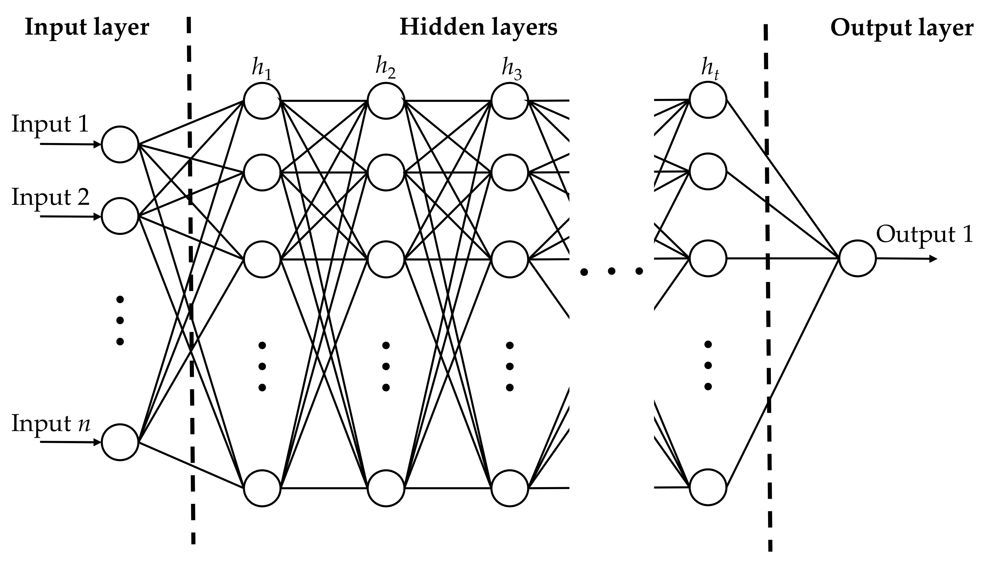
In recent years, the neural network approach has been extensively studied and widely applied to symbol detection. In the field of communication, neural networks are used as nonlinear equalizers having a higher performance capacity compared to the linear equalizer [22]. Further, in data storage, the neural networks can replace the equalizer and improve the performance compared to the conventional equalizer [23]. In [24], the detection scheme using a neural network coupled with TMR predicting ability achieved better performance than partial response maximum likelihood (PRML) detection. For the modulation code, Jeong showed that a decoder using a neural network outperformed a decoder with a minimum Euclidean distance [25].

In this study, based on the concepts in [19] and the wide application of neural networks in data storage systems, we built a model using a neural network to predict the noise information for the soft output in serial detection. However, when the neural network is trained at a low noise level, it does not satisfactorily predict the noise because of overfitting. Therefore, we designed a noise power estimator to reduce the overfitting. The proposed model includes two parts––one predicting the distortion of the noise using the neural network, and the other estimating the noise power using a parameter that is multiplied by the predicted noise. We also compared the proposed model with the model in [19]. The results show that our model achieves a better BER performance than the soft output model in [19].

The remainder of this paper is organized as follows. The serial detection and theory of the proposed model are described in Section 2. The proposed model is explained in Section 3. In addition, we also compare our model with the soft output model in [19]. The results and discussion are presented in Section 4. Finally, in Section 5, the conclusions are presented.

2. Serial Detection

This section details the proposed serial detection method and discusses the use of soft output to improve serial detection. Further, an example to elucidate the hard and soft outputs is presented.

2.1. GPR Target and Serial Detection

Our model applies the GPR target in [18] to create a serial detection. The proposed system consists of two processes, namely training and testing. The interference coefficients of the GPR target were estimated during the training process as in [18], with the minimum mean square error (MMSE) algorithm. In (1), the difference between the estimated signal z[j,k] and the desired signal d[j,k] is defined as e[j,k]. The signal e[j,k] is squared and minimized to determine the optimal coefficients r and p in the target G.

$$\underset{F\mathrm{and}G}{\arg \min }\left(E\left\{e{[j,k]}^2\right\}\right)=\underset{F\mathrm{and}G}{\arg \min }\left(E\left\{{\left(z[j,k]-d[j,k]\right)}^2\right\}\right),$$

(1)

where d[j,k] = a[j,k]*G, such that a[j,k] ∈ {−1, 1} and

$$G=\left[\begin{array}{ccc}rp& p& rp\\ r& 1& r\\ rp& p& rp\end{array}\right]=\left[\begin{array}{c}p\\ 1\\ p\end{array}\right]\ast \left[\begin{array}{ccc}r& 1& r\end{array}\right]\mathrm{a}=1,$$

(2)

The solution of (1) is presented in Section 3. Here, we consider the form of the target G, which includes the 2D interferences in the horizontal and vertical directions. These interferences can be decomposed in a serial form. Therefore, in [18], the authors implemented a serial detection scheme that removed the horizontal interference first, followed by vertical interference. The serial detection model is illustrated in Figure 1.

2.2. Soft Output for Serial Detection

To improve the serial detection, in [19], the authors added the noise information to the signal s[j,k] and created a soft output. To explain this, we consider a simple example. Assume that the data have two bits x = [x[0] x[1]]^T; x[k] ∈ {−1, 1}, that is, x ∈ {−1, 1} × {−1, 1}, and the channel interference is [0.2 1 0.2]. Based on the trellis diagram in Figure 2 with the starting status [−1 −1], we have the channel interfered signal z as in

Table 1. The values z corresponding to the values x.

x	z
[−1 −1]	[−1.4 −1.4]
[−1 1]	[−1.4 −1]
[1 −1]	[−1 0.6]
[1 1]	[−1 −1]

. In Figure 2, the dashed line represents assigning input 1, and the solid line represents assigning input −1.

If the original signal x is [1 −1]^T, the noise e is [0.1017 0.4458]^T. The received signal z_e is [−0.8983 1.0458]^T, calculated using (3) and (4). y_e is decoded using the VA, and the trellis diagram is shown in Figure 3.

$$z=x*{[\begin{array}{ccc}r& 1& r\end{array}]}^T,$$

(3)

$$z_e=z+e,$$

(4)

In Figure 3, we can observe that the path with metric (0.1017, 0.0458) is the maximum likelihood path. Therefore, the detected result is [1 1]^T.

Further, it is known that VA finds the sequence values z, which is similar to the received sequence z_e. This is represented in the formula as follows:

$$\underset{z[k]}{\mathrm{argmin}}{\displaystyle \sum _{k=0}^{L-1}{(z_e[k]-z[k])}^2},$$

(5)

where L is the number of bits of the data sequence, and z[k] is the output of the paths in the trellis. Usually, the output of the detector is a hard (discrete value) output. However, if this result is used in serial processing, the next detection process has no margin to correct the result because the signal [1 1]^T is a right vector. Thus, to correct this result in the next detector, we should add the noise (i.e., interference) information to create a soft (continuous value) output.

We propose a neural network to predict the noise vector e that is supplied for serial detection to create the soft output after the inner detection. In the next section, we investigate the structure of the neural network suitable for predicting the noise vector e from z_e.

2.3. Neural Network

In Figure 4, the structure of the neural network is fully connected and includes n inputs, t hidden layers having h_t neurons for each layer, and 1 output neuron. Thus, the structure of the neural network can be defined by selecting the parameters n, t, and h_t. Let h = [h₁ h₂ h₃ … h_t] correspond to the hidden layers. For instance, if h = [90 42 53], we have 90, 42, and 53 neurons for the first, second, and third hidden layers, respectively. For the input of the neural network, we consider a block of size 5 × 5 and a vector of size 25 × 1, as in Equations (6) and (7), respectively [24].

$$Y_{nn}=\left[\begin{array}{ccccc}y[j-2,k-2]& y[j-2,k-1]& y[j-2,k]& y[j-2,k+1]& y[j-2,k+2]\\ y[j-1,k-2]& y[j-1,k-1]& y[j-1,k]& y[j-1,k+1]& y[j-1,k+2]\\ y[j,k-2]& y[j,k-1]& y[j,k]& y[j,k+1]& y[j,k+2]\\ y[j+1,k-2]& y[j+1,k-1]& y[j+1,k]& y[j+1,k+1]& y[j+1,k+2]\\ y[j+2,k-2]& y[j+2,k-1]& y[j+2,k]& y[j+2,k+1]& y[j+2,k+2]\end{array}\right],$$

(6)

$$y_{nn}={\left[\begin{array}{cccccc}y[j-2,k-2]& \dots & y[j-2,k+2]& y[j-1,k-2]& \dots & y[j+2,k+2]\end{array}\right]}^T,$$

(7)

Hence, there are 25 inputs (i.e., n = 25) and one output neuron. As regards the structure of the hidden layer, many studies have suggested optimal numbers of hidden layers and neurons; however, no universally accepted method exists for a particular problem [26]. Therefore, using the model in Figure 5 for training, we used the mean square error (MSE) parameter to experimentally evaluate the structure of the hidden layers.

The details of the model are described in the next section. In Figure 5, the training process of the neural network is illustrated. In the training process, we implement it as in [22,24]. We collect a data block size of 5 × 5 including two neighboring ISI and ITI bits for all eight directions from y[j,k] and reshape that into a size of 25 × 1 for the input of the neural network. The noise signal e[j,k] is the label for the output of the neural network, which is the difference between z[j,k] and d[j,k] after estimating the parameter of the GPR target. The estimation of the GPR target was performed before training the neural network. In addition, we used the scaled conjugate gradient (SCG) algorithm [27] to optimize the network parameters.

Table 2. MSE of the neural network with one hidden layer.

Hidden Layer	MSE
[5]	0.0442
[10]	0.0425
[20]	0.0302
[50]	0.0273
[100]	0.0272
[200]	0.0475

,

Table 3. MSE of the neural network with two hidden layers.

Hidden Layer	MSE
[40 60]	0.0182
[50 50]	0.0178
[60 40]	0.0168
[20 80]	0.0179
[100 100]	0.0186
[80 20]	0.0197

and

Table 4. MSE of the neural network with three hidden layers.

Hidden Layer	MSE
[30 20 50]	0.0238
[50 50 50]	0.0171
[50 20 30]	0.0162
[20 50 30]	0.0154
[30 50 20]	0.0141
[20 30 50]	0.0169

show the resulting MSEs for each structure. For reasonable complexity, we tested one to three hidden layers and approximately 100 neurons. In addition, when increasing the hidden layers, we still achieve a similar performance with three hidden layers.

Based on the results, we chose one, two, and three hidden layers, that is, [100], [60 40], and [30 50 20], respectively. Furthermore, each neuron in the hidden layers uses the activation function, $\mathrm{tansig}(p)=\frac{2}{1+\exp (-2p)}-1$ and the node in the output layer uses a linear function f(p) = p. To choose tansig(p) function, we compared to other possible activation functions, and the results are presented in

Table 5. MSE of the neural network depending on activation function.

	Activation Function	Log-Sigmoid	Linear	Tansig
Hidden Layer
[100]		0.0316	0.066	0.0272
[60 40]		0.0499	0.0516	0.0168
[30 50 20]		0.0658	0.0658	0.0141

.

After choosing the architecture of the network, we trained the network with 10% data set for the validation and 90% data set for the training. The learning curve for one to three hidden layers is presented in Figure 6, Figure 7 and Figure 8, respectively.

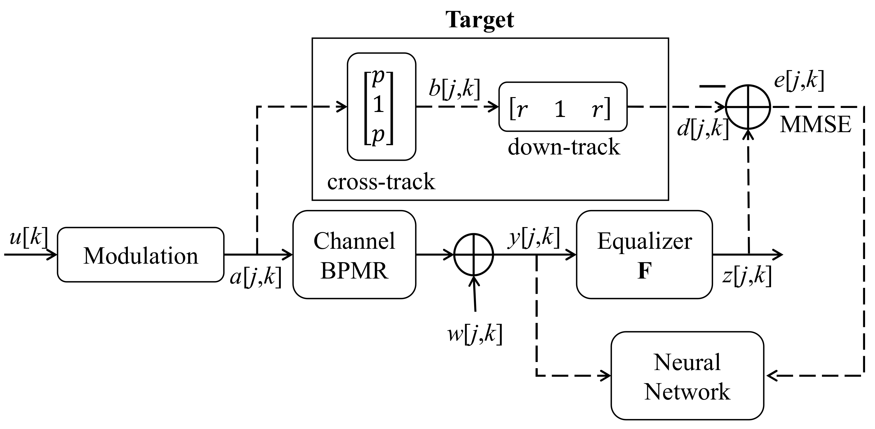
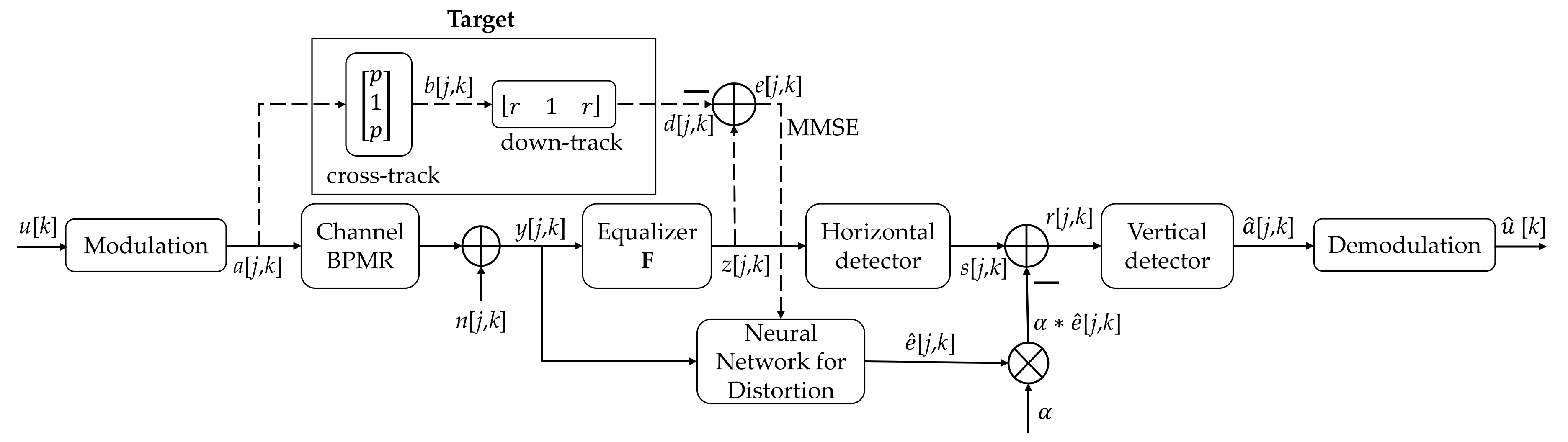
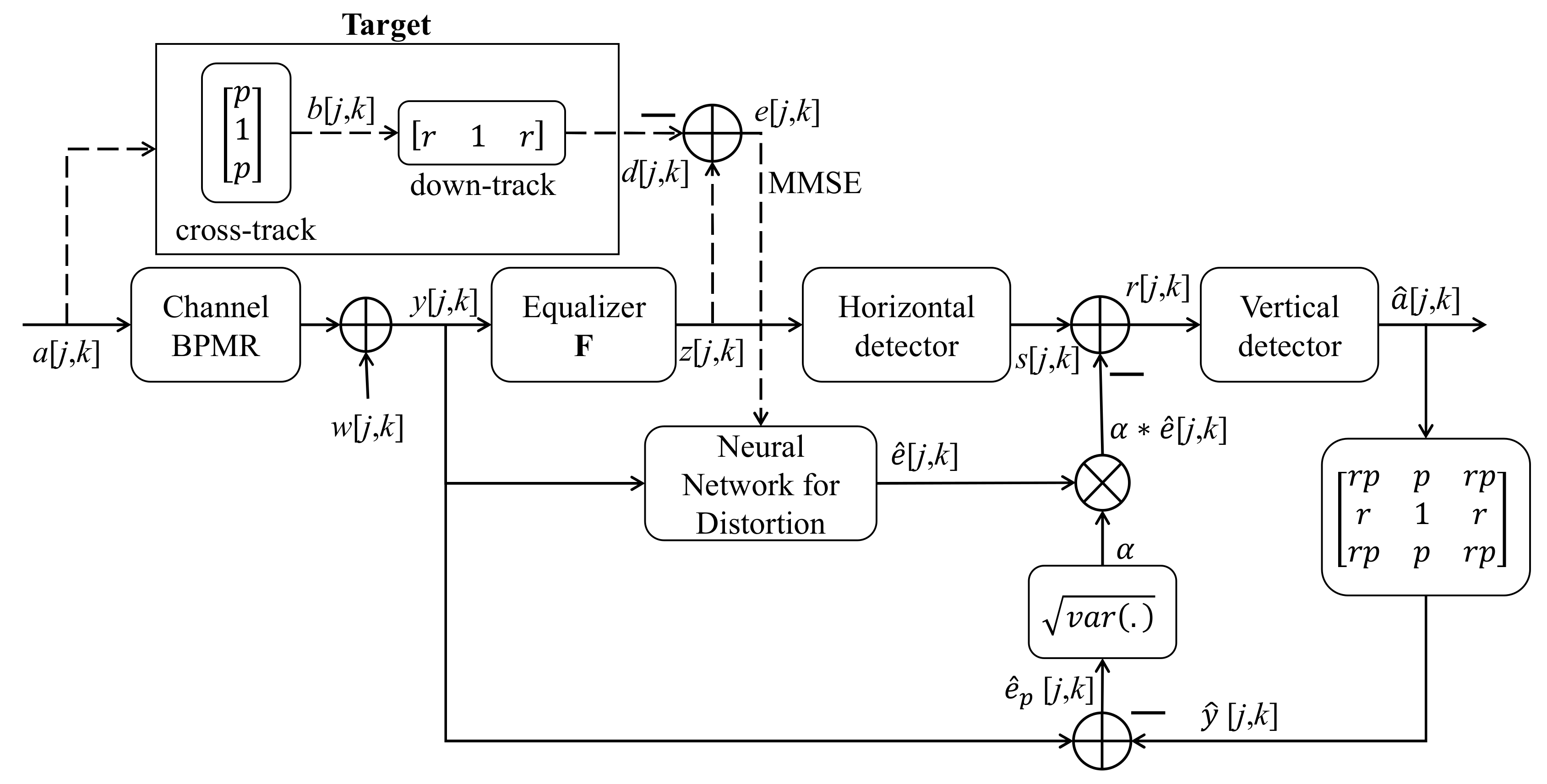
3. Proposed Model

The proposed model is illustrated in Figure 9 and comprises two processes (i.e., training and testing). In Figure 9, the dashed line is the stream of the signal in the training process, and the solid line is the stream of the signal in both the training and testing processes. In the training process, after target estimation, we achieved the error signal e[j,k], which was used to train the neural network. In this process, the neural network uses the signal y[j,k] as the input and the signal e[j,k] as the output (label). The signals s[j,k], r[j,k], $\widehat{a}$[j,k], and $\widehat{e}$[j,k] do not appear in the training process, as shown in Figure 5.

In the testing process, in Figure 9, the signal does not go through the path indicated by the dashed line but only through the one denoted by the solid line. The original data u[k] is magnetized (i.e., modulated) into the signal a[j,k] ∈ {−1,1}, and the data are stored in the BPMR channel. When the data are read back, the readback signal y[j,k] is affected by the additive noise, TMR, and media noise. The received signal is equalized by the equalizer F and converted into the desired signal d[j,k]. However, the readback signal y[j,k] that is converted to z[j,k] is not the same as the desired signal d[j,k]. 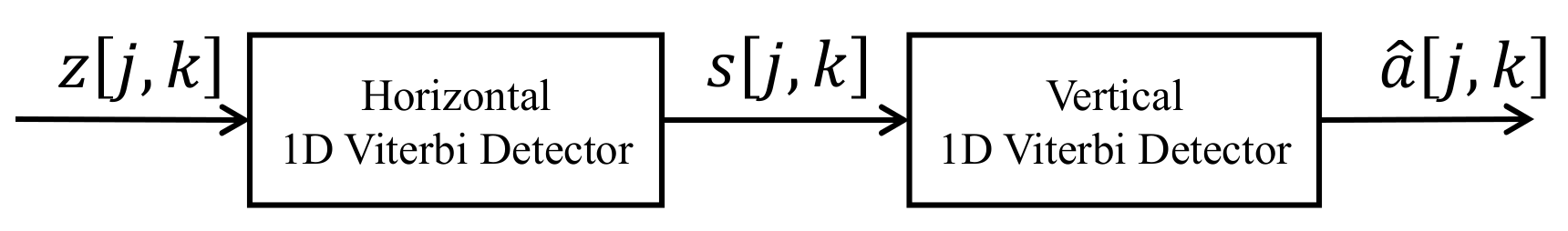The signal z[j,k] goes through the serial detection, which includes a horizontal detector (inner detector) and a vertical detector (outer detector). The neural network extracts the error signal $\widehat{e}$[j,k] from the received channel output signal y[j,k], and $\widehat{e}$[j,k] is slightly clearer between the desired signal d[j,k] and the received signal y[j,k]. The noise information $\widehat{e}$[j,k] from the neural network is supplied after the inner detection to create the soft output r[j,k] for the outer detector and improve the bit error rate (BER) performance of the systems. The serial detection output $\widehat{a}$[j,k] is demodulated to recover the original signal $\widehat{u}$[j,k].

3.1. BPMR Channel

In the system, the signal a[j,k] ∈ {−1,1} is stored in the BPMR channel by magnetizing the original data u[k] ∈ {0,1}. In the BPMR channel, the readback signal is distorted by the interference and additive white noise as follows:

$$y\left[j,k\right]=a\left[j,k\right]*c\left[j,k\right]+w\left[j,k\right],$$

(8)

where a[j,k], c[j,k], and w[j,k] are the 2D discrete input data, 2D channel response, and the electronic noise modeled as the additive white Gaussian noise (AWGN) with zero mean and variance ${\sigma }^2$, respectively.

The 2D channel response c[j,k] is presented in (9), which is a sampling of a 2D Gaussian pulse response in (10) and used to simulate the 2D island response [8,25,28].

$$c\left[j,k\right]=P\left(j{T}_x,k{T}_z\pm {\Delta }_{off}\right),$$

(9)

$$P\left(x,z\right)=A\exp \left(-\frac{1}{2q^2}\left[{\left(\frac{x+{\Delta }_x}{P{W}_x}\right)}^2+{\left(\frac{z+{\Delta }_z}{P{W}_z}\right)}^2\right]\right),$$

(10)

where x and z are the time indices in the down-track and cross-track directions, respectively. ${∆}_x$ and ${∆}_z$ are the bit location fluctuations, A is the peak amplitude of the 2D Gaussian function, q represents the relationship between the standard deviation of a Gaussian function and PW₅₀, which is the pulse width at half of the peak amplitude, and q is 1/2.3548; and PW_x and PW_z are the PW₅₀ components of the down-track and cross-track pulses, respectively; j and k represent the time indices of the isolated island in the cross-track and down-track directions, respectively. Additionally, we define the TMR for the BPMR system as

$$\mathrm{TMR}\left(\%\right)=\frac{{\Delta }_{off}}{T_z}.$$

(11)

3.2. Equalizer

To implement a 2D GPR equalizer, we need to use a buffer for processing each data page. In the training process, the parameters of the equalizer and GPR target are estimated by solving Equation (1). We define the equalizer and GPR target as matrices F and G, respectively.

$$\mathbf{F}=\left[\begin{array}{ccccc}{f}_{-2,-2}& f_{-2,-1}& f_{-2,0}& f_{-2,1}& f_{-2,2}\\ f_{-1,-2}& f_{-1,-1}& f_{-1,0}& f_{-1,1}& f_{-1,2}\\ f_{0,-2}& f_{0,-1}& f_{0,0}& f_{0,1}& f_{0,2}\\ f_{1,-2}& f_{1,-1}& f_{1,0}& f_{1,1}& f_{1,2}\\ f_{2,-2}& f_{2,-1}& f_{2,0}& f_{2,1}& f_{2,2}\end{array}\right],$$

(12)

$$\mathbf{G}=\left[\begin{array}{ccc}{g}_{-1,-1}& g_{-1,0}& g_{-1,1}\\ g_{0,-1}& g_{0,0}& g_{0,1}\\ g_{1,-1}& g_{1,0}& g_{1,1}\end{array}\right],$$

(13)

We convert the matrix F and matrix G into the vector f and vector g as below:

$$\mathbf{f}={\left[\begin{array}{ccccccc}{f}_{-2,-2}& f_{-2,-1}& \dots & 0& \dots & f_{2,1}& f_{2,2}\end{array}\right]}^T,$$

(14)

$$\mathbf{g}={\left[\begin{array}{ccccccc}{g}_{-1,-1}& g_{-1,0}& \dots & 0& \dots & g_{1,0}& g_{1,1}\end{array}\right]}^T,$$

(15)

From (14) and (15), the desired signal d[j,k] and the equalized signal z[j,k] can be expressed as follows:

$$d\left[j,k\right]=g^{T}a$$

(16)

$$z\left[j,k\right]=f^{T}y\mathrm{a}=1$$

(17)

where

$$a={\left[\begin{array}{cccccc}a[j+1,k+1]& a[j+1,k]& \dots & 0& \dots & a[j-1,k-1]\end{array}\right]}^T$$

(18)

$$y={\left[\begin{array}{cccccc}y[j+2,k+2]& y[j+2,k+1]& \dots & 0& \dots & y[j-2,k-2]\end{array}\right]}^T$$

(19)

The error signal e[j,k] is presented as follows:

$$e\left[j,k\right]=z\left[j,k\right]-d\left[j,k\right]={\mathbf{f}}^T\mathbf{y}-{\mathbf{g}}^T\mathbf{a}.$$

(20)

Then, the MSE can be expressed as follows:

$$\begin{array}{ll}E\left\{{\left(e\left[j,k\right]\right)}^2\right\}& =E\left\{\left({\mathbf{f}}^T\mathbf{y}-{\mathbf{g}}^T\mathbf{a}\right){\left({\mathbf{f}}^T\mathbf{y}-{\mathbf{g}}^T\mathbf{a}\right)}^T\right\}\\ & ={\mathbf{f}}^T\mathbf{Rf}-2{\mathbf{f}}^T\mathbf{Tg}+{\mathbf{g}}^T\mathbf{Ag}.\end{array}$$

(21)

where R is the autocorrelation matrix of the channel output data, R = E{yy^T}; T is the cross-correlation between the input data and the channel output data, T = E{ya^T}; and A is the autocorrelation of the input data, A = E{aa^T}, where E denotes the expectation, and T is the transpose operator.

In (1), the constraint can be expressed as follows:

$${\mathbf{E}}^T\mathbf{g}=\mathbf{b},$$

(22)

where

$$b={\left[\begin{array}{ccccc}0& 0& 1& 0& 0\end{array}\right]}^T,$$

(23)

and

$${\mathbf{E}}^T=\left[\begin{array}{ccccccccc}1& 0& 0& 0& 0& 0& 0& 0& 0\\ 0& 0& 1& 0& 0& 0& 0& 0& 0\\ 0& 0& 0& 0& 1& 0& 0& 0& 0\\ 0& 0& 0& 0& 0& 0& 1& 0& 0\\ 0& 0& 0& 0& 0& 0& 0& 0& 1\end{array}\right].$$

(24)

Based on these constraints, we derive the Lagrange multiplier, optimal target, and equalizer coefficient vectors as follows [18]:

$$\lambda ={\left(E^T{\left(A-T^T{R}^{-1}T\right)}^{-1}E\right)}^{-1}b,$$

(25)

$$g={\left(A-T^T{R}^{-1}T\right)}^{-1}E\lambda ,$$

(26)

$$g_{-1,1}=g_{1,-1}=g_{1,1}=g_{-1,-1}=g_{-1,0}.g_{1,-1},$$

(27)

$$f=R^{-1}Tg,$$

(28)

Equation (27) is a constraint that ensures the form of matrix G in [18]. These parameters are used in the testing process.

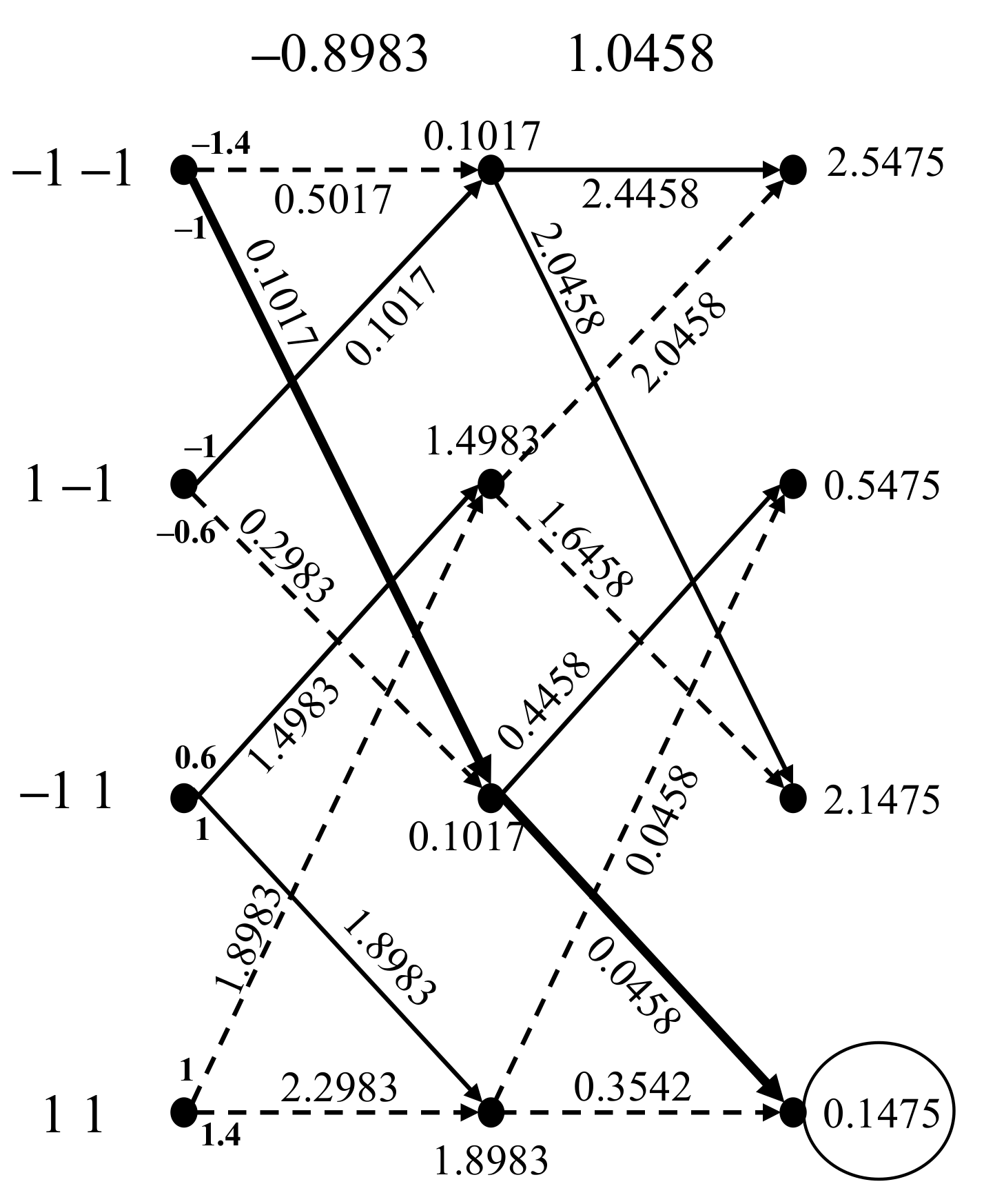
3.3. Serial Detection with Noise Prediction

To implement the serial detection, we also need a buffer to get the j×k data because the horizontal and vertical detectors process the 2D data in different directions. The output of the equalizer z[j,k] is fed into the horizontal detector (inner detector). When the VA is applied with the horizontal interference coefficients, the output signal s[j,k] of the inner detector has six levels. Consequently, s[j,k] − $\widehat{e}$[j,k] is used to obtain the soft output signal r[j,k], where the signal $\widehat{e}$[j,k] is the predicted signal of the signal e[j,k] in the testing process. Finally, the signal r[j,k] goes to the vertical detector and restores the signal $\widehat{a}$[j,k].

In [19], the authors used a feedback line to reduce the down-track interference and added the remaining cross-track interference to the hard output of the inner detector to create the soft output signal s[j,k]. This preserves the noise information to be correct in the next detector. However, this does not achieve the full characteristics of the nonlinear interference. Therefore, in this study, we used a neural network to predict the noise signal, because predicting the noise signal from the received signal is a nonlinear problem, and the neural network is therefore more appropriate than a linear equalizer.

4. Simulation and Results

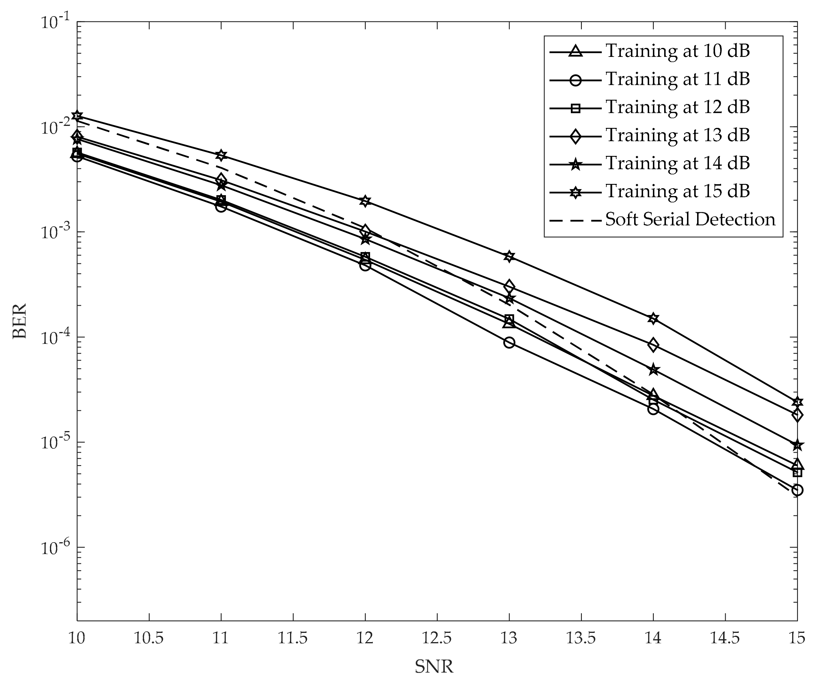
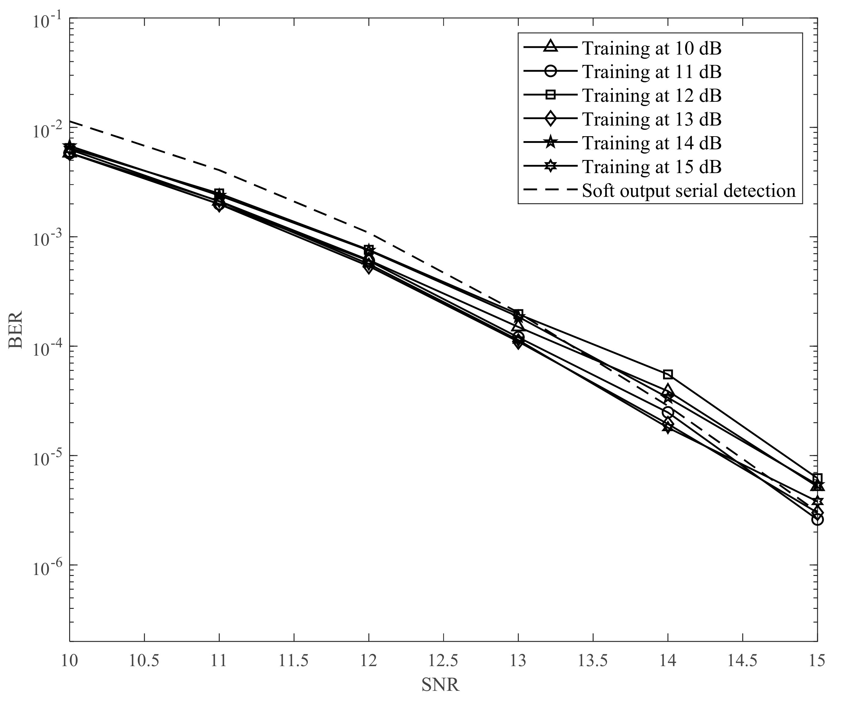
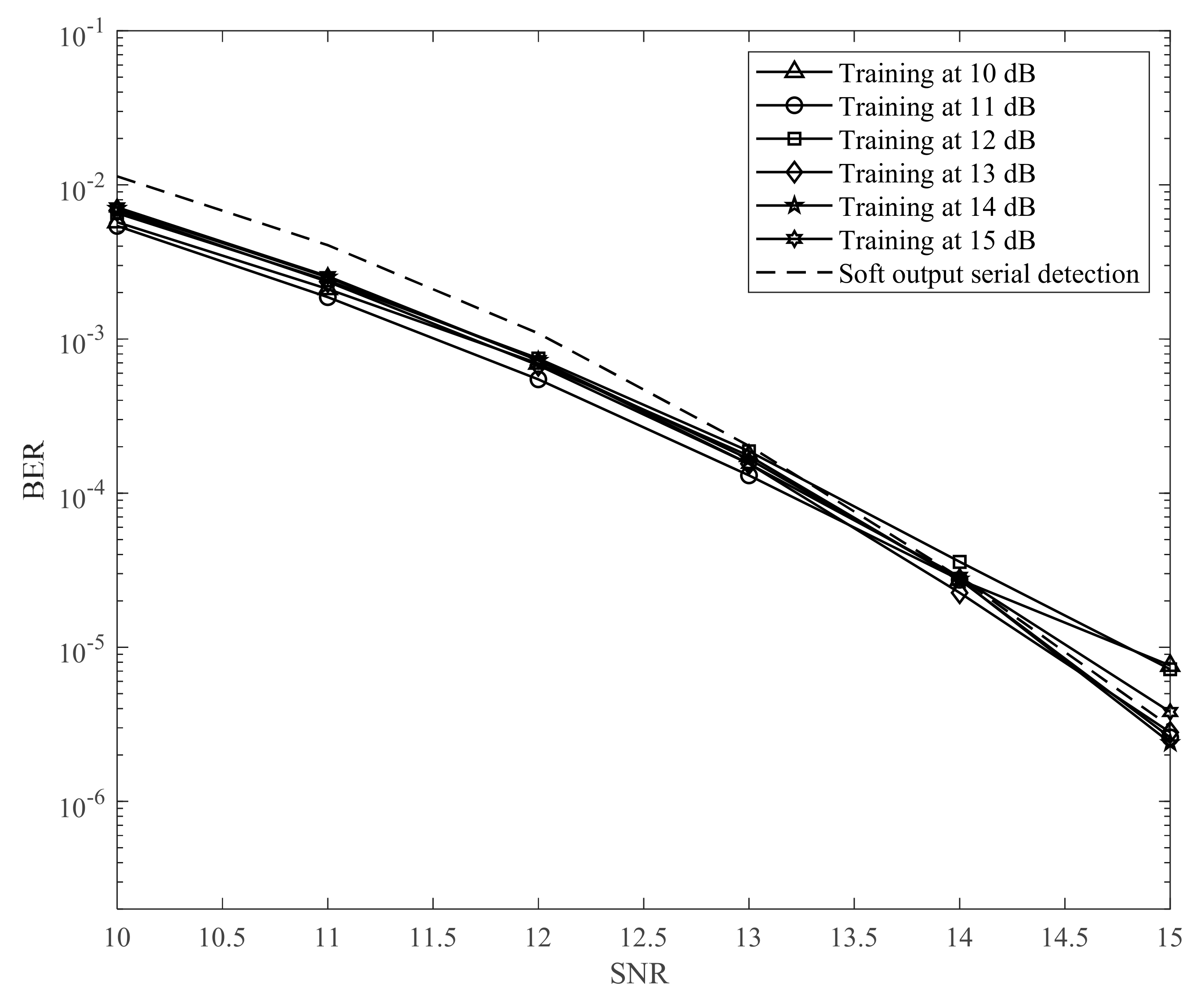
We performed the simulation using MATLAB 2019 and set up the environment as detailed in this section. In the training process, we used the model shown in Figure 5. We applied the MMSE algorithm to find the parameters in the equalizer and GPR target, as in Section 3.2. Thereafter, we created 3000 random samples u[k] ∈ {0,1} with a length of 10,000 and reshaped the signal a[j,k] ∈ {−1,1} with a size of 100 × 100. In this study, we focus on combating ITI and ISI. Accordingly, we use the small block size of 100 × 100 data for 2D interference. The channel output y[j,k] is supplied to the input of the neural network, and the error signal e[j,k] is supplied to the output of the neural network as a label. Therefore, the neural network was trained with 3000 random samples. In the testing process, we created 1000 random samples u[k] with a length of 10,000 and reshaped the signal a[j,k] with a size of 100 × 100. The signal a[j,k] is fed into the channel to suffer 2D interference and additive noise. The channel output y[j,k] is converted into an equalized signal, z[j,k]. Further, the signal z[j,k] goes through serial detection, which utilizes our proposed method for creating the soft output, to detect and recover the modulated signal $\widehat{a}$[j,k]. Finally, $\widehat{a}$[j,k] is demodulated into the original signal $\widehat{u}$[k]. In this paper, we define the channel signal-to-noise ratio (SNR) as 10log₁₀(1/${\sigma }^2$), where ${\sigma }^2$ is the AWGN power. As shown in Figure 10, Figure 11 and Figure 12, we changed the SNR from 10 to 15 dB to train the neural network in the training process. Thereafter, in the testing process, we used the neural network models from 10 to 15 dB to simulate the BER performance. 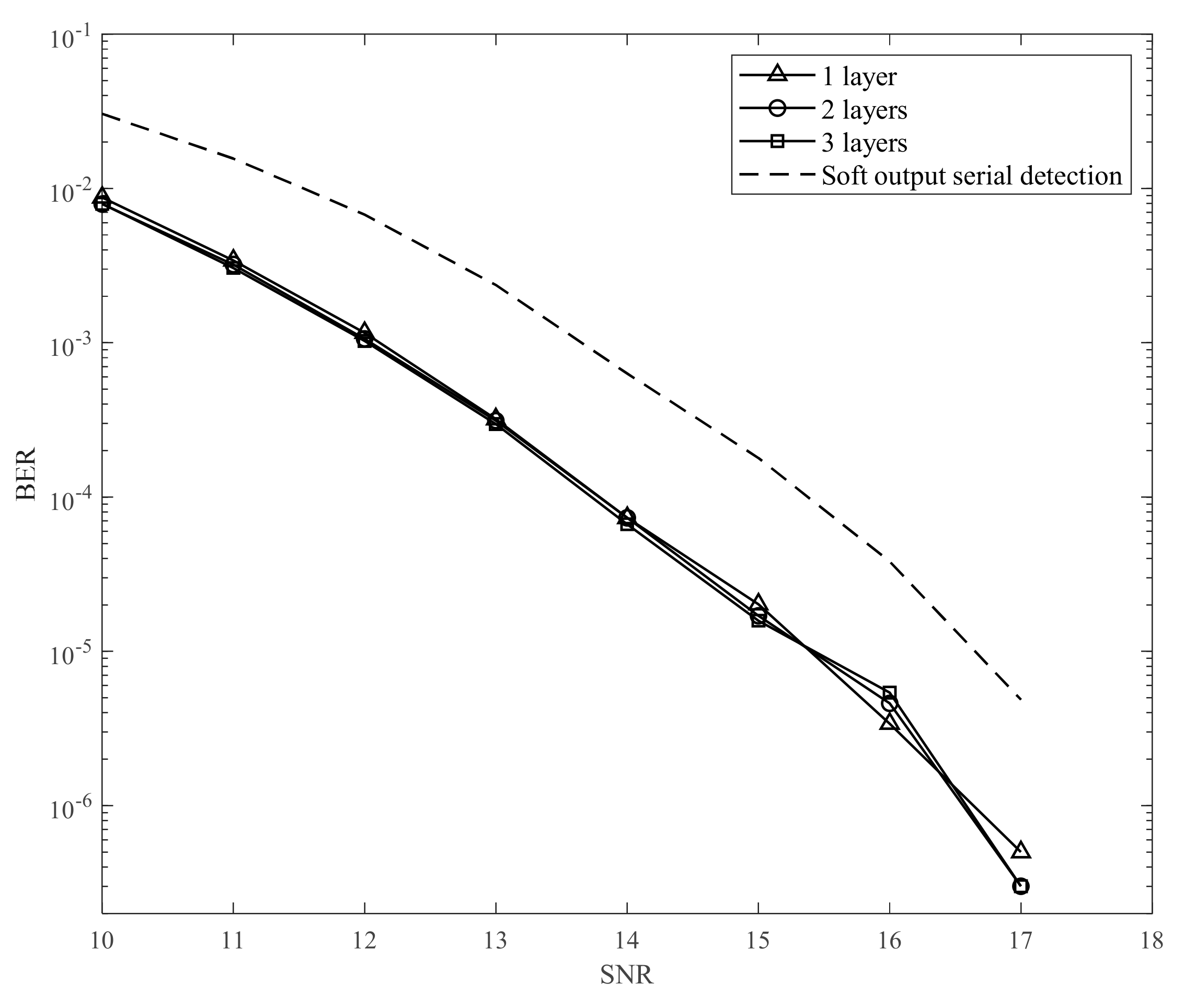In addition, Figure 10, Figure 11 and Figure 12 have hidden layers [100] (one layer), [60 40] (two layers), and [30 50 20] (three layers), respectively. We simulated an AD of 3 Tb/in² (0.465 Tb/cm²) (T_x = T_z = 14.5 nm) [18,19]. The coefficient of the channel, which does not include the TMR effect (${∆}_{off}=0$) or media noise (${∆}_x={∆}_z=0$), was used in the simulation as follows:

$$H=\left[\begin{array}{ccc}0.0824& 0.3876& 0.0824\\ 0.2125& 1& 0.2125\\ 0.0824& 0.3876& 0.0824\end{array}\right].$$

(29)

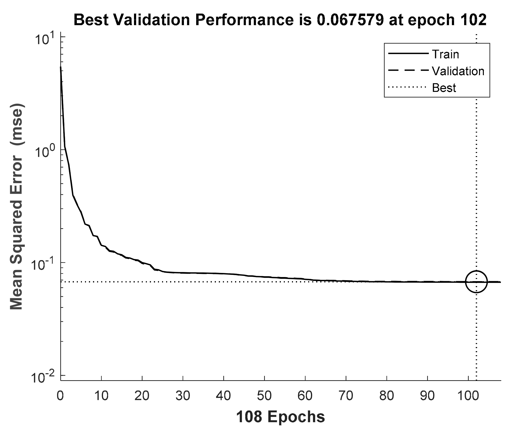
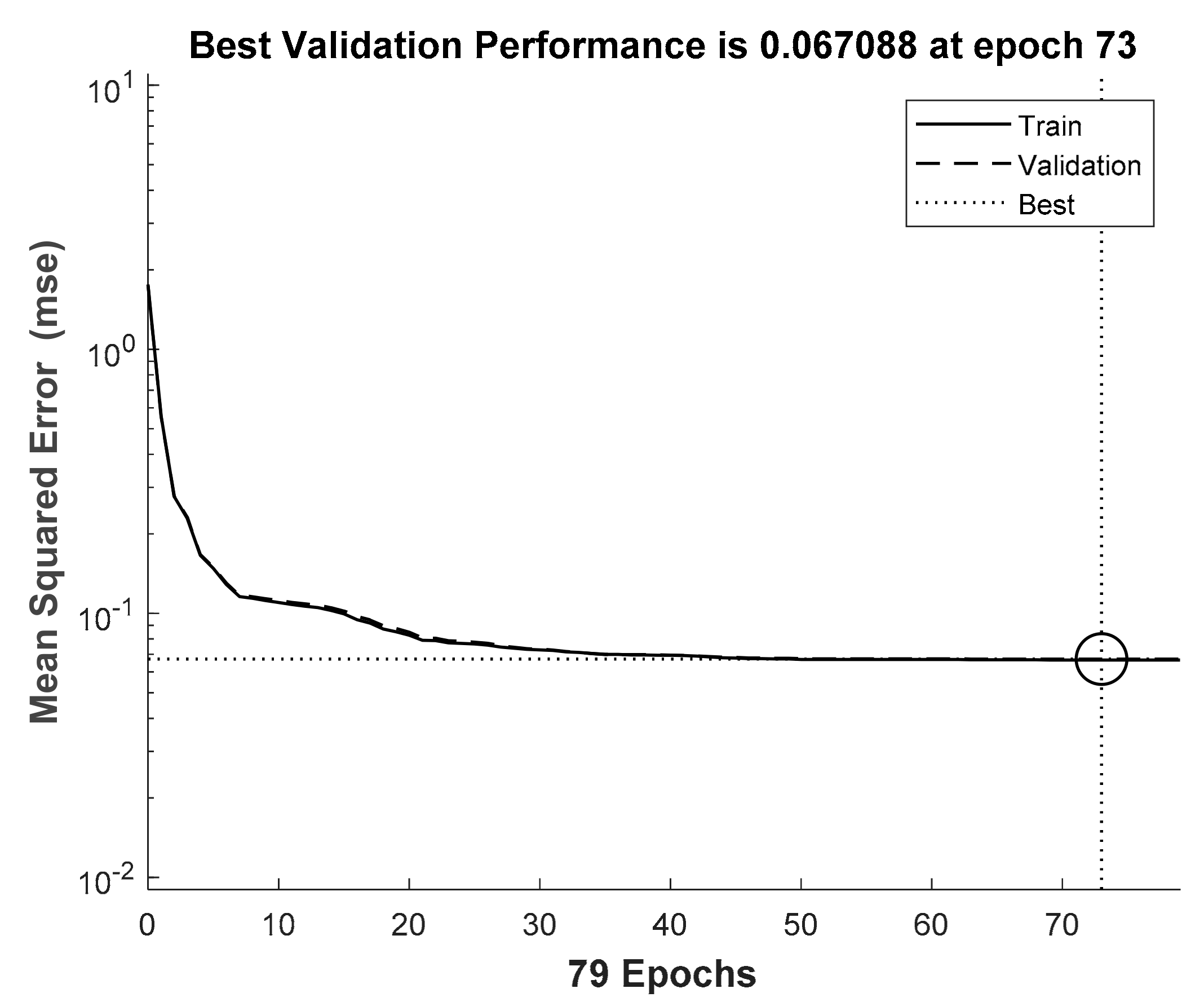
4.1. Second Proposed Model

The results in Figure 10, Figure 11 and Figure 12 indicate that the proposed model with the neural network can improve the BER performance only when the SNR is lower. To explain this issue, we considered the learning ability of the neural network. In the training process, if we train the neural network at a low SNR, the neural network is not suitable for predicting the noise at a higher SNR. Meanwhile, if we train the neural network at a high SNR, the signal e[j,k] is small. Consequently, the label in the training process is close to zero. Therefore, the neural network is overfitting to almost zero noise and cannot predict the noise when the SNR is large. To solve this problem, we propose the second model shown in Figure 13.

In Figure 13, the neural network is trained only at a constant SNR value to avoid the error signal e[j,k] being too small. We multiply a parameter $\alpha$ to compensate for the noise power at other SNR values in the testing process. Although the parameter is unknown, we need it to reduce the noise to increase the SNR. Therefore, the optimal value $\alpha$ is determined at each SNR value ranging from 0 to 1 in the testing process. Based on the results in Figure 10, Figure 11 and Figure 12, we chose the best case, which is the neural network trained at 11 dB. The noise e[j,k] is not too small, and thus, it achieves the gain. 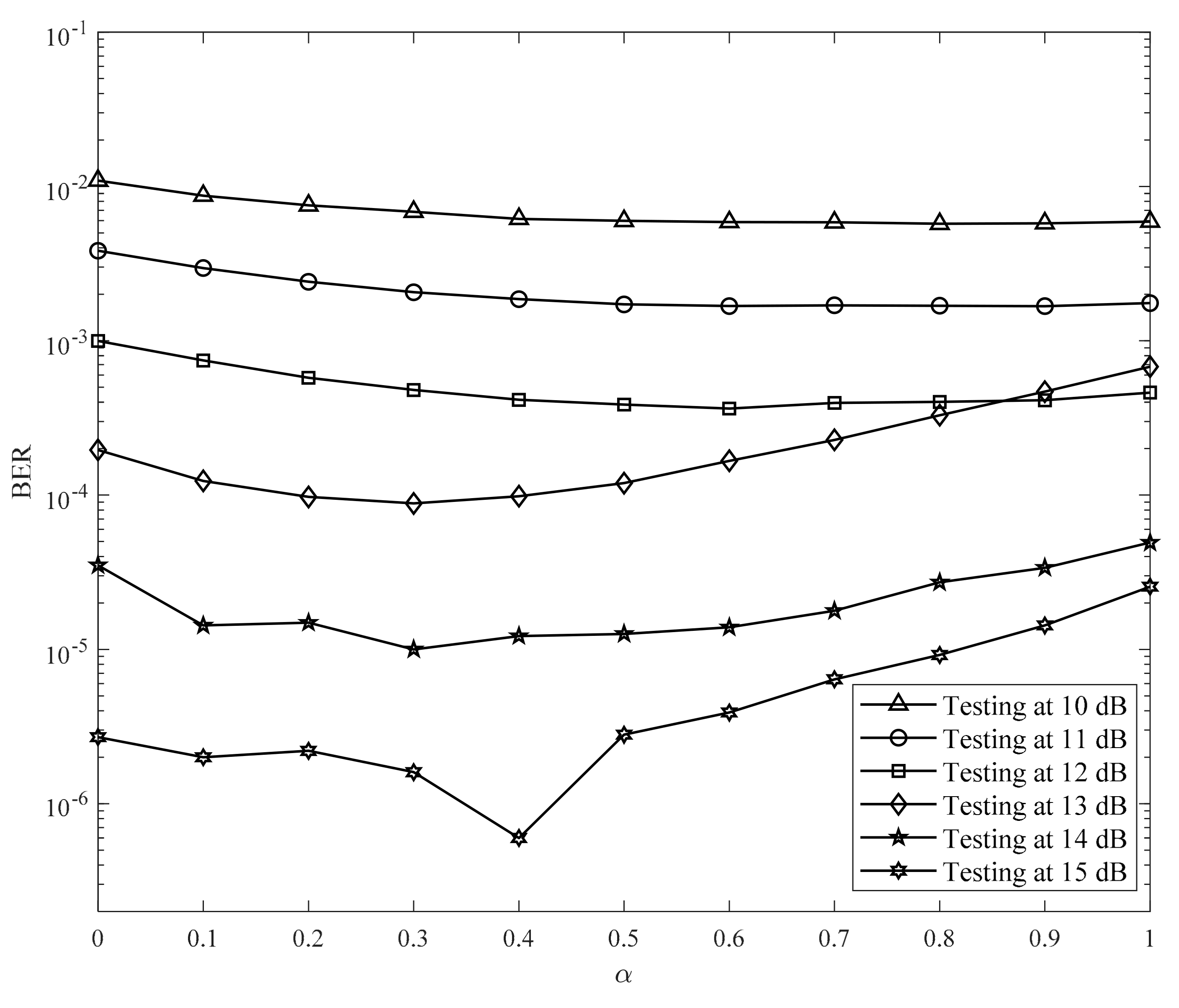In Figure 14, we used the two hidden layer neural networks trained at 11 dB while changing the parameter $\alpha$ from 0 to 1 with step size of 0.1, and tested it from 10 to 15 dB. The optimal values of $\alpha$ for each SNR are listed in

Table 6. The optimal value $\alpha$ corresponding to SNR.

SNR	10 dB	11 dB	12 dB	13 dB	14 dB	15 dB
α	0.8	0.9	0.6	0.3	0.3	0.4

; the values of $\alpha$ decrease as the SNR increases. As the noise power must be decreased for a high SNR, the optimal values of $\alpha$ also decrease.

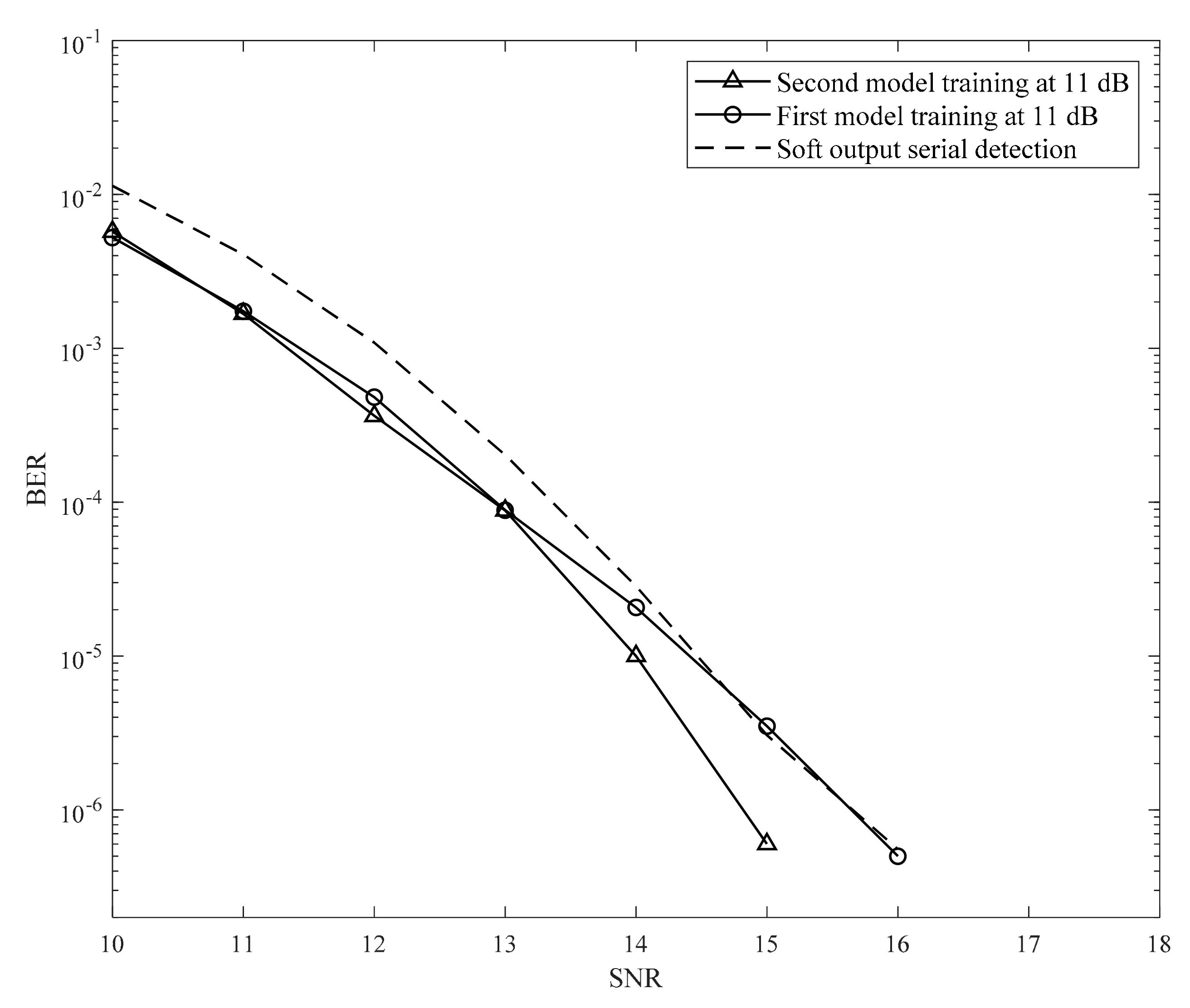
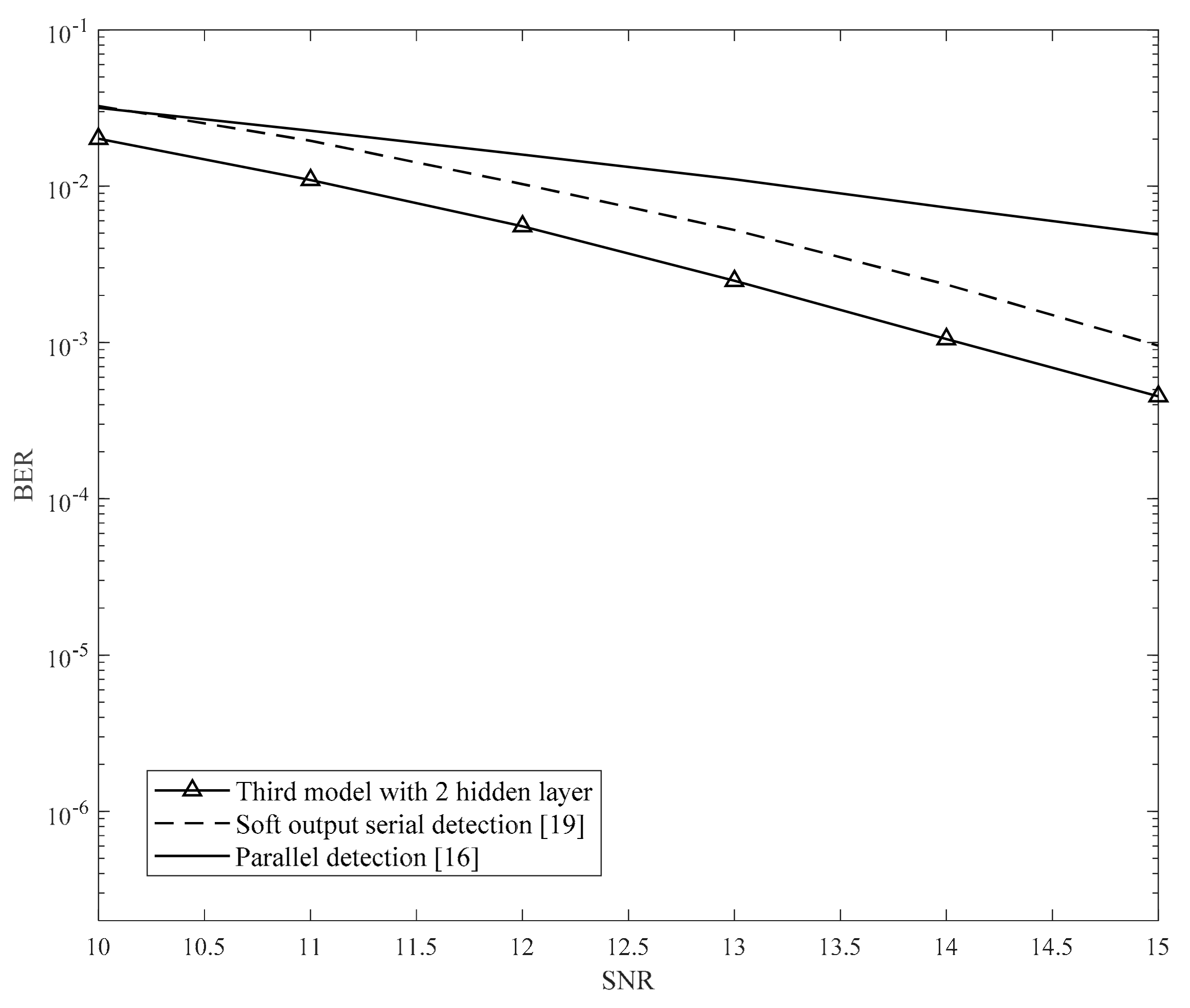
By applying the optimal parameter $\alpha$, we achieve the BER performance of the second proposed model with two hidden layers, as shown in Figure 15. The results indicate that the second model achieves a gain of 1 dB at a BER of 10⁻⁶ compared to the serial detection in [19]. In addition, this method was easier to implement.

4.2. Third Proposed Model

With the second model, we can achieve the desired results in theory. However, given the survey to determine the optimal parameter $\alpha$, it is cumbersome. Therefore, we propose the third model, illustrated in Figure 16.

This model uses the feedback from the signal $\widehat{a}$[j,k] to estimate the interfered signal $\widehat{y}$[j,k] without any random noise. We know that the received signal y[j,k] includes the 2D interfered signal $\widehat{y}$[j,k] along with noise. Therefore, the received signal is subtracted by $\widehat{y}$[j,k] to obtain the noise signal $\widehat{e}$_p[j,k]. Then, the parameter $\alpha$ is given by the square root of the variance of the noise signal $\widehat{e}$_p[j,k] and multiplied by the signal $\widehat{e}$[j,k]. The results of the third model are shown in Figure 17.

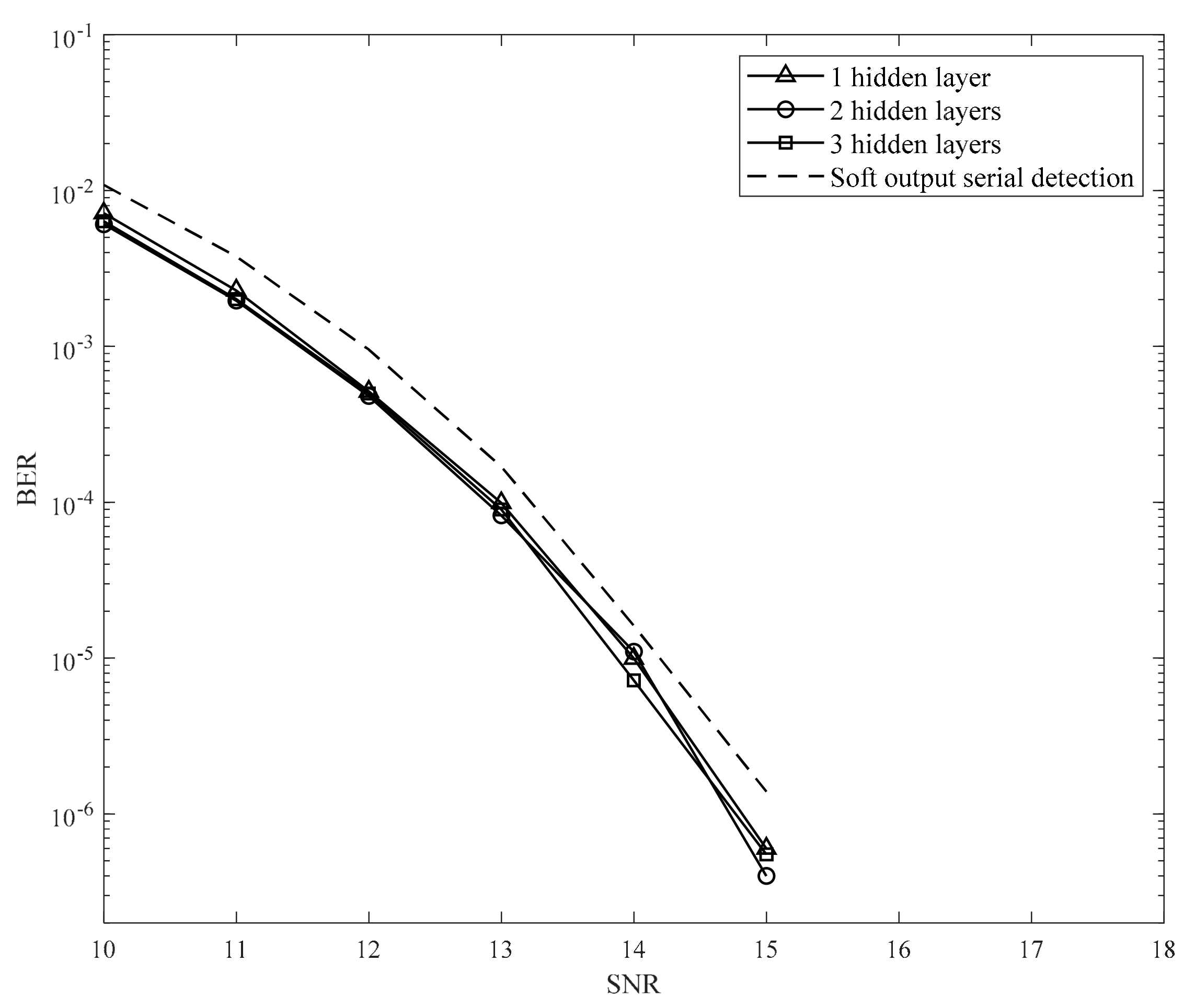
For the third model, we trained the neural network at an SNR of 11 dB and used one to three hidden layers. To clarify the effectiveness of deep learning, we increase the training data. We use 5,000 random samples to train for this model. Although the complexity of the third model is higher than that of the second model, we do not need to conduct a survey to determine the optimal value of $\alpha$ and do not spend considerable time on the training process. Moreover, this model achieves a performance similar to the second model.

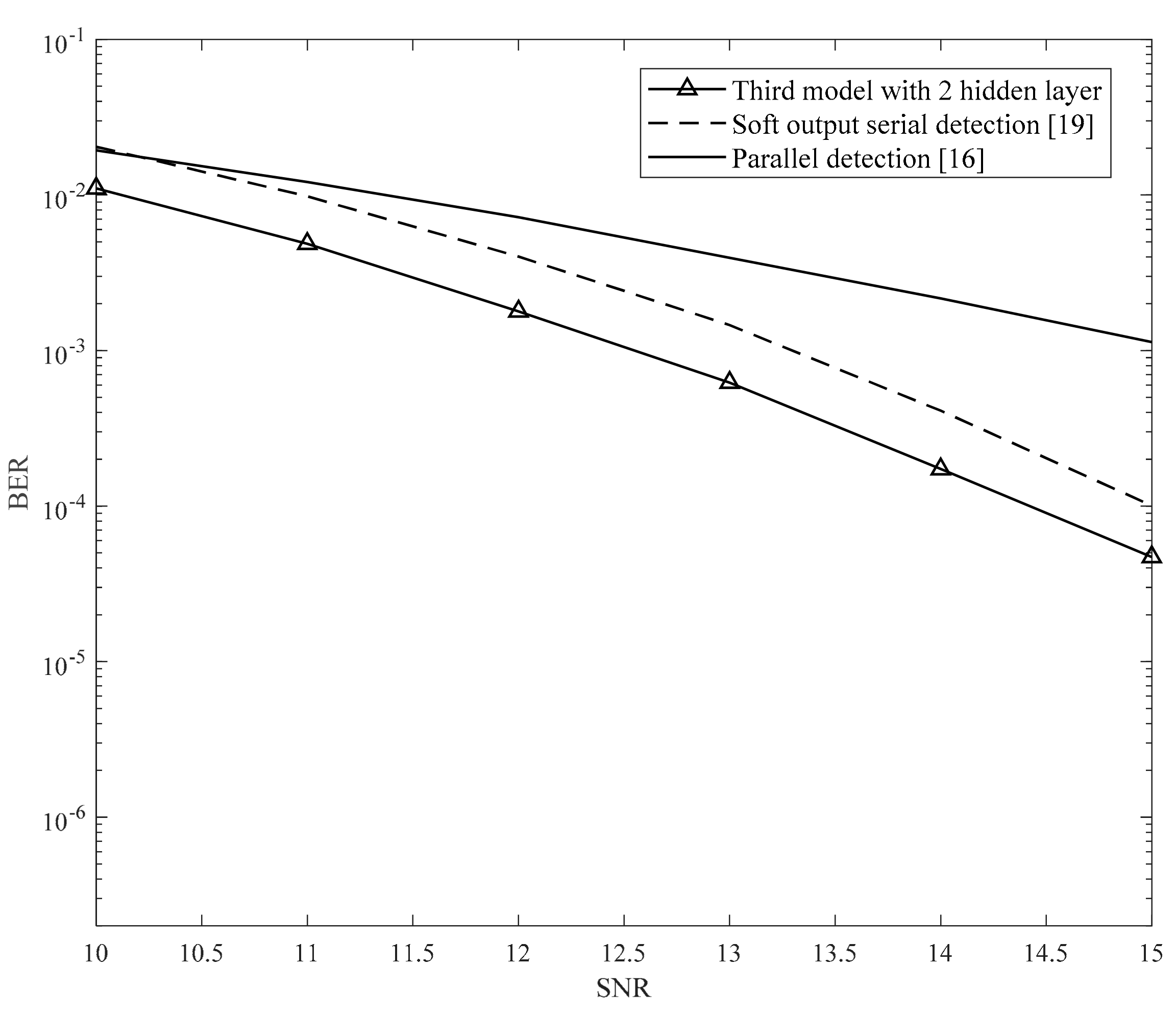
We also compared our proposed method with the BCJR algorithm, which is represented by the IRCSDF-GA algorithm in [21]. In [21], the authors also showed that the results in [20,21] were similar; however, for simplicity, we implemented the algorithm in [21]. In theory, the MAP algorithm achieves a better performance than the ML algorithm. However, in [20,21], the MAP algorithm is not suitable for 2D interference; therefore, it cannot achieve the theoretical results. For complexity, the IRCSDF-GA’s trellis includes four states with two input branches in each state. The IRCSDF-GA algorithm has two trellises for rows and columns, respectively. In each trellis, the computation consists of determining the branch, forward, and backward metrics. Therefore, it is evident that the IRCSDF-GA is more complicated than the serial detection model. In the serial detection model, the inner detection trellis included four states and six input branches, and the outer detection trellis included four states and two input branches. Both the inner and outer detections’ computations need only to find the branch metric.

Furthermore, the ITI and ISI are equal in [20], whereas ITI is more severe than ISI in this study. Therefore, there is a gain difference between this study and [20]. In addition, in [20,21], the authors designed the IRCSDF algorithm with a known channel parameter, and this is not appropriate for a real situation where we cannot explicitly identify the channel.

In addition, we also compare our proposal with the ConvNet detector in [29]. However, the ConvNet detector cannot achieve high performance, because the ConvNet detector is designed for collaborating with the low-density parity code (LDPC). Therefore, the ConvNet detector achieves low BER performance when we use it alone.

From the results of the second and third models, we can see that the parameter $\alpha$ helps the neural network adapt to the environment when the SNR is high. Also, the performance is almost the same even if the number of hidden layers is changed.

4.3. Proposed Model with TMR Effect

In BPMR systems, the TMR effect significantly degrades the BER performance. Usually, in practice, we do not know how much TMR affects the system. Therefore, in this simulation, we assume that the system suffered 10% TMR and 20% TMR in Figures 19 and 20, respectively. In this experiment, we just used the third model to consider the system’s resistance to the TMR effect. In addition, we used the BPMR channel with the parameter $-{∆}_{off}$ in Section 3.1 to create the TMR effect.

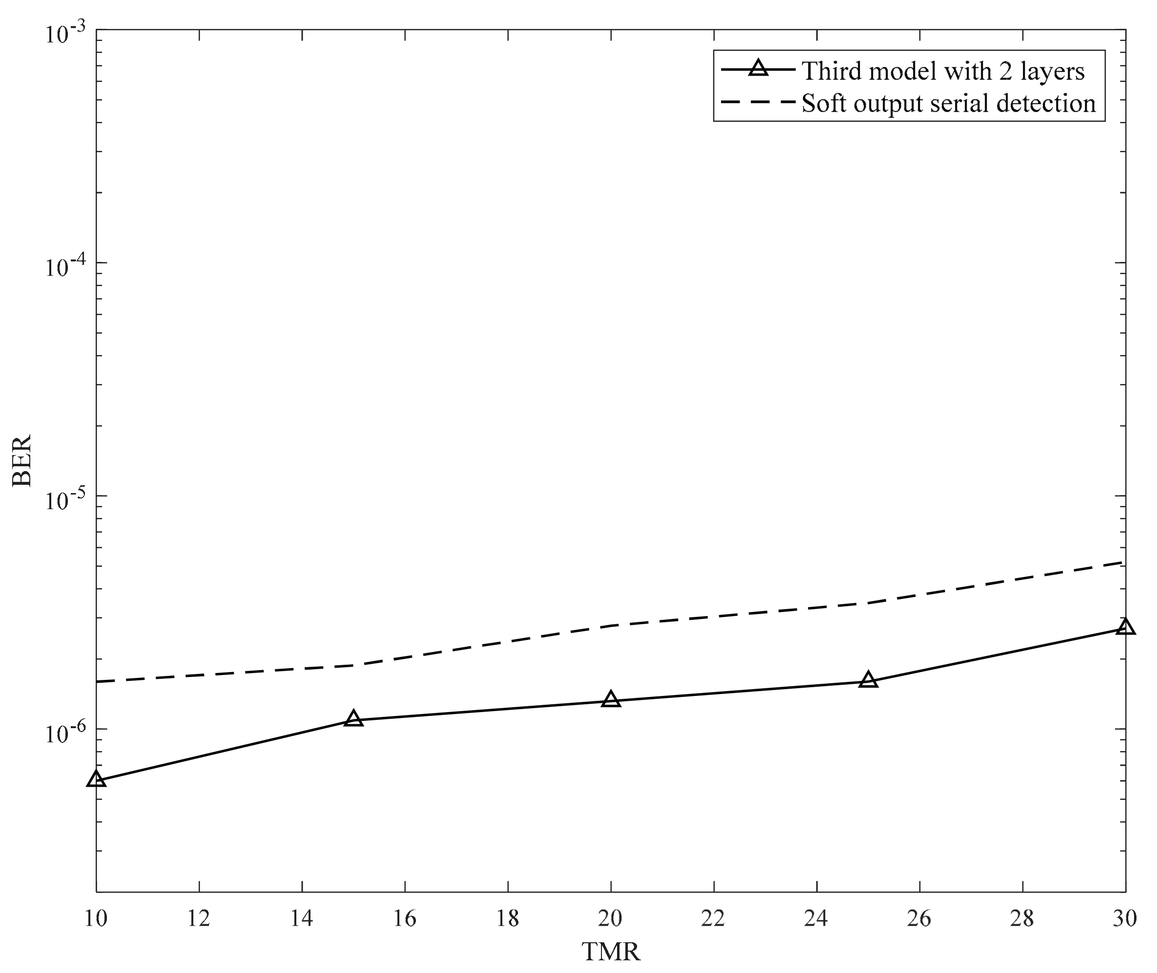
Figure 19 illustrates the BER performance when the TMR was varied from 10% to 30% at SNR of 15 dB. Consequently, the system primarily suffers from the TMR effect rather than by additive noise. The neural network was trained at SNR of 11 dB and had two hidden layers.

As shown in Figure 18 and Figure 19, the proposed model performs better than the serial detection in [19]. In Figure 19, the proposed model is shown to exhibit the ability to overcome the TMR effect.

4.4. Our Proposed Model with Media Noise

To approximate the actual condition, we simulated the BPMR system with position fluctuation. Based on the BPMR channel in Section 3.1, in Figure 20, we performed a simulation with 6% position fluctuation (${∆}_x\ne 0$ and ${∆}_z\ne 0$) [19]. In addition, we simulated the third model with position fluctuation. The neural network was trained at an SNR of 11 dB.

In Figure 20, at 6% position fluctuation [30], the proposed model significantly improves the BER performance compared to the serial detection in [19]. This depicts the predicting ability of the neural network. When the neural network is trained in the position fluctuation condition, it can also predict the level of position fluctuation. To further investigate the position fluctuation, we fixed the SNR at 15 dB and changed the position fluctuation from 6% to 18%. 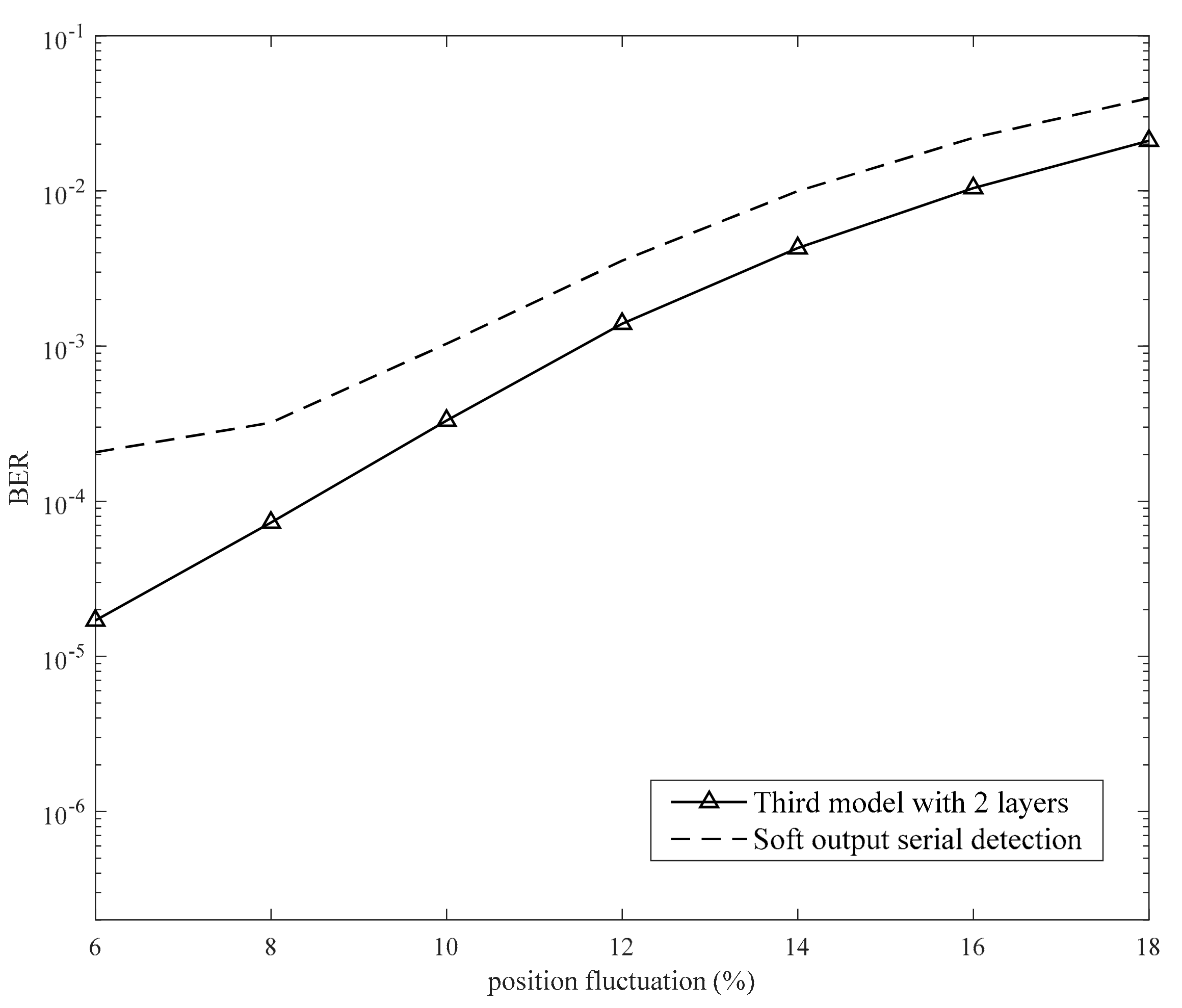The results are presented in Figure 21 and indicate that the proposed model can resist a position fluctuation of less than 18%. If the position fluctuation is more than 18%, the proposed model cannot achieve the gain.

In addition, Figure 22 and Figure 23 illustrate the experiment results on the channel with (10% TMR, 6% position fluctuation) and (15% TMR, 8% position fluctuation), respectively. The results show that our proposed model still achieves the gain compared with the previous studies when suffering both TMR and media noise effect.

Finally,

Table 7. The complexity for our proposed and other methods.

Method	Mul/div	Add/sub	Exp/log	Sqrt
Our model	4291	4839	100	1
1 DNN [31]	12953	11087	18	16
8 DNN [31]	101013	86528	18	16
LAIP-BCJR [32]	291560	189279	257	0
CNN [32]	113761	102062	1	0

compares the complexity among the proposed model and some previous studies [31,32] that applied the neural network for the TDMR channel. We use the third model with two hidden layers for comparison. We can see that the proposed model achieves manageable complexity.

5. Conclusions

In this study, we developed a method to improve the serial detection. All three models proposed use noise information to create the soft output for the inner detector in serial detection. However, the second and third models estimate noise information more precisely than the first model. The results showed that the second and third models significantly improved the BER performance. The proposed method also shows that it is less complex than the IRCSDF-GA algorithm. Instead of using the MAP algorithm to create the soft output, our model used the ML algorithm and added the noise information to create a soft output. In addition, the proposed model not only removes the 2D interference but also resists the effect of TMR and position fluctuation, because the neural network can learn and adapt to TMR effects and media noise, which have nonlinear characteristics.

Finally, in the ideal case, our proposed model can achieve an approximately 1 dB gain at 10⁻⁶ dB, which is evidently superior to the previously reported serial detection method.