Review

Independent Component Analysis Applied on Pulsed Thermographic Data for Carbon Fiber Reinforced Plastic Inspection: A Comparative Study

by
Julien R. Fleuret
*,†,
Samira Ebrahimi
,
Clemente Ibarra-Castanedo
and
Xavier P. V. Maldague
Computer Vision and Systems Laboratory (CVSL), Department of Electrical and Computer Engineering, Faculty of Science and Engineering, Laval University, Quebec City, QC G1V 0A6, Canada
*
Author to whom correspondence should be addressed.
These authors contributed equally to this work.
Appl. Sci. 2021, 11(10), 4377; https://doi.org/10.3390/app11104377
Submission received: 11 March 2021 / Revised: 21 April 2021 / Accepted: 7 May 2021 / Published: 12 May 2021
(This article belongs to the Special Issue Structural Health Monitoring & Nondestructive Testing)

Abstract

:
Dimensional reduction methods have significantly improved the simplification of Pulsed Thermography (PT) data while improving the accuracy of the results. Such approaches reduce the quantity of data to analyze and improve the contrast of the main defects in the samples contributed to their popularity. Many works have been proposed in the literature mainly based on improving the Principal Component Thermography (PCT). Recently the Independent Component Analysis (ICA) has been a topic of attention. Many different approaches have been proposed in the literature to solve the ICA. In this paper, we investigated several recent ICA methods and evaluated their influence on PT data compared with the state-of-the-art methods. We conducted our evaluation on reference CFRP samples with known defects. We found that ICA outperform PCT for small and deep defects. For other defects ICA results are often not far from the results obtained by PCT. However, the frequency of acquisition and the ICA methods have a great influence on the results.

1. Introduction

Non-Destructive Testing (NDT) is a very popular application in many fields of industry. Among the many different NDT domains, InfraRed Thermography (IRT) has become common for evaluating materials. IRT’s approaches consist in a set of tomographic approaches that are helpful to assess a wide range of features, from material homogeneity to the presence of void or foreign materials within another material. Within the field of IR-NDT, Pulsed Thermography (PT) is a well-known method. Among its fame are its simplicity and ability to provide valuable results on a wide range of materials [1,2]. During the PT experiment, a thermal camera is used in order to record the temperature decay. Thermal cameras are sensitive to a wide range of phenomenon and noises, including some created by themselves, resulting in a wide range of distortions during the creation of the data [3,4,5,6,7]. Therefore over time, many methods have been introduced in the literature. Pulsed Phase Thermography (PPT) [8] and Principal Component Thermography (PCT) [9] are among the most applicable. PPT consists in transforming the sequence into the Fourier domain and analyze the phase and PCT based on applying a PCA to the sequence to extract the most meaningful frames. Since then many methods of dimensional reduction have been successfully used on PT data. The high efficiency and simplicity of such method has made them very popular. Recently a new approach has been investigated, the Independent Component Analysis (ICA). Initially, the mathematical foundations were laid in the 1980s [10] to solve Blind Signal Separation (BSS). For BSS application on PT data is assumed that the data are the mixing of the uneven heating, the signal corresponding to the defective regions, the signal corresponding to the non-defective regions, and other noises and stochastic information that can be recorded. Solving the objective function of the ICA can be done by using several methods, and therefore performing an ICA is still the topic of intensive researches. ICA was also the topic of several recent works in IRT [11,12,13,14,15]. For these reasons, we wish to investigate how different approaches regarding the ICA computation can affect the defect detection in Carbon Fiber Reinforced Plastic (CFRP). The CFRP is used in a larger number of studies due to its physical properties, making sub-surface defects easier to detect. We limited our study to unsupervised ICA methods. The reason for this choice regards the difficulty to have a large number of labelled samples in order for a supervised algorithm to fit the data properly. Also, supervised approaches often require more work regarding preparing the data and more complex training and testing before for us to evaluate them.
The first contribution of this paper is to provide an extensive literature review of the most recent works involving CFRP and PT data. We investigated a quantitatively different method to compute the ICA. Finally, we investigated how the number of component in dimensionality reduction algorithms can affect the results, both quantitatively and qualitatively.

2. Literature Review

As previously mentioned, the sensibility of a thermal camera to noises makes the field of PT eager for new processing methods. In this section, we briefly introduce some of the most recent work. Inspired by the work of Maldague et al., known as PPT, Fleuret et al., investigated a feature base approach based on monogenic signal reconstruction for defect detection. Although the approach happened to be highly sensitive to noise, promising results were found. More recently, Netzelmann et al. [16] proposed two reformulations of the PPT, which improve the Contrast-to-Noise Ratio (CNR). Vavilov et al. [17] proposed a phase and time-domain tomography for defecting defects in composite materials. Poelman et al. [18] introduced an adaptive spectral processing. The method is more robust than the PPT, offers a better SNR even for barely visible defects. It also returns a single index map of the defects for a given sequence which makes it easier to interpret.
Another popular trend regarding the methods used to process PT data is the application of linear-algebra methods. Ahmed et al. [13] introduced an approach that consists of associating a sparse matrix factorization with a Mixture of Gaussian (MoG). The enhancement of the data is based on the sparse matrix factorization, which is solved as a minimization problem, in which the noise of the data is modeled by an MoG. The authors chose to model the noise in the data as an MoG due to its better reliability to the real case than traditional approaches that assume that the noise follows one model such as Gaussian or Laplacian. Later, the same authors introduced a wavelet-based approach in order to enhance the defect present in an image [19]. The same year they use this approach with a minimization approach, allowing them to separate a low-rank matrix, a sparse matrix, and a noise matrix from the data. They showed that this approach is state-of-the-art approaches [20]. Recently Ahmed et al. introduced another sparse low-rank optimization approach [21]. In this work, Ahmed et al. reuse the three matrix decomposition they already used in [20], but this time they introduced an activation function based on the immediate past in the cost function. Inspired by the work of Ahmed et al., Liu et al. [22] proposed an alternating sparse matrix decomposition. Like in the work of Ahmed et al., Liu et al., assumed that the data are the summation of three matrices, respectively a low-rank, a sparse, and the noise. They extend previous works by assuming that the sparse matrix is the product of a dictionary matrix with a matrix of weights. The goal of this assumption regarding the sparse matrix is to better model the background noises. Yousefi et al. [23] introduced the Candid-Covariance Free Principal Component Thermography (CCIPCT). CCIPCT is based on the work of Weng et al. [24] who has introduced the Candid-Covariance Free Principal Component Analysis (CCIPCA).
Wu et al. [25] introduced the SPCT, an application of the Sparse-PCA to PT. They showed that SPCT outperformed existing methods at a noticeably higher computational cost. The Sparse-PCA is a formulation of the PCA as a penalized regression problem under constraints. One year before Wu et al., Yousefi et al. [26] proposed a two-step approach based on Sparse-PCA as the first step, refined by kernel-k-means during the second step. In this study, Yousefi et al. focused on the robustness of their method to noise. Wen et al. [27,28] used an improved version of the Sparse-PCA named the Edge-Group Sparse PCA (ESPCT), which is able to preserve the spatial connectivity [29]. They showed on experiments conducted on CFRP samples, that ESPCT results offer a higher contrast on smaller defects. Recently Yousefi et al. studied several Non-negative Matrix Factorization (NMF) methods [30,31,32]. These studies showed that NMF approaches offer noticeably better performance than other component-based approaches regarding the defects detection on CFRP.
Fleuret et al. [33] studied the application of the Latent Low-Rank Representation (LatLRR) [34] to PT data and introduced the Latent Low-Rank Representation Thermography (LatLRRT). LatLRR decomposes the signal into three matrices representing the observed data, the unobserved data, and the sparse noise, respectively. Unlike approaches such as those proposed by Ahmed et al. [20,21] where the data X is assumed to be the addition of three matrices, i.e., X = L + S + N , in LatLRR, the data are assumed to be a linear association of the matrices, i.e., X = X Z + L X + N . Fleuret et al., reported that due to the very high memory usage of this approach, nowadays, it is not suitable as a defect detection approach. Nonetheless, it was able to significantly enhanced the output of the state-of-the-art approaches.
Another trend regarding the processing of PT data consists in using machine learning methods. Lopez et al. [35,36] proposed Partial Least Square (PLS) regression to improve the general quality of the image sequences. During the regression step, the PLS algorithm can model both spatially and temporally the evolution of the signal. It was originally proposed as a denoising technique allowing synthetic data reconstruction in a manner similar to Thermographic Signal Reconstruction (TSR) [37,38]. In [36] Lopez et al. observed that by removing the loadings that have the highest variance from the reconstruction step, it is possible to reconstruct a sequence that highlights the defects. Inspired by these works, Fleuret et al. [12] investigated the use of a pair of Support Vector Machine (SVM) algorithms [39] to enhance defect contrast. The first algorithm computes a regression in the time domain, while the second computes a regression in the space domain. Then the output sequence is reconstructed from these regressions providing images with enhanced defect contrast.
Liu et al. [40] introduced the Orthogonal Locality Preserving Projection Thermography (OLPPT). This method uses manifold learning. The experiments showed that it outperforms PCT. Liu et al. [41] also proposed manifold learning method. When Liu et al. [40] used a PCA as preprocessing stage, Liu et al. [41] used an isometric feature mapping. Liu et al. [41] approach also presented a noticeable improvement compared with state-of-the-art dimensionality reduction approaches such as PCT. In this study, the authors also investigated other state-of-the-art methods regarding local preservation. Liu et al. [41] pointed that their method outperforms the PCT and other local preserving methods. The same year, these authors investigated the usage of a spatial neighborhood manifold learning for defect detection [42].
Yousefi et al. [43] investigated the possibility of using a pre-trained ImageNet architecture to accurately predict the rank matrix from a given thermal sequence. Xu et al. [44] employed a stacked autoencoder to extract defects from thermal data. The goal of this study was to model non-linear high-dimensional relationship between training data and their label to find defects from raw thermal sequences. Xu et al. obtained good results compared with state-of-the-art approaches.
Saeed et al. [45] used deep learning algorithm to both detect the defects and predict their depth. This approach used two state-of-the-art deep learning algorithms. They used transfer learning in association with a small labeled dataset to adapt the state-of-the-art algorithm to PT data. The results proved that algorithms performed well in both tasks. Galagan et al. analyzed the application of Artificial Neural Networks (ANN) on PT using synthetic data and showed that ANN outperforms the dynamic thermal tomography (DTT) [46]. Later the same authors [47] extended their previous work by studied the performance of wavelet, PCA, and Artificial Neural Networks (ANN). In their last study, they explained that ANN worked better than other methods. Momot et al. [48] also used ANN to perform defect detection. The same authors [49,50,51] studied the influence of the number of neurons in an ANN to efficiently detect defects in composite material using PT. In their study Momot et al. used both synthetic data and acquired data. Momot et al. [49] concluded that the size of the dataset and the number of neurons have a apparent influence on the performance of the algorithms. Chulkov et al. [52] reviewed the performance of PCA and TSR methods used preprocessing before training an ANN and The defect detection ability and the depth prediction are investigated. They proved that ANN offers a great performance on both tasks. Moskovchenko et al. [53] compared the performances of PPT [8], TSR [37], Apparent Thermal Inertia (ATI) [54], Thermal Quadrupoles (TQ) [55], Non-linear fitting (NLF) [56], and ANN [57] to accurately predict the depth of defects. They used acquired and simulated PT data and found that ANN outperforms other methods. They reach a similar conclusion as Mo Momot et al. [49], that size of the training set has a great impact on the quality of the results. Duan et al. [58] investigated the ability of ANN to successfully find defects in a CFRP and identifying the foreign material that fills them. They proved that ANN performs very well for such applications. Luo et al. [59] used a cross-learning strategy based in order to train an ANN to identify defects. This strategy consists in training the feature stage of the algorithm on both each pixel of an image and its representation in the sequence overlay matrix. This approach allows for each pixel to extract spatial features from the images and also temporal features from the overlay matrix. Once the features are extracted, a second ANN is trained using a state-of-the-art method to provide a mask of the defect regions. Several deep learning architectures for segmentation are investigated in this study which shows fair results. Ruan et al. [60] employed a Generative Adversarial Networks (GAN) for defect detection and segmentation and compared it with several state-of-the-art deep learning frameworks. This study shows that GANs outperformed the other state-of-the-art approaches. Later the same authors introduced DeftectNet [61], a GAN-based architecture, made for the defect detection in CFRP sample evaluated by PT. This study shows that GANs outperformed the other state-of-the-art approaches. Manzano et al. [62] used two state-of-the-art object recognition algorithms [63,64] in an attempt to localize defects. Note that the algorithm [63] is also able to provide a mask of the shape of the detected object. Manzano et al. did not obtain good results in their experiments. Fang et al. [65] tried a similar experiment as the one made by Yousefi et al. [43], using another algorithm. The work of Fang et al., was based on a state-of-the-art object detection algorithm [66] in order to localize the defects. Fang et al., used a training set based on images recorded from PT experiments of several materials. They reported poor results. Bang et al. [67] had a similar idea, but used both another architecture [68]. The training sets were composed of images collected from the Internet, while the testing datasets were PT experiments of two CFRP samples. The results of Bang et al. were similar to those of Fang et al. Later Fang et al. [69] evaluated the same model proposed by He et al. [63] on both synthetic and experimental PT data. Fang et al., showed that using synthetic data can improve the performance in terms of detection. Wei et al. [70] proposed a UNet [71] inspired network to segment defects in curved CFRP samples using PT data acquired by both Long Wave InfraRed (LWIR) and Mid Wave InfraRed (MWIR) cameras. One can note that the great majority of the works regarding defect detection in PT commonly use phase analysis, linear algebra or machine learning approaches. However other approaches have been proposed. Feng et al. [72] used an automatic seeded region growing to segment defects in thermograms after the application of a dimensionality reduction method on a sequence. Prior to the region growing algorithm, an image based on the maximum kurtosis for each pixel among n-selected components selected by the user is made. The region growing algorithm is applied on this image. Marani et al. [73] proposed an approach based on the classification of local features for classification of both defects region and the estimation of their depth. They reviewed several classification algorithms in addition to ensemble strategy. Their approach was able to accurately detect most of the defects. The same authors [74] evaluated the possibility of defect detection by reducing the noise in the data using FIR filters. Recently Liu et al. [75] introduced an approach that uses data augmentation generated by the deep-learning models. The assumption was that deep-learning models would be able to learn statistical features from the data. Their work provided good results on composite materials compared with state-of-the-art methods such as PCT [9,76]. The same authors assessed their work using ICA and a Kernel PCA (KPCA) as a detection method [15,77]. Like the previous one, this approach provides good results on composite materials Wang et al. [78] proposed a method to enhanced and segments the defects of a specimen based on level sets and soft clustering. The method shows noticeable results. Poelman et al. [79] evaluated several state-of-the-art approaches on CFRP on both PT and Lock-in data. Poelman et al. [80,81] introduced a multi scale version of the Gapped Smoothing Algorithm (GSA) [82,83]. Not only Poelman et al. extended previous work to manage multiple scales, but they also proposed a two dimensional version of it. The proposed method reduces the effect of heterogeneous heating and offers fair abilities for defect detection. Galapagan et al. [84] modeled the thermal behavior of several thermal samples and compared the expected behavior with dynamic thermal tomography (DTT). Vavilov et al. [85] reviewed the usage of DTT using PT data of both known and unknown datasets. This study shows the ability of DTT to provide accurate topological information regarding under investigation defects. Ahmadi et al. [86] analyzed several approaches to increase the resolution of PT data. In the same year, they proposed another approach for the same purpose [87]. Recently Kostroun et al. [88] introduced the Modified Difference of Absolute Contrast (MDAC). The improvement of the Differential Absolute Contrast (DAC) [89,90] is based on considering heat transfer by radiation. Erazo-Aux et al. [91] introduced a method for detecting defects based on the Histogram of Oriented Gradient (HOG). The method offers similar performances as state-of-the-art approaches when applied on preprocessed data (e.g., TSR + PPT) while not requiring any preprocessing. They also [92] modeled the non-uniform heating, which noticeably reduces it and therefore improves the performance of state-of-the-art algorithms. The same year, the same author [93] released a dataset of several academic samples acquired using PT. Schager [94] reformulated the Thermographic Signal Reconstruction (TSR) [38]. The main modification consists in compute a polynomial regression directly on the sequence without computing the log-space. Muzika et al. [95] submitted an enhancement method based on a two-step algorithm. First, the data are denoised regardless of the method. Once denoised, a fifth-order natural logarithm regression is fitted on the data. This last step seems to be similar to the TSR [37,38], while Shepard et al. used log 10 regression. Hedayatrasa et al. [96] examined the efficiency of finite element models regarding CFRP under PT acquisition. Wang et al. [97] proposed a method to retrieve the depth of the defects in CFRP using nonlinear transformation. The proposed method shows good accuracy, and also they introduce a new methodology about how to use a labeled sample with unsupervised algorithms. Venegas et al. [98,99] investigated the creating of the thermal diffusion model and its application for defect detection in CFRP subject to PT measurement. These studies presented promising results. Similarly, Castellini et al. [100] used a propagation model to find defects in PT data. Dattoma et al. [101] introduced a contrast-based algorithm that avoids defining sound areas when computing SNR. Popow et al. [102] used factor analysis to investigate different aspects involved in the diffusion of heat into anisotropic CFRP samples. Zhang et al. [14] suggested a new deep learning architecture to extract the independent components from PCT data. The authors showed that their method enhances barely visible defects. Grenyer et al. [103] offered a study on estimating uncertainty in PT data.
The following section introduces the Independent Component Analysis (ICA) and our motivations regarding this study.

3. ICA and ICT

Before detailing our motivation let’s remind what ICA is.

3.1. Independent Component Analysis

The Independent Component Analysis (ICA) has been introduced by [104] to solve blind signal separation problems. The ICA’s goal is to project the data into a new space with lower dimensions while maximizing the In the literature, independence is evaluated as the measure of the non-Gaussianity of the signals. The reason is given by the central limit theorem, which states that if the signals composing the data are all independent and non-Gaussian, then their mean tends to be Gaussian. Once that transformation is applied, the data does not have anymore any physical sense [105]. From a more theoretical point of view, let suppose that we have a set of m observations x 1 , , x m . We assume that each observation is a mixture of n independent components.
x i = j = 1 n a i , j s j
where a i , j is a real coefficient known as mixing coefficient, while s j is an independent component. The ICA is known as a generative model, which means that it describes the observations as a process of mixing the components. Equation (1) can be rewriten as:
x = A s
where x and s are random vectors representing the observations, and the independent components, respectively, and A is the mixing matrix. From an optimization point of view, the ICA’s goal consists to estimating s ^ by computing W = A 1 .
s ^ = W x
From a computational perspective, this approach needs to compute n 2 degrees of freedom at each iteration during the optimization process. To reduce the number of degrees of freedom to compute while preserving the accuracy of the metric, it is possible to whiten the data before the computation of the ICA. The whitening operation consists in projecting the observation vector x into space where its components are uncorrelated. The result of this projection is noted x ˜ . This operation can be formulated as:
x ˜ = E D 1 2 E T x
where E is the orthogonal matrix of the eigenvectors of the covariance matrix: E { xx T } , and D is the diagonal matrix of the eigenvalues of the same covariance matrix. One can note that during this operation, it is also possible to reduce the dimensionality of both E and D . Reducing the dimensions in this stage allows to reduce the noise in the data and avoid overfitting, which can occasionally be observed [106]. Then we can fusion Equations (2) and (4).
x ˜ = E D 1 2 E T As
= A ˜ s
where A ˜ is orthogonal, i.e., A ˜ A ˜ T = I . An orthogonal mixing matrix has fewer degrees of freedom than its non-orthogonal variant which makes the ICA faster to compute. Figure 1 offers a visual representation of the optimization operation represented in Equation 5.
Many approaches over time have been proposed in the literature. In the next section, we will briefly introduce the different algorithms we used.

3.2. Related Work

An essential aspect of the ICA computation regards the cost function used to find the independent components. Most of the works are based on three types of estimation. Estimation is based on the measures of non-gaussianity, minimization of the mutual information, or maximum likelihood.

3.2.1. Infomax-ICA

Among the very first popular work regarding ICA is Bell et al. [107] who introduces the concept of Infomax. Infomax is a maximum-likelihood cost function [108], which is used in conjunction with ANNs. From a more formal point of view:
H ( y ) = H ( ϕ 1 ( w 1 T x ) , , ϕ n ( w n T x ) )
where H ( . ) is an entropy function, ϕ ( . ) is the activation function of the neurons, which for this application correspond to a non-linear scalar function, w is the weight vector of the neurons, x is the input of the ANN.

3.2.2. FastICA

Hyvärinen et al. [106] introduced a fixed point algorithm, known as FastICA, which outperforms the literature in terms of computational time. They also studied several cost functions and proposed an approximation of the negentropy, which was more robust than approaches based on kurtosis [109].
H ( y ) = ( E ( G ( w T x ) ) E ( G ( ν ) ) 2
where H ( . ) is an entropy function, w is a weight vector constrainted, so E ( ( w T x ) 2 ) = 1 , G is a non-quadratic activation function. Hyvärinen et al. [106] investigated several activation function among them:
G 1 ( x ) = 1 a l o g ( c o s h ( a x ) ) a [ 1 , 2 ]
G 2 ( x ) = e x 2 2
In this study we used the activation function provided by Equation (9) with a = 1 .

3.2.3. Quasi-Newton ICA

Zibulevsky et al. [110] introduced a relative Newton optimization method for quasi-maximum likelihood signal separation. Their work is base on the computation of a Hessian due to its ability to provide a fast approximate inversion. Zibulevsky et al., does not use constraints regarding the orthogonality of the data, which makes their method more suitable to work with sparse signals. In their work Zibulevsky et al., use the normalized minus-log-likelihood as cost function:
L ( W , X ) = log det W + 1 T i [ 1 , N ] , t [ 1 , T ] h ( W i x i ( t ) )
where W is the unmixing matrix, X is the matrix of observed data, T is the number of samples, N is the number of dimensions of each sample, x i is the ith row of the matrix X, h ( . ) is an activation function. Zibulevsky et al., investigated two activation functions:
h 1 ( x ) = | x | l o g ( 1 + | x | )
h λ ( x ) = λ h 1 ( x λ ) λ +
In our experiments we used the activation function h λ .

3.2.4. Trust Region ICA

Inspired by the work of Zibulevsky et al., Choi et al. [111,112,113] proposed the relative trust region method. This method computes the ICA by solving jointly two cost functions, one absolute and one relative. For a given iteration k, this cost function can be formulated as:
a r g m i n | | p | | Δ ( k ) m ( k ) = f ( k ) + f ( k ) T p + 1 2 p T B ( k ) p
a r g m i n | | p | | Δ ( k ) m r ( k ) = f r ( k ) + f r ( k ) T p + 1 2 p T f r ( k ) p
where Δ ( k ) is the trust region, | | . | | is the Euclidean norm B is a symmetric matrix, p is the search direction vector, f ( k ) is the objective function for the current iteration for the absolute sub-problem, f r ( k ) is the objective function for the current iteration for the relative sub-problem. The objective function for each case as well as their derivative f ( k ) and f r ( k ) .
f ( W , X ) = log det W + 1 T i N , t T ψ ( W i x i ( t ) ) f ( W , X ) = f ( W ) = f ( w ) f ( k ) = f ( w ( k ) )
f ( k ) = f w ( k )
f r ( w ) = 1 T i N , t T ψ ( W i x i ( t ) )
f ( k ) = f l a t t e n I + 1 T t [ 1 , T ] y ( t ) ( ψ ( y ( t ) ) ) T
where T is the number of samples, I is an identity matrix, ψ is a activation function, ψ is the derivation of the of the activation function, f l a t t e n is a matrix flattening operator. As activation function Choi et al. [111] have investigated the same as Hyvärinen et al., (Equation (9)) and ϕ ( x ) = 1 4 x 4 . During our experiments the activation function we used is ϕ ( x ) = t a n h ( x 2 ) .

3.2.5. PICARD and PICARD-O

Albin et al. [114] observed that most of the existing ICA’s methods based on the maximum likelihood optimization rely on a sparse approximation of a Hessian matrix. The main drawback of such an approximation observed by Albin et al., is that it does not accurately represent the data. It also comes with a computational cost. Albin et al., proposed the Preconditioned ICA for Real Data (PICARD). Their work uses the same cost function as Zibulevsky et al. [110]. The computation of the mixing matrix is realized using a modified L-BFGS algorithm to reduce the method’s memory cost. The modification concerns initialization of the Hessian matrix, where a precondition Hessian matrix computed before the optimization is preferred to the identity matrix used by default. This strategy regarding the initialization of the Hessian also allows the algorithm to converge faster. Albin et al. [115] improved their previous method and proposed PICARD-O, which use the same approach as PICARD but enforce a whiteness constraint on the data.

3.2.6. Miscellaneous

We investigated other methods such as the uwedgeICA and the CoroICA introduced by Pfister et al. [116] or the BionICA intoduced by Lipshutz et al. [117]. However, we were not able to obtained valuable results using these methods. Other approaches such as the work Halva et al. [118] offers supervised implementation of the ICA, which then get out of the topic of this study.

3.3. ICA in IRNDT

The ICA has been used in several works in IRNDT. Ahmed et al. [13] showed that Fast-ICA [106] outperformed PPT, TSR, and PCT. Rengifo et al. [119] observed that Fast-ICA achieved better scores with the lower-resolution sequences. Liu et al. [120] and Fleuret et al. [121] have attempted to introduced ICT. Liu et al., highlighted that the ICA could not separate some signal sources and concluded that it was likely due to thermal conduction, which might not always satisfy the condition of non-gaussianity. Nonetheless, signals related, for instance, to uneven heating can be successfully removed. The same authors also concluded that the ICT outperformed state-of-the-art approaches. Fleuret et al., reach the same conclusion as Liu et al., regarding the performance of the ICT compaired with state-of-the-art approaches. However, both authors agreed on the higher robustness of the ICT. Zhang et al. [14] have trained an ANN for blind source separation and used it for defect detection from PT data. Zhang et al., used PCA in order to whiten the data, and then performed either the training or the detection. However they did not compared their approach with other existing methods. More recently, Liu et al. [15] has proposed a pre-processing method based on data augmentation and has evaluated it using ICT. The new method named GICT outperforms ICT.
To summarize the main difference between ICA and PCA have been reported in Table 1. In the next section we introduce the different aspects of our experiments.

4. Materials and Methods

Our study aims to evaluate the accuracy of the ICA’s different formulations on PT data and compare their results with state-of-the-art approaches. From a physics point of view, it seems logical that both the depth from the surface and the defect areas will influence the results of the figures of merit. Nevertheless, when it comes to data, this may not as simple as it seems. Liu et al. [22] observed although weak signals are corrupted by signals from the different noise sources and influence the acquisition, they remain quantifiable. In this section, we introduce the different aspects of the experiments we conducted. The same observation was made by Wen et al. [28]. ICA is already known as a method that is able to provide good contrast in defects and at the same time is robust to various noises and other distortions [11,15,121]. However, most of the existing methods proposed in the literature are based on the Fast-ICA [106] implementation. In this study, we want to investigate whether other ICA formulations among the recently proposed methods can further improve ICA results using PT data. Then, in the continuation of this section, we will introduce the different aspects of the experiments that we have performed.

4.1. Data

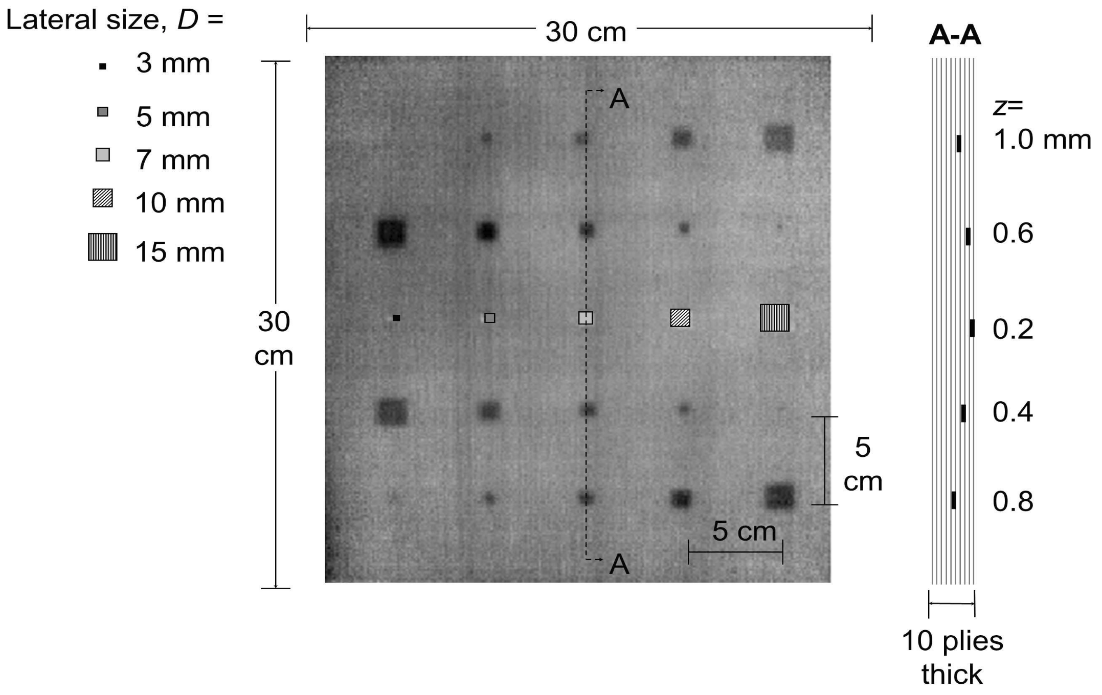
In order to evaluate the potential interest of ICA in IRNDT, we analyzed a reference Carbon Fiber Reinforced Plastic (CFRP) sample. We used the same sample as Erazo et al. [93]. This sample contains twenty-five Teflon inserts which are divided into five sets of five defects. Each set has five inserts having the same depth but different sizes (from 3 × 3 mm 2 to 15 × 15 mm 2 ). As illustrated in Figure 2, each set has been positioned at a specific depth (from 0.2 to 1 mm).
The materials are evaluated under a classic pulsed thermography procedure.
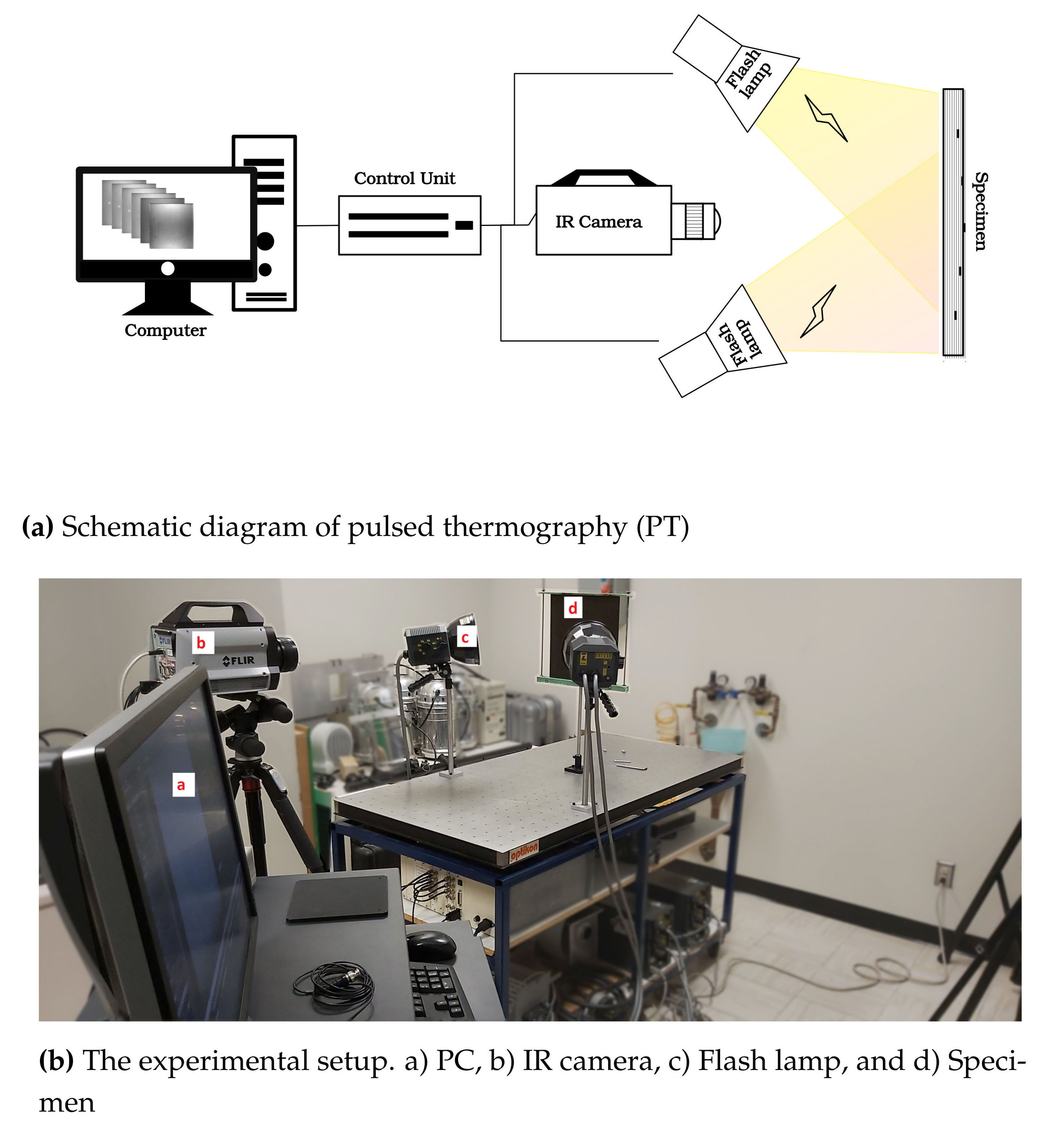
Pulsed thermography (PT), shown in Figure 3a, consists of an external heating source and an Infrared camera. A short pulse of energy from the heating source is emitted to the surface of the specimen. The temperature decay is then captured from an excited surface using the IR camera. Because we are using two flashes, a control unit was required to control and synchronize the data acquisition with flash triggering. The acquired thermal sequences were stored on a computer. From a more theoretical point of view according to the general heat Equation [123]:
2 T y 2 = 1 μ d T d t
where T is the surface temperature, μ = k / ρ c p is the thermal diffusivity of the material, k, ρ , and c p its thermal conductivity, density, and specific heat at constant pressure, respectively; t is the time, and y is the depth of the specimen. The 1D solution of the Fourier Equation with ideal waveform and for homogeneous and semi-infinite material is given by Equation (21):
T ( y , t ) = E e π t e y 2 4 μ t
where E is the absorbed energy by the surface and e is the heat effusivity ( e = ( k ρ c p ) 1 / 2 ). The emitted energy from the surface where y = 0 (Equation (22)) represents temperature change after applying heat to the surface of the specimen.
Δ T ( t ) = E e π t
Each material has been stimulated from the front side by a pulse generated by two photographic flashes (5 ms thermal pulse, 6.4 kJ/flash (Balcar, France)). A mid-wave infrared (MWIR) camera FLIR x6900sc (1.5 μm to 5.0 μm, 14 bit per pixel, 640 × 512 ) was used for data acquisition. We conducted two acquisitions at different frequencies of acquisition. We acquired some data at a frequency of 145 Hz (145 images per second) and 120 Hz for 30 s. That duration ensured that the sensor had acquired both the warm-up and the cool-down. Then, we sub-sampled them to a sequence of 2000 frames and 2200 frames, respectively.

4.2. Analysis

In this study, we investigated different aspects regarding the usage of the Independent Component Analysis. We chose to compare the results of our experiments with two state-of-the-art methods, the PPT [8], and the PCT [9]. We conducted three investigations regarding the importance of selecting the component on the accuracy of the results, evaluating the different methods we selected, and finally, the influence of the acquisition frequency on our data’s accuracy. The first aspect of our study concerns the selection of the number of components. Several papers have been published offering methods regarding selecting the number of components regarding different applications optimally. Although the work of Rengifo et al. [119] fits our goals, they used a nonquadratic activation function given in Equation (10) and developed a method to identify the most suitable independent component for detecting defects. However, this method can not be generalized for other activation functions; thus, we chose not to use it in our study. Therefore we conducted a limited study regarding the importance of selecting the proper number of components for ICA. For each method under investigation and each dataset, we reduced the dimensionality to one hundred and seven components. The numbers seven and one hundred were randomly selected. We compute the CNR for both cases and every defect. Then the results for seven and one hundred components are compared.
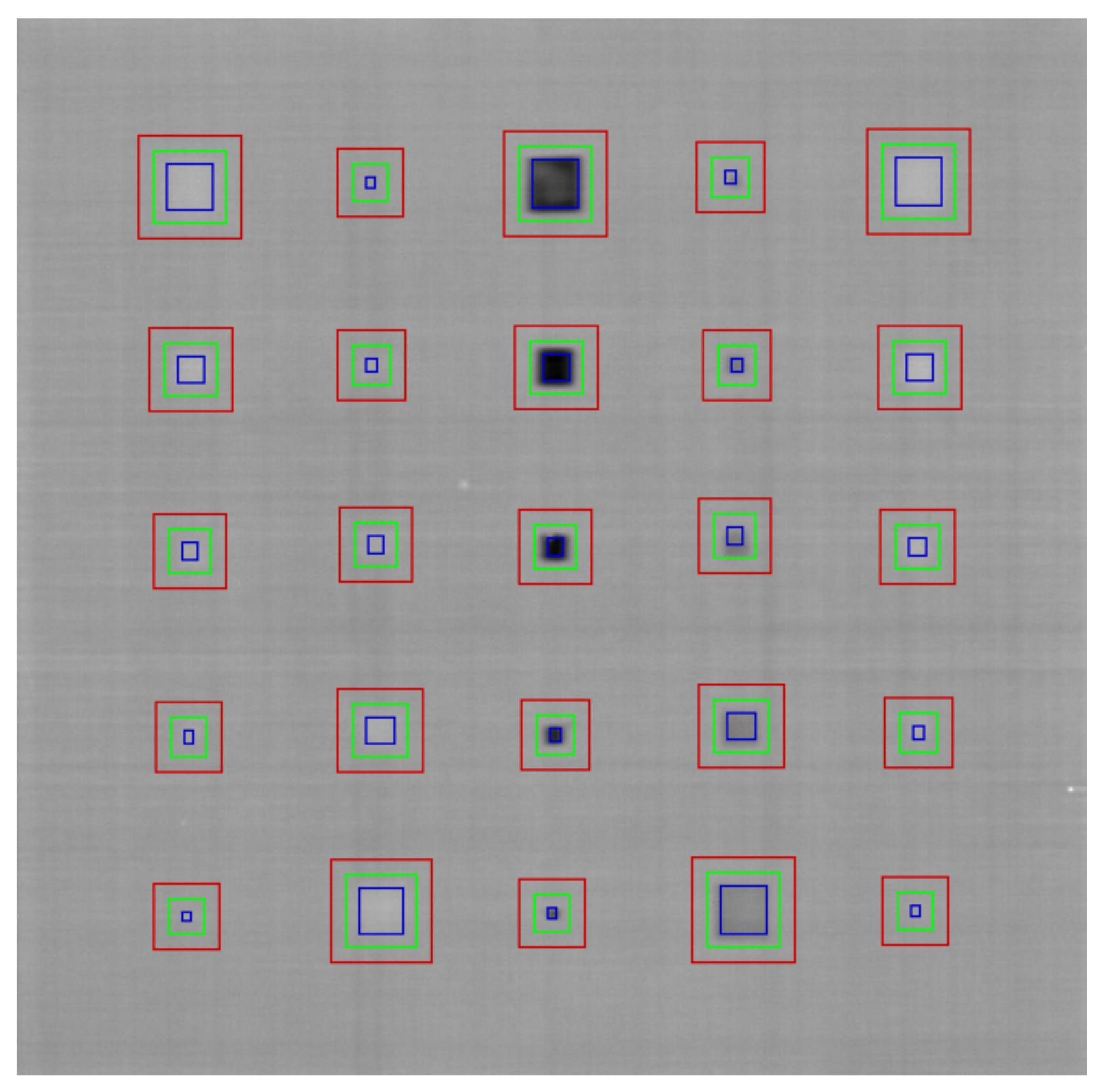
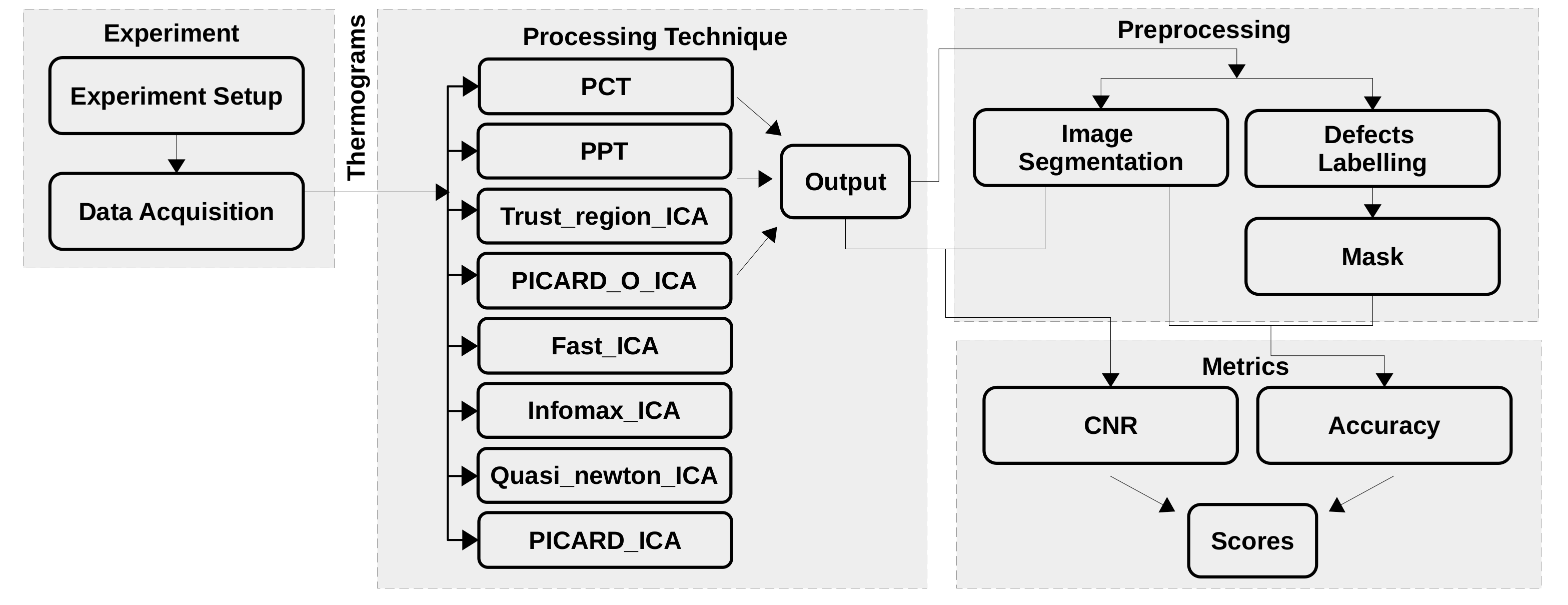
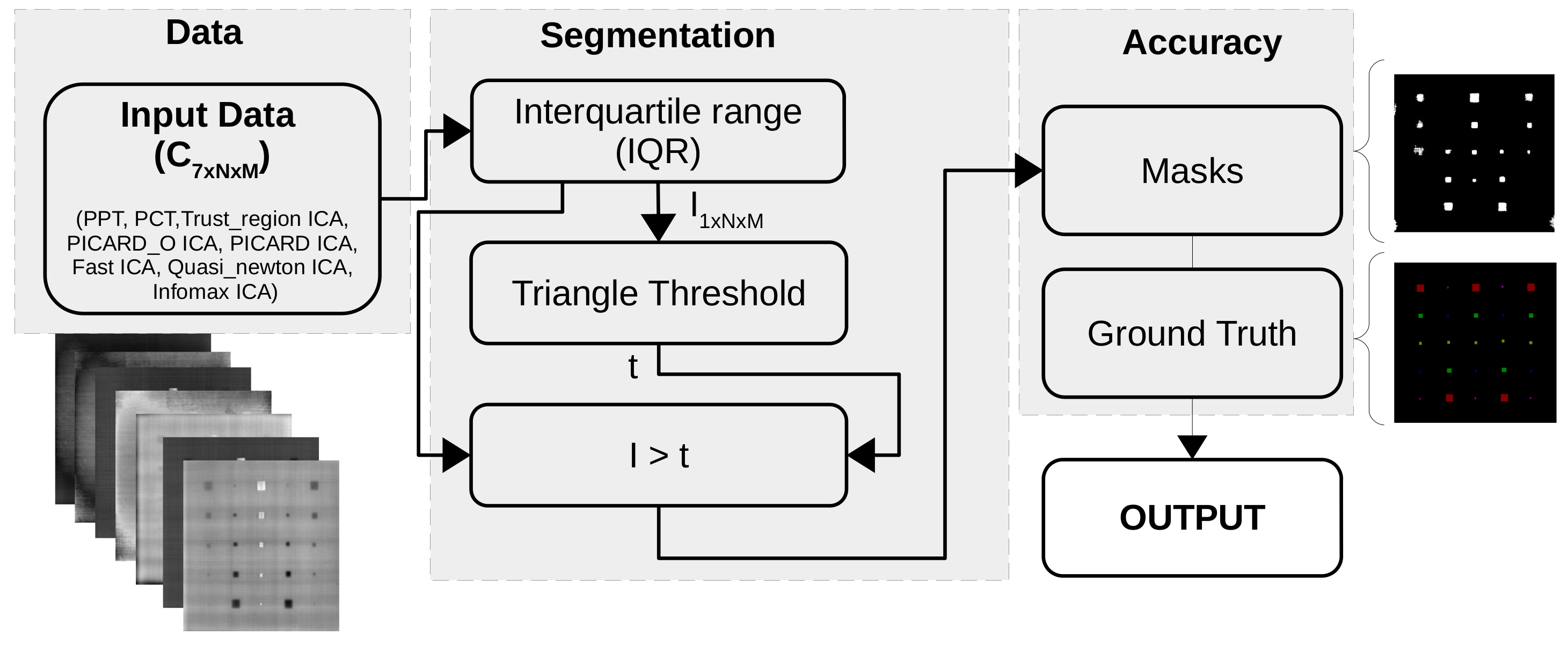
Then for a given defect we identify the frame with the highest CNR score, which we report in our results. For each defect, the CNR is computed for a region of interest representing the defective region and a region of interest used as a sound area, as one can note in Figure 4. One can note that the sound area overlaps the defective region, it is obvious that for the computation of the CNR all overlapping pixels were not considered part of the sound area. For evaluation of all selected methods, we use CNR values of seven components. For the PPT the CNR values were computed the same manner as those of the ICA’s methods. Figure 5 shows the different step of our experiment. Another aspect of the evaluation of the different methods concerns their ability, when coming to the segmentation task, is to provide an accurate mask of the defects present in the sample. Inspired by Feng et al. [72], to construct a single image from the several components or phase images, we compute the InterQuartile Range (IQR) for each pixel of selected outputs. Then, from this image, we used the triangle automatic threshold method [124] to compute an optimal threshold, which is applied to the previous image to generate a mask of the defects. We thus estimated the accuracy based on these images and compare it with other methods. Figure 6 shows the different steps of this experiment. To conclude our study we compare the results we computed from each method between the different acquisition frequencies.
Before any analysis, we first need to pre-process the sequence we acquired. We acquired a sequence of T images of M × N pixels that are structured as a third-order tensor for each frequency. The first step consists in creating an overlay matrix of dimension T × P where P = M . N . T is the number of frames acquired in each sequence, P is the total number of pixels. Figure 7 shows that operation.
As preprocessing we standardized the overlay matrix. To do so we compute the mean and standard deviation of each column of the matrix, thus for each row of the matrix we subtract the mean vector previously computed and divide it by the standard deviation vector. In the next section, we introduce the metrics we use for assessing the quality of the different methods we investigated.

4.3. Figure of Merit

To evaluate the different aspects of out study we choice two figures of merit, the CNR and the Accuracy. The first metric we introduce is quite well-known in Infrared Non-Destructive Testing (IRNDT), it is the Contrast to Noise Ratio (CNR).

4.3.1. CNR

This metric allows evaluating the general contrast of the defective region regarding the surrounding. CNR is prevalent in IRNDT due to its ability to provide information about the image’s contrast. Often, thermal or component images are noisy, which can significantly influence this metric. Many formulations of the CNR have been proposed; in this study, we used the formulation proposed by Usamentiaga [125].
C N R ( r o i s , r o i n ) = μ s μ n ( σ s 2 + σ n 2 ) 2
where μ s and μ n represent the mean of the sound area and the defect area’s mean, respectively. σ s and σ n represent the standard deviation of each region. In the next section, we briefly introduce another figure of merit, Accuracy.

4.3.2. Accuracy

Accuracy is a common metric. It is a very helpful metric to evaluate the quality of detection and segmentation. Its definition for a binary classifier is define by Equation (24).
A c c u r a c y = T P + T N T P + T N + F P + F N
where TP (i.e., True Positive) represents the number of pixels detected that were truly part of the ROI. TN (i.e., True Negative) represents the number of pixels that were accurately detected as part of the background. FP (i.e., False Positive) represents the number of wrongly detected pixels as part of the ROI. FN (i.e., False Negative) is the number of wrongly detected pixels as part of the background. Figure 8 provides a visual example.
Illustration of the different concepts used in Receiver Operating Characteristic approaches.
The following section introduces the different results we computed for this study.

5. Results

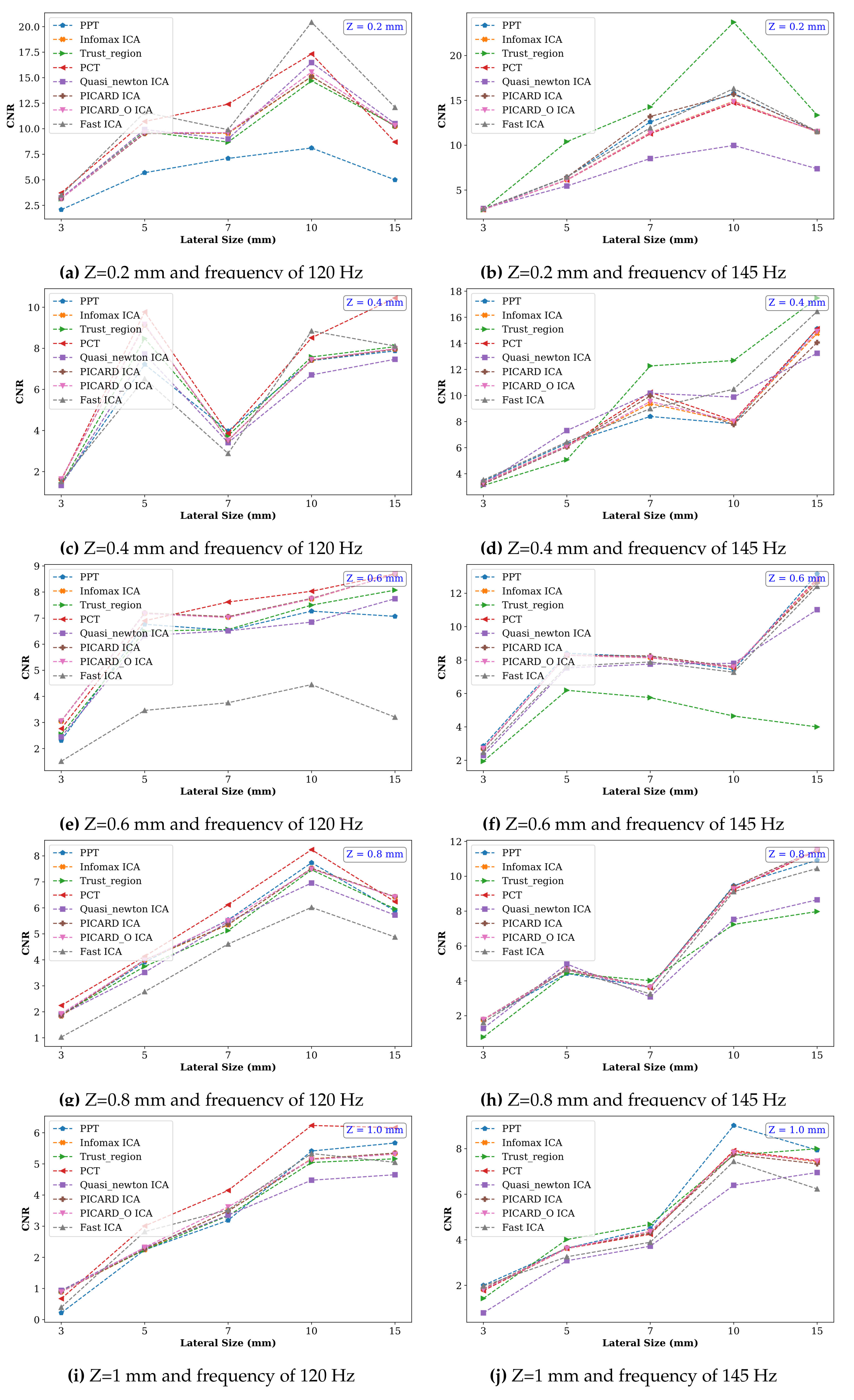
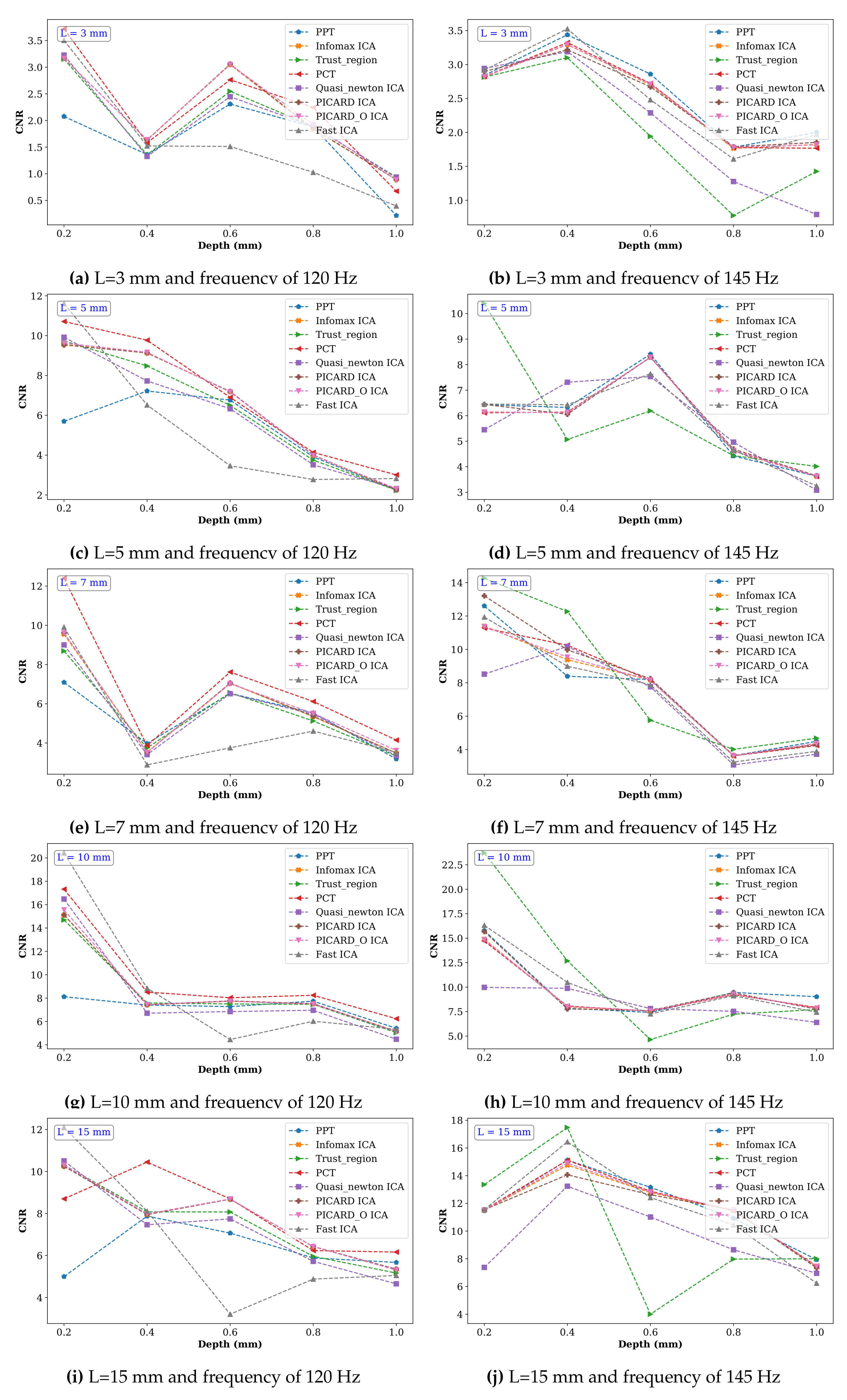
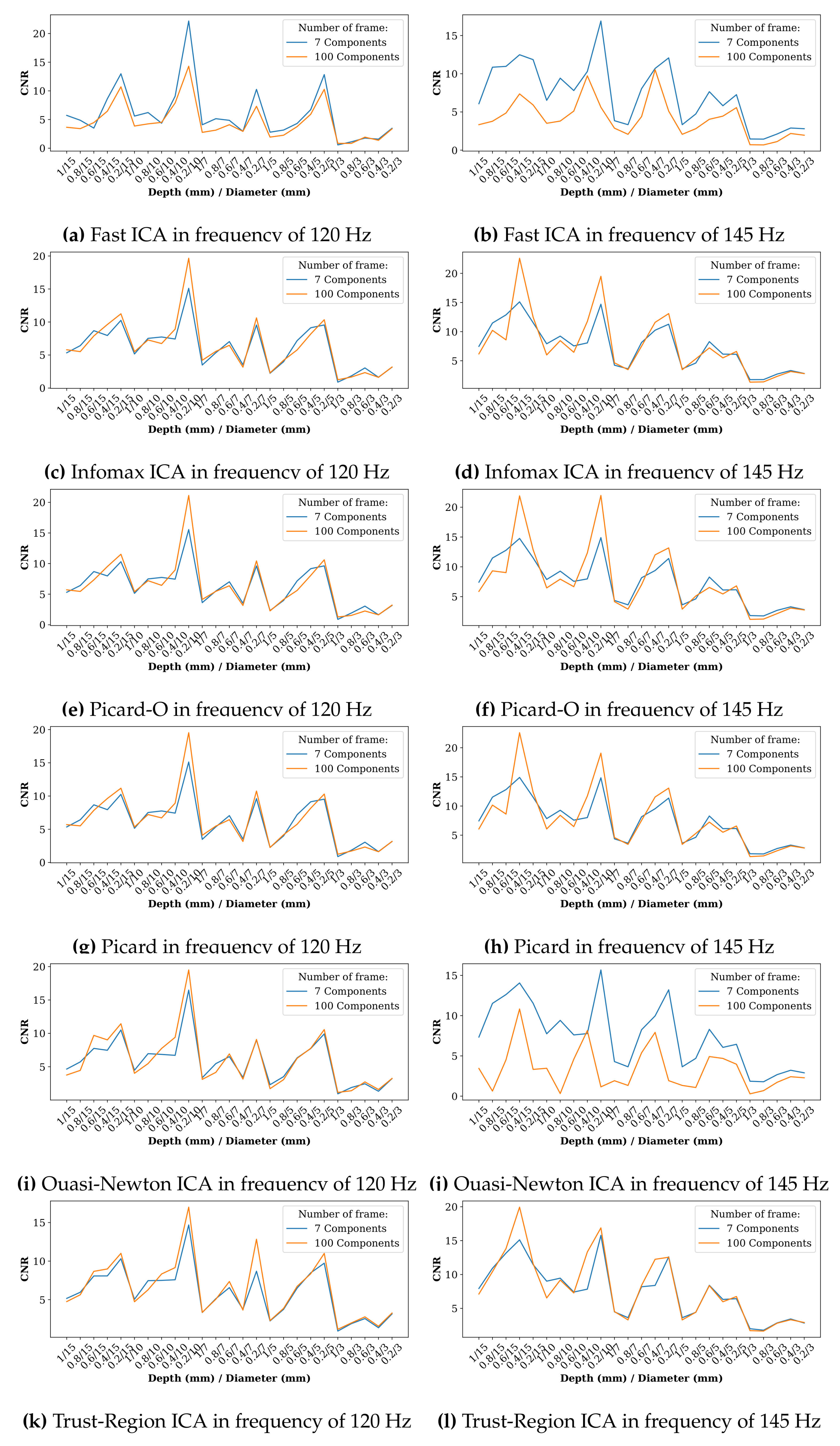
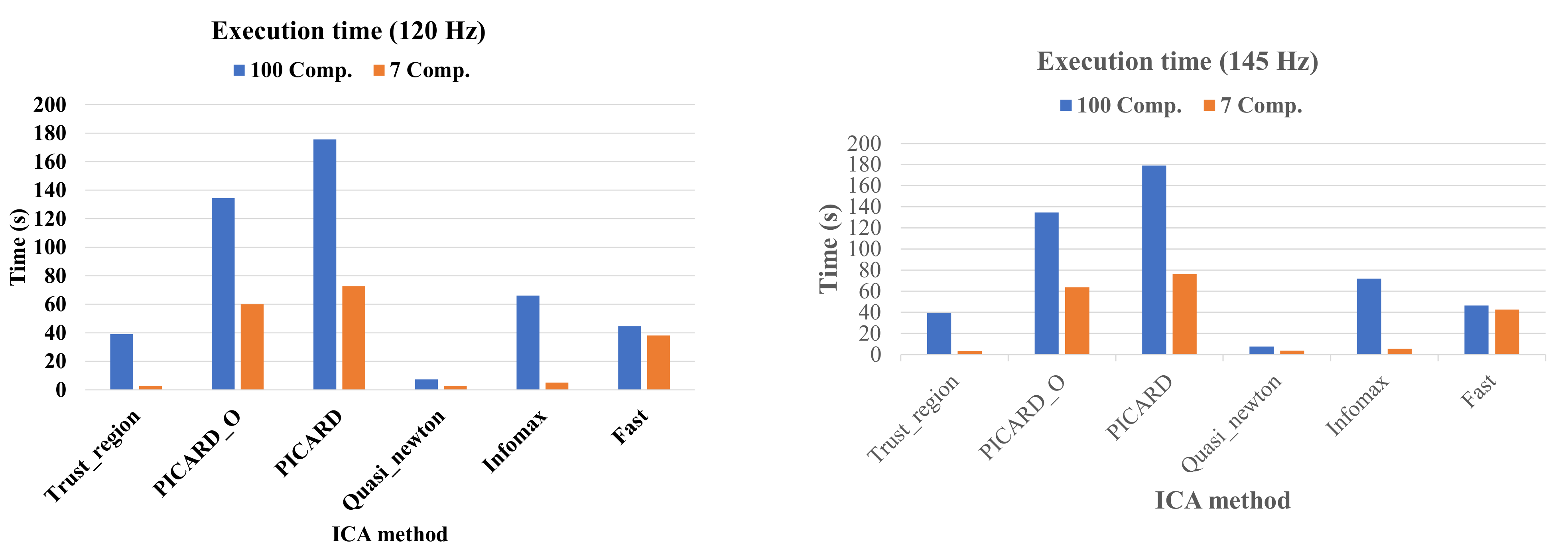
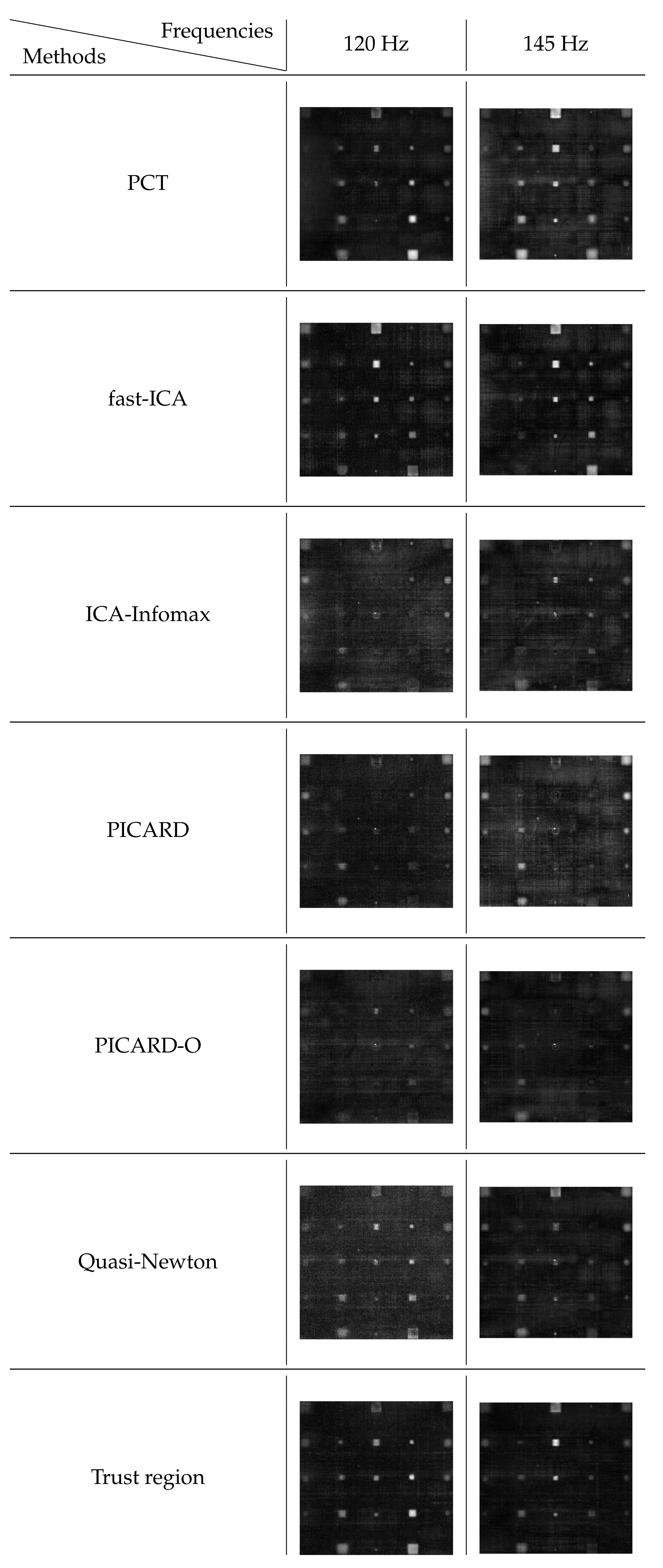
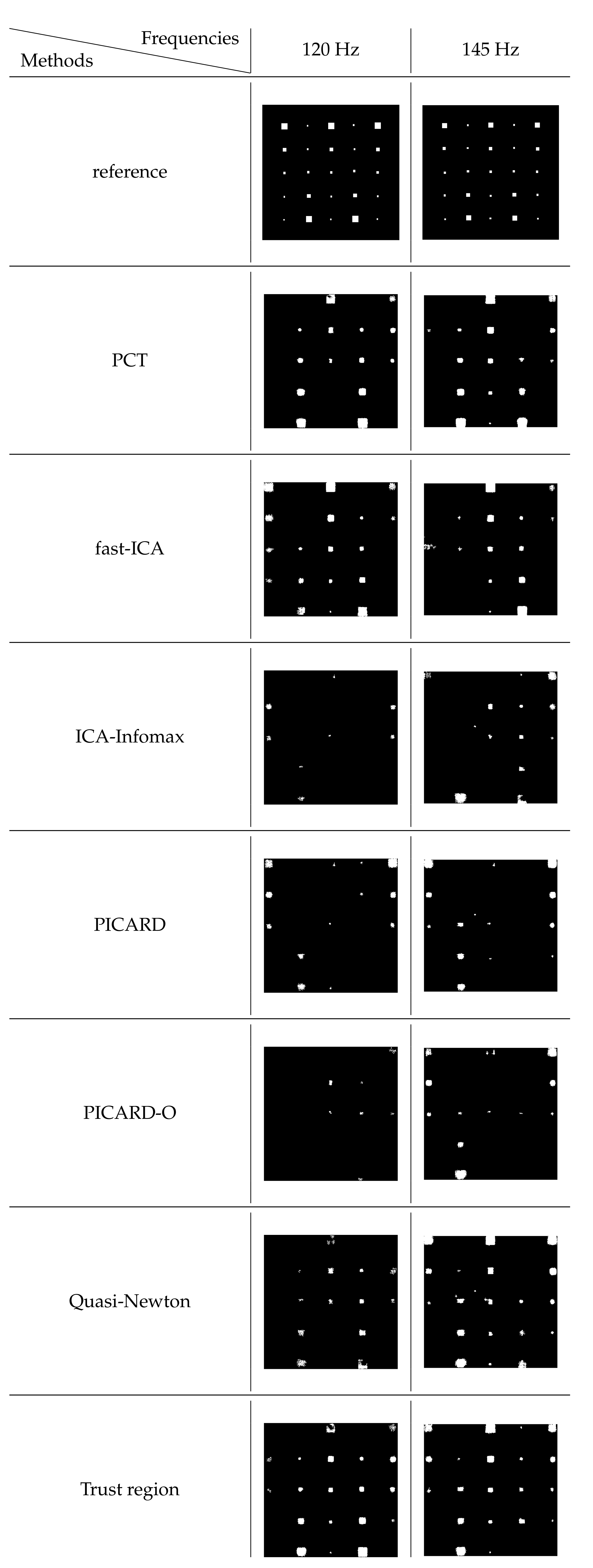
Regarding the experiments we conducted to evaluate and the different ICAs methods we selected with the PPT and PCT. For each method we reported the CNR scores of each defect in Table 2 In that tab for each method the first column represents the depth of the defect, the second and third columns shows for a given lateral size defects the max CNR obtained at each depth for the two datasets we used. The next column introduce percentage of difference between the two results. A negative sign is given to the difference when the max CNR obtained for the dataset acquired at the frequency of 145 Hz are lower than the results obtained for the dataset acquired at 120 Hz. This columns pattern is used for all the defect size. In Figure 9 each plot shows the maximum CNR scores obtained by each method for the different defect size, for a given depth and a given frequency. Similarly in Figure 10 each plot show the maximum CNR scores obtained by each method for the different depth, for a given lateral size and a given frequency. For the experiments about the importance of the number of the components on the defect identification. We computed the CNR for 7 and 100 components for different ICA methods. Figure 11 presents the maximum CNR value for all defects in different depth and size. We also computed for the two frequencies of acquisition investigated, the mean sequences for the ICA methods; i.e., the mean of the sequences computed for each method, for one hundred components and seven components respectively. We show the result of the computation of the inter quantile range on each mean sequences in Figure 12. Table 3 and Figure 13 show the computation time of the different methods we used for each experiment we conducted. The results for the Accuracy scores using the segmentation approach describe in Section 4.2 and illustrated in Figure 6 are reported in Table 4. Regarding the experiments about segmentation we plot the results of both the application of the IQR per pixel on the result of the different methods in Figure 14. We also plot the result mask computed using the proposed segmentation approach in Figure 15.
Table 3 summarizes the processing time for all ICA methods.
In the next section, we discuss the results we obtained.

6. Discussion

The goal of this study was to investigated the performances of different ICA algorithms for processing PT data. We chose two state-of-the-art methods in order to provide a fair comparison. This study focus on three features, the contrast of each defects with its closest neighbourhood, the accuracy of detection for a given segmentation algorithm, and the time of execution. We investigated these feature using two dataset of the same samples acquired with different frequencies, which allow us to extend also observe the influence of the frequency of acquisition on the three features we investigated. For each case we provide quantitative results.
From Table 2 we can observe that for most of the methods investigated, the CNR for the defect from the sequence acquired at 145 Hz offers a higher CNR than at 120 Hz. The highest difference are observed for the PPT where for 80% of the defects have a higher CNR at 145 Hz than 120 Hz. Quasi-newton and Trust-region-ICA shows a higher CNR at 145 Hz for 76% of the defects. 72% of the defects have a higher CNR at 145 Hz with the Fast-ICA method. Infomax-ICA, PICARD and PICARD-O have better CNR at 145 Hz for 68% of the defects. PCT shows 60% of the defects have a higher CNR at 145 Hz.
For the data acquired at the frequency of 120 Hz we made the following observations. The defects with a lateral size of 3 mm, have a higher CNR for 60% of the ICA method compared with PCT. Five over six investigated ICA methods offer higher CNR than PPT. The same number of methods outperform the PCT regarding the CNR for the defect with the smallest lateral size, located at the deepest depth (L = 3 mm, d = 1 mm). For this particular defect all the ICA methods outperformed the PPT. The best CNR is obtained by the Quasi-Newton approach. We can observe that for smaller and shallowest PCT exceeds both ICA and PPT. The differences between ICAs methods and PCT regarding the scores vary from 7% to 17% lower. PPT reaches the highest difference ratio with PCT with a score of 79% lower. PCT, PPT, and ICA methods have higher CNR values for 60%, 4%, and 36% of the defects. Among the ICAs method the best results were obtained by Fast-ICA and PICARD methods. As one can note ICAs methods except for smaller and deeper defects does not better than the PCT method. However, ICAs CNR results are often close to those of the PCT. For the experiment conducted with the data acquired at the frequency of 145 Hz, we observed that the ICAs method exceed PPT and PCT for 72% of the defects. PCT and PPT beat the ICAs methods for 12% and 16% of the defects, respectively. For deeper and smaller defects, Trust-region ICA beats both PPT and PCT. Nonetheless, the increase in CNR, even if slightly higher, is similar to PCT. One can note that ICA methods are better than state-of-the-art approaches for deeper defects. For the shallowest defects (depth = 0.2 mm), the CNR scores for the ICAs methods are quite close regardless of the method. Similar observations can be made for the defects with a lateral size of 3 mm located at a depth of 0.2 mm and a depth of 0.4 mm, for all the methods. Between ICA methods, Trust ICA, Fast ICA, Quasi-newton ICA, and PICARD in 64%, 16%, 16%, and 4% of defects has the maximum CNR, respectively. Among all the methods, Trust ICA, Quasi-Newton ICA, Fast ICA, PPT, and PCT obtained 32%, 24%, 16%, 16%, and 12% of the maximum CNR scores, respectively.
As mentioned in Section 4.2 we conducted a limited investigation about the selection of the components. In this investigation we computed for each component method 100 components as well as 7 components. Then for each case we compute the maximum CNR for each defects and compare the results. As one can note in Figure 11 for most of the methods regardless the number of component we found that there is no significant variation between the maximum CNR computed for 7 components and the one computed for 100 components. We can see in plots Figure 11b,j a noticeable difference between the two max CNR in terms of amplitude. In both cases the CNR computed for 7 components offers higher amplitude than the one computed for one hundred components. For both cases the shape of the plot are quite similar, nevertheless we can surprisingly observe a slight offset of the maximum CNR. Other less significant difference between the maximum SNR computed for 7 and 100 component are visible for some of the other plot. For most of the other methods despite a slight difference regarding the amplitude the shape of the plot are very similar and does not shows any offset. One can note that the difference between CNR are higher for the data acquired at 145 Hz than at 120 Hz. Looking at Table 3 and Figure 13 one can note that computing a higher number of component increases the execution time, especially regarding for Trust-region ICA and infomax ICA, where the computation time for 100 components 13 times slower than the one for 7 components at frequency 120 Hz. Fast ICA for 7 and 100 components are quite close, 1.17 and 1.09 time slower at frequency of 120 Hz and 145 Hz, respectively. For other ICA methods the difference between computing 7 components and 100 varies from 2.24 to 13.74 times slower at a frequency of 120 Hz, and from 2.03 to 13.16 times slower at 145 Hz. Although Trust-region ICA and quasi-newton ICA offers among the quicker computation time between the ICAs methods, the number of component to compute does not affect their computational time equally. Even method such as PCT which is on PCA that is nowadays a highly optimized algorithm needed two times more time to compute 100 components that 7. Surprisingly we observed that all the methods had a quicker computational time on the data acquired at 120 Hz than 145 Hz. To conclude our investigation regarding the influence of the number of components on the results we computed for each dataset, for both 100 components and 7 components, the mean of the components of all the methods. For a given number of components we computed obtain 6 results, 1 for each method. For simplification we suppose that the result of each method is a third rank tensor, where the first dimension correspond to the number of components, the two other dimensions represents the number of rows and columns respectively of each components. In order to compute the mean component we compute for a given components index the mean of the results for this index. Once the all the mean of the component have computed for all the component index we compute IQR for every matrix coordinates. The result obtained is a matrix of the same number of rows and columns as the component. Figure 12 shows the results we obtained, which leads us to the conclusion that fewer component offer a higher contrast regarding the defective region and therefore makes it easier to identify them.
Another investigation we conducted in our study regards the ability of each method to provide a distinctive output for automatic segmentation. To do our experiments we used the algorithm introduces in Figure 6. Table 4 shows the accuracy score computed from the segmented images showed in Figure 15. We also show in Figure 14 the result of the computation of the IQR per pixel from the output of the different methods. The accuracy was compute for each defects separately and then averaged. We can observed that the results regarding the segmentation varies a lot from a method to another. The accuracies scores shows that both Trust-region-ICA as well as Fast-ICA outperform PCT for the data acquired at 120 Hz. We can see that PCT segmentation does not perform well for defects located at 1 mm, for the smallest defects as well as for defects with a lateral size of 5 mm located at a 0.2 and 0.4 mm from the surface. Fast-ICA method performs better than PCT for smaller defects, but miss the smallest defect located a depth deepth than 0.2 mm. Interestingly the defects with a lateral size lower than 10 mm located at a depth 0.8 mm are not detected while defects located at the depth of 1 mm with a lateral size of 10 mm as well as 5 mm are partially detected. Trust-Region-ICA shows more consistant results than PCT and Fast-ICA. This method was able to detect even partially all the defects located a depth of 0.2 mm. All but the smallest defect for the depths of 0.4 mm, 0.6 mm, and 0.8 mm from the surface. It was able to made two partial detection for the defect with a lateral size of 10 mm and 7 mm located at the depth of 1 mm from the surface. Quasi-Newton-ICA offers similar results compared with PCT. Nonetheless most of the detection most of the detection made with this methods are partial, unlike PCT. ICA-Infomax, PICARD, PICARD-O, does shows many detection mostly partial. The number of detection as well as the quality of detection does make these method uninteresting for defect detection. In short for the data acquired at 120 Hz, the segmentation approach shows that Fast-ICA algorithm outperform all the other method regarding the segmentation of defects locate a the depth of 1 mm from the surface while Trust-region-ICA is the method that has detected the highest number of defects. For the data acquired at 145 Hz the results of the segmentation shows that the PCT offers similar results as previously observed. Fast-ICA method underperform for defect located at depth lower than 0.4 mm from the surface, compared with the results obtained with the data acquired at 120 Hz. Trust-region-ICA offers better performances for the defect located at a depth of 1 mm from the surface but fails for this depth to detect the smallest defect. It also fails to detect the largest defect located at the depth of 0.4 mm from the surface, while being able to detect all the other defects. For the rest of the defect the performance of Trust-region-ICA are mostly similar to what has been present for the data acquired at 120 Hz. Quasi-Newton-ICA result improved noticeably. It is able to detect all the defects of the shallowest depth, and for the other depth all the defects with a lateral size from 7 mm and higher. It is also able to detect the defect with a lateral size of 5 mm located at a depth of 0.8 mm. It shows also some partial detection in non defective region. ICA-Infomax, PICARD, PICARD-O, shows better results on the data acquired at 145 Hz than they did on the previous data. In spite of these improvement these methods shows very poor results compaired with the other methods. To sum up, on the data acquired at a frequence of 120 Hz both Fast-ICA and Trust-region-ICA performed well compared with PCT. On the data acquired at a frequence of 145 Hz, Fast-ICA’s underperformed while Quasi-Newton-ICA performances were improved. Trust-region-ICA results were quite similar.
To conclude the different aspect of our study, we have observed that for most of the method we investigated computing a smaller number of components does not significantly affect the CNR results. Have fewer component can makes the identification of the defects in the sample easier. The number of component to compute can significantly affect the computation depending the method. Using a simple segmentation approach in association with the accuracy score we also showed that the frequence of acquisition can significantly affect the results of some algorithms. Among those we investigated Fast-ICA, Trust-region-ICA and Quasi-Newton ica provided consistent output, while have a reasonable computational time.

7. Conclusions

This paper has three contributions. First of all, we reviewed the most recent works regarding the processing of CFRP samples tested by PT. Secondly, because dimensional reduction methods are very popular in IRNDT, we investigated the influence of the number of components on the results from a quantitative and qualitative perspective. We limited our study to PCT and several ICA methods selected among the recent works. We compared the CNR in each defect for when we used seven and hundred components. Our results show that for each method when one hundred components are computed the CNR per defect is not noticeably higher than for seven components. Similarly, the trends regarding the evaluation of the CNR per surface and depth are the same. From a detection point of view, having many components makes it harder to find accurate and reliable segmentation methods without supervised learning. Some strategies based on simple statistics, such as the interquartile range, or the kurtosis, may provide a quasi-accurate segmentation method with fewer components. In our third contribution, we quantitatively compare the selected ICAs algorithm with PCT and PPT. Our results show that in most of the cases ICAs method outperformed PPT, but not PCT. However, for smaller defects and deeper defects ICAs method often outperforms PCT. The results also show that if ICAs results are generally not far from the one of the PCT.
Further research would involve supervised ICA algorithms, feature enhancement methods [15], and the unsupervised ICA method in this research on a wider range of materials.

Author Contributions

Conceptualization, J.R.F., S.E., C.I.-C. and X.P.V.M.; methodology, J.R.F. and S.E.; software, J.R.F. and S.E.; validation, J.R.F. and S.E.; formal analysis, J.R.F. and S.E.; investigation, J.R.F. and S.E.; data, C.I.-C.; data curation, J.R.F. and S.E. All authors have read and agreed to the published version of the manuscript.

Funding

This research is funded by the NSERC DG program and Canada Research Chair Program (MIVIM Multipolar Infrared Vision Infrarouge Multipolaire).

Institutional Review Board Statement

Not applicable.

Informed Consent Statement

Not applicable.

Data Availability Statement

Data sharing not applicable.

Acknowledgments

The authors would like to thank Annette Schwerdtfeger for the time and energy she spent reviewing this article.

Conflicts of Interest

The funders had no role in the design of the study; in the collection, analyses, or interpretation of data; in the writing of the manuscript, or in the decision to publish the results.

Abbreviations

The following abbreviations are used in this manuscript:
NDTNon Destructive Testing
IRTInfraRed Thermography
PTPulsed Thermography
PPTPulsed Phase Thermography
PCAPrincipal Component Analysis
PCTPrincipal Component Thermography
ICAIndependent Component Analysis
ICTIndependent Component Thermography
BSSBlind Signal Seperation
CFRPCarbon Fiber Reinforced Plastic
CNRContrast over Noise Ration
MoGMixture of Gaussian
CCIPCACandid Covariance-free Incremental Principal Component Analysis
CCIPCTCandid Covariance-free Incremental Principal Component Thermography
ESPCAEdge-group Sparse Principal Component Analysis
ESPCTEdge-group Sparse Principal Component Thermography
Sparse-PCASparse Principal Component Analysis
SPCTSparse Principal Component Thermography
NMFNon-negative Matrix Factorization
LatLRRLatent Low Rank Representation
LatLRRTLatent Low Rank Representation in Thermography
PLSPartial Least Square
PLSTPartial Least Square Thermography
TSRThermographic Signal Reconstruction
SVMSupport Vector Machine
OLPPTOrthogonal Locally Preserving Projection Thermography
ANNArtificial Neural Network
DTTDynamic Thermal Tomography
GSAGapped Smoothing Algorithm
DACDifference of Absolute Contrast
MDACModified Difference of Absolute Contrast
ATIApparent Thermal Inertia
TQThermal Quadrupole
NLFNon Linear Fitting
GANGenerative Adversarial Network
LWIRLong Wavelength InfraRed
MWIRMid Wavelength InfraRed
KPCAKernel-PCA
HOGHistogram of Oriented Gradient.

References

  1. Meola, C.; Boccardi, S.; Carlomagno, G.M. Infrared Thermography in the Evaluation of Aerospace Composite Materials: Infrared Thermography to Composites; Woodhead Publishing: Sawston, UK, 2016. [Google Scholar]
  2. Vavilov, V.; Burleigh, D. Infrared Thermography and Thermal Nondestructive Testing; Springer: Berlin, Germany, 2020. [Google Scholar]
  3. Houchin, J.S.; Parulski, K.A. Calibration System for a Raster Input Scanner. U.S. Patent 5,047,861, 10 September 1991. [Google Scholar]
  4. Harris, J.G.; Chiang, Y.M. Nonuniformity correction of infrared image sequences using the constant-statistics constraint. IEEE Trans. Image Process. 1999, 8, 1148–1151. [Google Scholar] [CrossRef] [Green Version]
  5. Ratliff, B.M.; Hayat, M.M.; Tyo, J.S. Radiometrically accurate scene-based nonuniformity correction for array sensors. JOSA A 2003, 20, 1890–1899. [Google Scholar] [CrossRef] [Green Version]
  6. Perenzoni, M.; Mosconi, D.; Stoppa, D. A 160 × 120-pixel uncooled IR-FPA readout integrated circuit with on-chip non-uniformity compensation. In Proceedings of the 2010 IEEE ESSCIRC, Seville, Spain, 14–16 September 2010; pp. 122–125. [Google Scholar]
  7. Cao, Y.; Tisse, C.L. Single-image-based solution for optics temperature-dependent nonuniformity correction in an uncooled long-wave infrared camera. Opt. Lett. 2014, 39, 646–648. [Google Scholar] [CrossRef]
  8. Maldague, X.; Marinetti, S. Pulse phase infrared thermography. J. Appl. Phys. 1996, 79, 2694–2698. [Google Scholar] [CrossRef]
  9. Rajic, N. Principal Component Thermography; Technical Report; Defence Science and Technology Organisation: Victoria, Australia, 2002. [Google Scholar]
  10. Hyvärinen, A.; Karhunen, J.; Oja, E. Independent Component Analysis. In Adaptive and Cognitive Dynamic Systems: Signal Processing, Learning, Communications and Control; Wiley: Hoboken, NJ, USA, 2004. [Google Scholar]
  11. Liu, Y.; Wu, J.Y.; Liu, K.; Wen, H.L.; Yao, Y.; Sfarra, S.; Zhao, C. Independent component thermography for non-destructive testing of defects in polymer composites. Measur. Sci. Technol. 2019, 30, 044006. [Google Scholar] [CrossRef]
  12. Fleuret, J.; Ebrahimi, S.; Maldague, X. Pulsed Thermography Signal Reconstruction Using Linear Support Vector Regression. In Proceedings of the 2020 International Conference on Quantitative InfraRed Thermography, Porto, Portugal, 6–10 July 2020. [Google Scholar] [CrossRef]
  13. Ahmed, J.; Gao, B.; Tian, G.Y.; Yang, Y.; Fan, Y.C. Sparse ensemble matrix factorization for debond detection in CFRP composites using optical thermography. Infrared Phys. Technol. 2018, 92, 392–401. [Google Scholar] [CrossRef]
  14. Zhang, X.; Saniie, J.; Heifetz, A. Neural learning based blind source separation for detection of material defects in pulsed thermography images. In Proceedings of the 2020 IEEE International Conference on Electro Information Technology (EIT), Chicago, IL, USA, 31 July–1 August 2020; pp. 112–116. [Google Scholar]
  15. Liu, K.; Tang, Y.; Lou, W.; Liu, Y.; Yang, J.; Yao, Y. A thermographic data augmentation and signal separation method for defect detection. Measur. Sci. Technol. 2021, 32, 045401. [Google Scholar] [CrossRef]
  16. Netzelmann, U.; Müller, D. Modified pulse-phase thermography algorithms for improved contrast-to-noise ratio from pulse-excited thermographic sequences. NDT E Int. 2020, 116, 102325. [Google Scholar] [CrossRef]
  17. Vavilov, V.P.; Shiryaev, V.V.; Kuimova, M.V. Time-and phase-domain thermal tomography of composites. Photonics 2018, 5, 31. [Google Scholar] [CrossRef] [Green Version]
  18. Poelman, G.; Hedayatrasa, S.; Segers, J.; Van Paepegem, W.; Kersemans, M. Adaptive spectral band integration in flash thermography: Enhanced defect detectability and quantification in composites. Compos. Part B Eng. 2020, 202, 108305. [Google Scholar] [CrossRef]
  19. Ahmed, J.; Baloch, G.A.; Tian, G.Y. Wavelet Domain Based Defect Detection using Optical Thermography. In Proceedings of the 2019 International Conference on Intelligent Medicine and Image Processing, Bali, Indonesia, 19–22 April 2019; pp. 83–87. [Google Scholar]
  20. Ahmed, J.; Gao, B.; Woo, W.L. Wavelet-integrated alternating sparse dictionary matrix decomposition in thermal imaging CFRP defect detection. IEEE Trans. Ind. Inf. 2018, 15, 4033–4043. [Google Scholar] [CrossRef]
  21. Ahmed, J.; Gao, B.; Woo, W.L.; Zhu, Y. Ensemble Joint Sparse Low-Rank Matrix Decomposition for Thermography Diagnosis System. IEEE Trans. Ind. Electron. 2020, 68, 2648–2658. [Google Scholar] [CrossRef]
  22. Liu, L.; Gao, B.; Wu, S.; Ahmed, J.; Woo, W.L.; Li, J.; Yu, Y. Structured iterative alternating sparse matrix decomposition for thermal imaging diagnostic system. Infrared Phys. Technol. 2020, 107, 103288. [Google Scholar] [CrossRef]
  23. Yousefi, B.; Sfarra, S.; Castanedo, C.I.; Maldague, X.P. Comparative Analysis on Thermal Non-Destructive Testing Imagery Applying Candid Covariance-Free Incremental Principal Component Thermography (CCIPCT). Infrared Phys. Technol. 2017, 85, 163–169. [Google Scholar] [CrossRef]
  24. Weng, J.; Zhang, Y.; Hwang, W.S. Candid Covariance-Free Incremental Principal Component Analysis. IEEE Trans. Pattern Anal. Mach. Intell. 2003, 25, 1034–1040. [Google Scholar] [CrossRef] [Green Version]
  25. Wu, J.Y.; Sfarra, S.; Yao, Y. Sparse principal component thermography for subsurface defect detection in composite products. IEEE Trans. Ind. Inf. 2018, 14, 5594–5600. [Google Scholar] [CrossRef]
  26. Yousefi, B.; Sharifipour, H.M.; Castanedo, C.I.; Maldague, X.P. Automatic IRNDT inspection applying sparse PCA-based clustering. In Proceedings of the 2017 IEEE 30th Canadian Conference on Electrical and Computer Engineering (CCECE), Windsor, ON, Canada, 30 April–3 May 2017; pp. 1–4. [Google Scholar]
  27. Wen, C.M.; Sfarra, S.; Gargiulo, G.; Yao, Y. Edge-Group Sparse Principal Component Thermography for Defect Detection in an Ancient Marquetry Sample. Proceedings 2019, 27, 7034. [Google Scholar] [CrossRef] [Green Version]
  28. Wen, C.M.; Sfarra, S.; Gargiulo, G.; Yao, Y. Thermographic Data Analysis for Defect Detection by Imposing Spatial Connectivity and Sparsity Constraints in Principal Component Thermography. IEEE Trans. Ind. Inf. 2020, 17, 3901–3909. [Google Scholar] [CrossRef]
  29. Min, W.; Liu, J.; Zhang, S. Edge-group sparse PCA for network-guided high dimensional data analysis. Bioinformatics 2018, 34, 3479–3487. [Google Scholar] [CrossRef]
  30. Yousefi, B.; Sfarra, S.; Sarasini, F.; Castanedo, C.I.; Maldague, X.P. Low-Rank Sparse Principal Component Thermography (Sparse-PCT): Comparative Assessment on Detection of Subsurface Defects. Infrared Phys. Technol. 2019, 98, 278–284. [Google Scholar] [CrossRef]
  31. Yousefi, B.; Castanedo, C.I.; Maldague, X.P. Low-rank Convex/Sparse Thermal Matrix Approximation for Infrared-based Diagnostic System. arXiv 2020, arXiv:2010.06784. [Google Scholar]
  32. Yousefi, B.; Castanedo, C.I.; Maldague, X.P.V. Measuring Heterogeneous Thermal Patterns in Infrared-Based Diagnostic Systems Using Sparse Low-Rank Matrix Approximation: Comparative Study. IEEE Trans. Instrum. Measur. 2021, 70, 1–9. [Google Scholar] [CrossRef]
  33. Fleuret, J.; Ibarra-Castanedo, C.; Ebrahimi, S.; Maldague, X. Latent Low Rank Representation Applied to Thermography. In Proceedings of the 2020 International Conference on Quantitative InfraRed Thermography, Porto, Portugal, 6–10 July 2020. [Google Scholar] [CrossRef]
  34. Liu, G.; Yan, S. Latent low-rank representation for subspace segmentation and feature extraction. In Proceedings of the 2011 IEEE International Conference on Computer Vision, Barcelona, Spain, 6–13 November 2011; pp. 1615–1622. [Google Scholar]
  35. Lopez, F.; Nicolau, V.; Maldague, X.; Ibarra-Castanedo, C. Multivariate infrared signal processing by partial least-squares thermography. In Proceedings of the 16th International Symposium on Applied Electromagnetics and Mechanics, Québec, QC, Canada, 31 July–2 August 2013. [Google Scholar]
  36. Lopez, F.; Ibarra-Castanedo, C.; de Paulo Nicolau, V.; Maldague, X. Optimization of pulsed thermography inspection by partial least-squares regression. Ndt E Int. 2014, 66, 128–138. [Google Scholar] [CrossRef]
  37. Shepard, S.M.; Lhota, J.R.; Rubadeux, B.A.; Ahmed, T.; Wang, D. Enhancement and reconstruction of thermographic NDT data. In Proceedings of the Thermosense XXIV, Orlando, FL, USA, 1–4 April 2002; Maldague, X.P., Rozlosnik, A.E., Eds.; International Society for Optics and Photonics—SPIE: Orlando, FL, USA, 2002; Volume 4710, pp. 531–535. [Google Scholar] [CrossRef]
  38. Shepard, S.M.; Beemer, M.F. Advances in thermographic signal reconstruction. In Thermosense: Thermal Infrared Applications XXXVII; International Society for Optics and Photonics: Baltimore, MD, USA, 2015; Volume 9485, p. 94850R. [Google Scholar]
  39. Vapnik, V.N. The Nature of Statistical Learning Theory; Springer-Verlag: New York, NY, USA, 1995. [Google Scholar]
  40. Liu, K.; Tang, Y.; Yao, Y.; Liu, Y.; Yang, J. Orthogonal Locality Preserving Projections Thermography for Subsurface Defect Detection. In Proceedings of the IEEE 2019 CAA Symposium on Fault Detection, Supervision and Safety for Technical Processes (SAFEPROCESS), Xiamen, China, 5–7 July 2019; pp. 707–712. [Google Scholar]
  41. Liu, Y.; Liu, K.; Gao, Z.; Yao, Y.; Sfarra, S.; Zhang, H.; Maldague, X.P. Non-destructive defect evaluation of polymer composites via thermographic data analysis: A manifold learning method. Infrared Phys. Technol. 2019, 97, 300–308. [Google Scholar] [CrossRef]
  42. Liu, Y.; Liu, K.; Yang, J.; Yao, Y. Spatial-neighborhood manifold learning for nondestructive testing of defects in polymer composites. IEEE Trans. Ind. Inf. 2019, 16, 4639–4649. [Google Scholar] [CrossRef]
  43. Yousefi, B.; Kalhor, D.; Usamentiaga Fernández, R.; Lei, L.; Castanedo, C.I.; Maldague, X.P. Application of deep learning in infrared non-destructive testing. In Proceedings of the QIRT 2018, Berlin, Germany, 21–28 June 2018. [Google Scholar]
  44. Xu, C.; Xie, J.; Wu, C.; Gao, L.; Chen, G.; Song, G. Enhancing the visibility of delamination during pulsed thermography of carbon fiber-reinforced plates using a stacked autoencoder. Sensors 2018, 18, 2809. [Google Scholar] [CrossRef] [PubMed]
  45. Saeed, N.; King, N.; Said, Z.; Omar, M.A. Automatic defects detection in CFRP thermograms, using convolutional neural networks and transfer learning. Infrared Phys. Technol. 2019, 102, 103048. [Google Scholar] [CrossRef]
  46. Vavilov, V.P. Dynamic thermal tomography: Recent improvements and applications. NDT E Int. 2015, 71, 23–32. [Google Scholar] [CrossRef]
  47. Galagan, R.M.; Momot, A.S. Analysis of application of neural networks to improve the reliability of active thermal NDT. Sci. News KPI 2019, 1, 7–14. [Google Scholar] [CrossRef] [Green Version]
  48. Momot, A. Defect classification in active thermal testing with the use of neural networks. In Proceedings of the III Scientific and Technical Conference “NC in the context of Ukraine’s associate membership in the EU”, Kyiv, Ukraine, 17–19 September 2019. [Google Scholar]
  49. Momot, A.; Galagan, R. Influence of architecture and training dataset parameters on the neural networks efficiency in thermal nondestructive testing. Sci. Eur. 2019, 44, 1–44. [Google Scholar]
  50. Momot, A. Thermal defectometry of composite materials using artificial neural networks. In Proceedings of the XVIII International Scientific and Technical Conference “Instrument Manufacturing: State and perspectives”, Kyiv, Ukraine, 15–16 May 2019. [Google Scholar]
  51. Momot, A. Analysis of neural networks efficiency in active thermal defectometry depending on the number of thermograms. In Proceedings of the XIX International Scientific and Technical Conference “Instrument Manufacturing: State and prospects”, Kyiv, Ukraine, 13–14 May 2020. [Google Scholar]
  52. Chulkov, A.; Nesteruk, D.; Vavilov, V.; Moskovchenko, A.; Saeed, N.; Omar, M. Optimizing input data for training an artificial neural network used for evaluating defect depth in infrared thermographic nondestructive testing. Infrared Phys. Technol. 2019, 102, 103047. [Google Scholar] [CrossRef]
  53. Moskovchenko, A.; Vavilov, V.; Chulkov, A. Comparing the efficiency of defect depth characterization algorithms in the inspection of CFRP by using one-sided pulsed thermal NDT. Infrared Phys. Technol. 2020, 107, 103289. [Google Scholar] [CrossRef]
  54. Sun, J. Quantitative three-dimensional imaging of heterogeneous materials by thermal tomography. J. Heat Transf. 2016, 138, 112004. [Google Scholar] [CrossRef] [Green Version]
  55. Maillet, D.; Andre, S.; Batsale, J.C.; Degiovanni, A.; Moyne, C. Thermal Quadrupoles: Solving the Heat Equation through Integral Transforms; Wiley-Blackwell: Hoboken, NJ, USA, 2000. [Google Scholar]
  56. Bernegger, R.; Altenburg, S.J.; Roellig, M.; Maierhofer, C. Applicability of a 1D analytical model for pulse thermography of laterally heterogeneous semitransparent materials. Int. J. Thermophys. 2018, 39, 1–17. [Google Scholar] [CrossRef]
  57. Dudzik, S. Two-stage neural algorithm for defect detection and characterization uses an active thermography. Infrared Phys. Technol. 2015, 71, 187–197. [Google Scholar] [CrossRef]
  58. Duan, Y.; Liu, S.; Hu, C.; Hu, J.; Zhang, H.; Yan, Y.; Tao, N.; Zhang, C.; Maldague, X.; Fang, Q.; et al. Automated defect classification in infrared thermography based on a neural network. NDT E Int. 2019, 107, 102147. [Google Scholar] [CrossRef]
  59. Luo, Q.; Gao, B.; Woo, W.L.; Yang, Y. Temporal and spatial deep learning network for infrared thermal defect detection. NDT E Int. 2019, 108, 102164. [Google Scholar] [CrossRef]
  60. Ruan, L.; Gao, B.; Wu, S.; Tian, G. Deep Adversarial Network for CFRP Thermal Imaging Debond Diagnosis. In Proceedings of the 2019 Far East NDT New Technology Application Forum (FENDT), Qingdao, China, 24–27 June 2019; pp. 130–133. [Google Scholar] [CrossRef]
  61. Ruan, L.; Gao, B.; Wu, S.; Woo, W.L. DeftectNet: Joint loss structured deep adversarial network for thermography defect detecting system. Neurocomputing 2020, 417, 441–457. [Google Scholar] [CrossRef]
  62. Manzano, C.; Ngo, A.C.; Sivaraja, V.K.S. Intelligent infrared thermography inspection of subsurface defects. In Thermosense: Thermal Infrared Applications XLII; International Society for Optics and Photonics: Bellingham, WA, USA, 2020; Volume 11409, p. 114090V. [Google Scholar]
  63. He, K.; Gkioxari, G.; Dollár, P.; Girshick, R. Mask r-cnn. In Proceedings of the IEEE International Conference on Computer Vision, Venice, Italy, 22–29 October 2017; pp. 2961–2969. [Google Scholar]
  64. Redmon, J.; Divvala, S.; Girshick, R.; Farhadi, A. You only look once: Unified, real-time object detection. In Proceedings of the IEEE Conference on Computer Vision and Pattern Recognition, Las Vegas, NV, USA, 26 June–1 July 2016; pp. 779–788. [Google Scholar]
  65. Fang, Q.; Nguyen, B.D.; Castanedo, C.I.; Duan, Y.; Maldague, X., II. Automatic defect detection in infrared thermography by deep learning algorithm. In Thermosense: Thermal Infrared Applications XLII; International Society for Optics and Photonics: Bellingham, WA, USA, 2020; Volume 11409, p. 114090T. [Google Scholar]
  66. Redmon, J.; Farhadi, A. Yolov3: An incremental improvement. arXiv 2018, arXiv:1804.02767. [Google Scholar]
  67. Bang, H.T.; Park, S.; Jeon, H. Defect identification in composite materials via thermography and deep learning techniques. Compos. Struct. 2020, 246, 112405. [Google Scholar] [CrossRef]
  68. Ren, S.; He, K.; Girshick, R.; Sun, J. Faster r-cnn: Towards real-time object detection with region proposal networks. arXiv 2015, arXiv:1506.01497. [Google Scholar] [CrossRef] [PubMed] [Green Version]
  69. Fang, Q.; Ibarra-Castanedo, C.; Maldague, X. Automatic defects segmentation and identification by deep learning algorithm with pulsed thermography: Synthetic and experimental data. Big Data Cognit. Comput. 2021, 5, 9. [Google Scholar] [CrossRef]
  70. Wei, Z.; Fernandes, H.; Herrmann, H.G.; Tarpani, J.R.; Osman, A. A Deep Learning Method for the Impact Damage Segmentation of Curve-Shaped CFRP Specimens Inspected by Infrared Thermography. Sensors 2021, 21, 395. [Google Scholar] [CrossRef] [PubMed]
  71. Ronneberger, O.; Fischer, P.; Brox, T. U-net: Convolutional networks for biomedical image segmentation. In International Conference on Medical Image Computing and Computer-Assisted Intervention; Springer: Berlin, Germany, 2015; pp. 234–241. [Google Scholar]
  72. Feng, Q.; Gao, B.; Lu, P.; Woo, W.L.; Yang, Y.; Fan, Y.; Qiu, X.; Gu, L. Automatic seeded region growing for thermography debonding detection of CFRP. NDT E Int. 2018, 99, 36–49. [Google Scholar] [CrossRef]
  73. Marani, R.; Palumbo, D.; Renò, V.; Galietti, U.; Stella, E.; D’Orazio, T. Modeling and classification of defects in CFRP laminates by thermal non-destructive testing. Compos. Part B Eng. 2018, 135, 129–141. [Google Scholar] [CrossRef]
  74. Marani, R.; Palumbo, D.; Galietti, U.; Stella, E.; D’Orazio, T. Enhancing defects characterization in pulsed thermography by noise reduction. NDT E Int. 2019, 102, 226–233. [Google Scholar] [CrossRef]
  75. Liu, K.; Li, Y.; Yang, J.; Liu, Y.; Yao, Y. Generative principal component thermography for enhanced defect detection and analysis. IEEE Trans. Instrum. Measur. 2020, 69, 8261–8269. [Google Scholar] [CrossRef]
  76. Rajic, N. Principal component thermography for flaw contrast enhancement and flaw depth characterisation in composite structures. Compos. Struct. 2002, 58, 521–528. [Google Scholar] [CrossRef]
  77. Liu, K.; Ma, Z.; Liu, Y.; Yang, J.; Yao, Y. Enhanced Defect Detection in Carbon Fiber Reinforced Polymer Composites via Generative Kernel Principal Component Thermography. Polymers 2021, 13, 825. [Google Scholar] [CrossRef]
  78. Wang, Z.; Wan, L.; Xiong, N.; Zhu, J.; Ciampa, F. Variational level set and fuzzy clustering for enhanced thermal image segmentation and damage assessment. NDT E Int. 2021, 118, 102396. [Google Scholar] [CrossRef]
  79. Poelman, G.; Hedayatrasa, S.; Segers, J.; Tellez, J.A.C.; Paepegem, W.V.; Kersemans, M. Optical Infrared Thermography of CFRP with Artificial Defects: Performance of Various Post-Processing Techniques. Proceedings 2018, 2, 457. [Google Scholar] [CrossRef] [Green Version]
  80. Poelman, G.; Hedayatrasa, S.; Segers, J.; Van Paepegem, W.; Kersemans, M. A robust multi-scale gapped smoothing algorithm for baseline-free damage mapping from raw thermal images in flash thermography. In Proceedings of the 15th Quantitative InfraRed Thermography Conference, Porto, Portugal, 21–30 September 2020. [Google Scholar]
  81. Poelman, G.; Hedayatrasa, S.; Segers, J.; Van Paepegem, W.; Kersemans, M. Multi-scale gapped smoothing algorithm for robust baseline-free damage detection in optical infrared thermography. NDT E Int. 2020, 112, 102247. [Google Scholar] [CrossRef]
  82. Ratcliffe, C.P. Damage detection using a modified Laplacian operator on mode shape data. J. Sound Vib. 1997, 204, 505–517. [Google Scholar] [CrossRef]
  83. Ratcliffe, C.P.; Bagaria, W.J. Vibration technique for locating delamination in a composite beam. AIAA J. 1998, 36, 1074–1077. [Google Scholar] [CrossRef]
  84. Galagan, R.; Momot, A. Statistical analysis of thermal nondestructive testing data. Adv. Inf. Syst. 2019, 3, 58–62. [Google Scholar] [CrossRef]
  85. Vavilov, V.P.; Kuimova, M.V. Dynamic thermal tomography of composites: A comparison of reference and reference-free approaches. J. Nondestr. Eval. 2019, 38, 1–13. [Google Scholar] [CrossRef]
  86. Ahmadi, S.; Burgholzer, P.; Mayr, G.; Jung, P.; Caire, G.; Ziegler, M. Photothermal super resolution imaging: A comparison of different thermographic reconstruction techniques. NDT E Int. 2020, 111, 102228. [Google Scholar] [CrossRef]
  87. Ahmadi, S.; Hauffen, J.C.; Kästner, L.; Jung, P.; Caire, G.; Ziegler, M. Learned Block Iterative Shrinkage Thresholding Algorithm for Photothermal Super Resolution Imaging. arXiv 2020, arXiv:2012.03547. [Google Scholar]
  88. Kostroun, T.; Dvořák, M. Application of the Pulse Infrared Thermography Method for Nondestructive Evaluation of Composite Aircraft Adhesive Joints. Materials 2021, 14, 533. [Google Scholar] [CrossRef]
  89. Pilla, M.; Klein, M.; Maldague, X.; Salerno, A. New absolute contrast for pulsed thermography. In Proceedings of the QIRT, Dubrovnik, Croatia, 24–27 September 2002; Volume 5, pp. 53–58. [Google Scholar]
  90. Benítez, H.D.; Ibarra-Castanedo, C.; Bendada, A.; Maldague, X.; Loaiza, H.; Caicedo, E. Definition of a new thermal contrast and pulse correction for defect quantification in pulsed thermography. Infrared Phys. Technol. 2008, 51, 160–167. [Google Scholar] [CrossRef]
  91. Erazo-Aux, J.; Loaiza-Correa, H.; Restrepo-Giron, A.D. Histograms of oriented gradients for automatic detection of defective regions in thermograms. Appl. Opt. 2019, 58, 3620–3629. [Google Scholar] [CrossRef]
  92. Erazo-Aux, J.; Loaiza-Correa, H.; Restrepo-Giron, A.D.; Alfonso-Morales, W. Optimized Gaussian model for non-uniform heating compensation in pulsed thermography. Appl. Opt. 2020, 59, 4303–4313. [Google Scholar] [CrossRef]
  93. Erazo-Aux, J.; Loaiza-Correa, H.; Restrepo-Giron, A.D.; Ibarra-Castanedo, C.; Maldague, X. Thermal imaging dataset from composite material academic samples inspected by pulsed thermography. Data Brief 2020, 32, 106313. [Google Scholar] [CrossRef]
  94. Schager, A.; Zauner, G.; Mayr, G.; Burgholzer, P. Extension of the Thermographic Signal Reconstruction Technique for an Automated Segmentation and Depth Estimation of Subsurface Defects. J. Imaging 2020, 6, 96. [Google Scholar] [CrossRef]
  95. Muzika, L.; Švantner, M. Thermal Tomography Based on Time Transformation. 2019. Available online: https://dspace5.zcu.cz/handle/11025/34388 (accessed on 10 May 2021).
  96. Hedayatrasa, S.; Segers, J.; Calderon Tellez, J.A.; Van Paepegem, W.; Kersemans, M. On efficient FE simulation of pulse infrared thermography for inspection of CFRPs. In Proceedings of the 14th Quantitative InfraRed Thermography Conference, Berlin, Germany, 25–29 June 2018; pp. 748–756. [Google Scholar]
  97. Wang, M.; Gao, B.; Wu, T.; Hu, B.; Liu, L. Defect depth retrieval method based on nonlinear transformation for pulsed thermographic inspection. Int. J. Therm. Sci. 2020, 149, 106196. [Google Scholar] [CrossRef]
  98. Venegas, P.; Perán, J.; Usamentiaga Fernández, R.; Sáez de Ocáriz, I. Development of Virtual Illumination Functions for Thermographic NDT. In Proceedings of the 14th Quantitative InfraRed Thermography Conference, Berlin, Germany, 25–29 June 2018. [Google Scholar]
  99. Venegas, P.; Perán, J.; Usamentiaga, R.; de Ocáriz, I.S. Projected thermal diffusivity analysis for thermographic nondestructive inspections. Int. J. Therm. Sci. 2018, 124, 251–262. [Google Scholar] [CrossRef]
  100. Castellini, P.; Martarelli, M.; D’Antuono, A.; Paone, N. Soft-sensing reconstruction of in-depth defect geometry from active IR-thermography data. Measur. Sci. Technol. 2020, 31, 125902. [Google Scholar] [CrossRef]
  101. Dattoma, V.; Nobile, R.; Panella, F.; Pirinu, A.; Saponaro, A. Advanced NDT procedures and thermal data proceessing on CFRP aeronautical components. In Proceedings of the IRF 2018 of 6th International Conference Integrity-Reliability-Failure, Lisbon, Portugal, 22–26 July 2018; pp. 22–26. [Google Scholar]
  102. Popow, V.; Gurka, M. Full factorial analysis of the accuracy of automated quantification of hidden defects in an anisotropic carbon fibre reinforced composite shell using pulse phase thermography. NDT E Int. 2020, 116, 102359. [Google Scholar] [CrossRef]
  103. Grenyer, A.; Addepalli, S.; Zhao, Y.; Oakey, L.; Erkoyuncu, J.A.; Roy, R. Identifying challenges in quantifying uncertainty: Case study in infrared thermography. Procedia CIRP 2018, 73, 108–113. [Google Scholar] [CrossRef]
  104. Herault, J.; Jutten, C. Space or time adaptive signal processing by neural network models. In Proceedings of the AIP Conference Proceedings, Snowbird, UT, USA, 13–16 April 1986; American Institute of Physics: Snowbird, UT, USA, 1986; Volume 151, pp. 206–211. [Google Scholar]
  105. Tibaduiza, D.; Mujica, L.; Anaya, M.; Rodellar, J.; Güemes, A. Independent component analysis for detecting damages on aircraft wing skeleton. In Proceedings of the 5th European Conference on Structural Control (EACS 2012), Genoa, Italy, 18–20 June 2012; pp. 18–20. [Google Scholar]
  106. Hyvarinen, A. Fast and robust fixed-point algorithms for independent component analysis. IEEE Trans. Neural Netw. 1999, 10, 626–634. [Google Scholar] [CrossRef] [Green Version]
  107. Bell, A.J.; Sejnowski, T.J. An information-maximization approach to blind separation and blind deconvolution. Neural Comput. 1995, 7, 1129–1159. [Google Scholar] [CrossRef]
  108. Cardoso, J.F. Infomax and maximum likelihood for blind source separation. IEEE Signal Process. Lett. 1997, 4, 112–114. [Google Scholar] [CrossRef]
  109. Hyvärinen, A.; Oja, E. Independent Component Analysis: Algorithms and Applications. Neural Netw. 2000, 13, 411–430. [Google Scholar] [CrossRef] [Green Version]
  110. Zibulevsky, M. Blind source separation with relative newton method. In Proceedings of the ICA, Nara, Japan, 1–4 April 2003; Volume 2003, pp. 897–902. [Google Scholar]
  111. Choi, H.; Kim, S.; Choi, S. Trust-region learning for ICA. In Proceedings of the 2004 IEEE International Joint Conference on Neural Networks (IEEE Cat. No. 04CH37541), Budapest, Hungary, 24–29 July 2004; Volume 1, pp. 41–46. [Google Scholar]
  112. Choi, H.; Choi, S. Relative trust region learning for ICA. In Proceedings of the IEEE International Conference on Acoustics, Speech, and Signal Processing (ICASSP’05), Philadelphia, PA, USA, 23–25 March 2005; Volume 5, p. v-261. [Google Scholar]
  113. Choi, H.; Choi, S. A relative trust-region algorithm for independent component analysis. Neurocomputing 2007, 70, 1502–1510. [Google Scholar] [CrossRef]
  114. Ablin, P.; Cardoso, J.F.; Gramfort, A. Faster independent component analysis by preconditioning with Hessian approximations. IEEE Trans. Signal Process. 2018, 66, 4040–4049. [Google Scholar] [CrossRef] [Green Version]
  115. Ablin, P.; Cardoso, J.F.; Gramfort, A. Faster ICA under orthogonal constraint. In Proceedings of the 2018 IEEE International Conference on Acoustics, Speech and Signal Processing (ICASSP), Calgary, AB, Canada, 15–20 April 2018; pp. 4464–4468. [Google Scholar]
  116. Pfister, N.; Weichwald, S.; Bühlmann, P.; Schölkopf, B. Robustifying independent component analysis by adjusting for group-wise stationary noise. J. Mach. Learn. Res. 2019, 20, 1–50. [Google Scholar]
  117. Lipshutz, D.; Chklovskii, D.B. Bio-NICA: A biologically inspired single-layer network for Nonnegative Independent Component Analysis. arXiv 2020, arXiv:2010.12632. [Google Scholar]
  118. Hälvä, H.; Hyvarinen, A. Hidden Markov Nonlinear ICA: Unsupervised Learning from Nonstationary Time Series. In Proceedings of the Conference on Uncertainty in Artificial Intelligence PMLR, Toronto, ON, Canada, 3–6 August 2020; pp. 939–948. [Google Scholar]
  119. Rengifo, C.J.; Restrepo, A.D.; Nope, S.E. Method of selecting independent components for defect detection in carbon fiber-reinforced polymer sheets via pulsed thermography. Appl. Opt. 2018, 57, 9746–9754. [Google Scholar] [CrossRef]
  120. Lu, C.; Feng, J.; Chen, Y.; Liu, W.; Lin, Z.; Yan, S. Tensor robust principal component analysis with a new tensor nuclear norm. IEEE Trans. Pattern Anal. Mach. Intell. 2019, 42, 925–938. [Google Scholar] [CrossRef] [PubMed] [Green Version]
  121. Fleuret, J.; Ibarra-Castanedo, C.; Ebrahimi, S.; Maldague, X. Independent Component Thermography Applied to Pulsed Thermographic Data. In Proceedings of the 3rd International Symposium on Structural Health Monitoring and Nondestructive Testing, Quebec-City, QC, Canada, 25–26 November 2020. [Google Scholar]
  122. Bishop, C.M. Pattern Recognition and Machine Learning; Springer: Berlin, Germany, 2006. [Google Scholar]
  123. Carslaw, H.S.H.S. Conduction of Heat in Solids, 2nd ed.; Carslaw, H.S., Jaeger, J.C., Eds.; Clarendon Press: Oxford, UK, 1959. [Google Scholar]
  124. Zack, G.W.; Rogers, W.E.; Latt, S.A. Automatic measurement of sister chromatid exchange frequency. J. Histochem. Cytochem. 1977, 25, 741–753. [Google Scholar] [CrossRef] [PubMed]
  125. Usamentiaga, R.; Ibarra-Castanedo, C.; Maldague, X. More than Fifty Shades of Grey: Quantitative Characterization of Defects and Interpretation Using SNR and CNR. J. Nondestruct. Eval. 2018, 37, 25. [Google Scholar] [CrossRef]
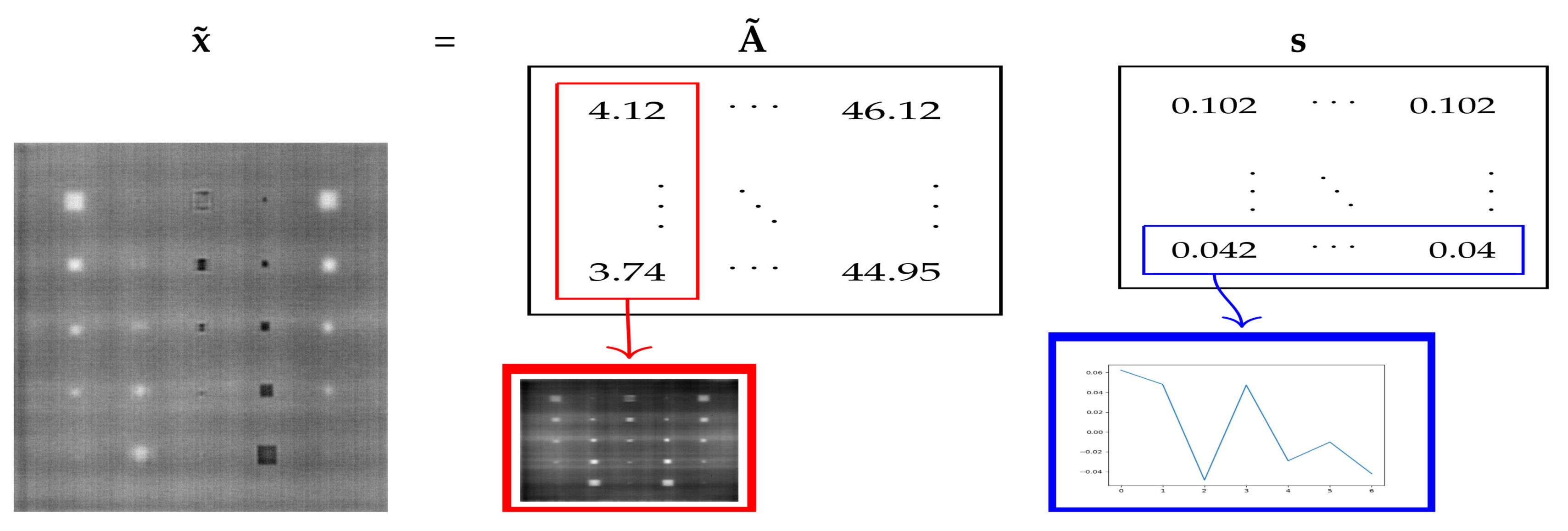
Figure 1. Illustation of the ICA Equation.
Applsci 11 04377 g001
Figure 2. CFRP sample used for the experiments.
Applsci 11 04377 g002
Figure 3. (a) CFRP plate; Z is the defect depth and labels are used to identify the location of each defect; (b) Pulsed thermography setup. a—PC, b—IR camera, c1 and c2—left and right flashes, and d—CFRP specimen.
Applsci 11 04377 g003
Figure 4. The blue contour represents the defect region, while the region between the green an red contours is our sound area.
Applsci 11 04377 g004
Figure 5. Research block diagram.
Applsci 11 04377 g005
Figure 6. Segmentation and accuracy computation flow diagram.
Applsci 11 04377 g006
Figure 7. Transformation of acquisition from a third-order tensor to a matrix.
Applsci 11 04377 g007
Figure 8. (a) represents an object ground truth. i.e., the white pixels represents an object. (b) represents the result of a segmentation algorithm. (c) represents the False Positive (FP) pixels of (b), i.e., the pixels that are labeled as part of an object but are not part of it. (d) represents the False Negative (FN) pixels of (b), i.e., the pixels that are labeled as not part of an object but are part of it. (e) represents the True Positive (TP) pixels of (b), i.e., the pixels that are properly labeled as part of an object. (f) represents the True Negative (TN) pixels of (b), i.e., the pixels that are properly labeled as not part of an object. Note that in figure (f) the black contour is a contour which is also present in all the figures.
Applsci 11 04377 g008
Figure 9. Maximum CNR score computed by defect depth as a function of the lateral size for all methods at frequency of 120 Hz and 145 Hz.
Applsci 11 04377 g009
Figure 10. Maximum CNR score computed by defect lateral size as a function of the depth for all methods at frequency of 120 Hz and 145 Hz.
Applsci 11 04377 g010
Figure 11. Comparative results between processing 7 and 100 components.
Applsci 11 04377 g011
Figure 12. Result of the computation of the IQR for each pixel of the mean sequence of 100 components and 7 components.
Applsci 11 04377 g012
Figure 13. Time of execution of the different methods.
Applsci 11 04377 g013
Figure 14. Results of the IQR for the differents ICA and state of the art algorithms.
Applsci 11 04377 g014
Figure 15. Results of the segmentation for the differents ICA and state of the art algorithms.
Applsci 11 04377 g015
Table 1. Comparison of PCA and ICA.
Features/MethodICAPCA
Linear transform
Goal of the transformationmaximizing the unmixing matrix as well as the independence of the components [10]project the data into an orthogonal space while maximizing the variance of the projected data [122]
Matrix factorizationfull rank to ensure the independence of the components.low rank to ensure the non-correlation of the components.
Othrogonalizenot by default, however commonly a whitening step is computed beforethe ICA, which othogonalize the data.
Ignore local data structure✓[28,41]
Denoise
Remove uneven heating
Table 2. Maximum CNR values for the different defects, for each method at the frequency of 120 and 145 Hz.
MethodDepth (mm)Lateral Size (mm)145 Hz vs. 120 HzLateral Size (mm)145 Hz vs. 120 HzLateral Size (mm)145 Hz vs. 120 HzLateral Size (mm)145 Hz vs. 120 HzLateral Size (mm)145 Hz vs. 120 Hz
3571015
120 Hz145 Hz120 Hz145 Hz120 Hz145 Hz120 Hz145 Hz120 Hz145 Hz
PCT0.23.7182.917−22%10.7116.456−40%12.40211.938−4%17.32316.317-6%8.69911.54433 %
0.41.5823.525123%9.7716.429−34%3.8628.991133%8.51210.48323%10.44816.44357%
0.62.7622.481−10%6.8987.63911%7.6177.8853%8.0307.273−9%8.69712.41743%
0.82.2441.608−28%4.1354.64912%6.1163.253−47%8.2409.11811%6.23610.44867%
10.6731.972193%3.0083.2538%4.1473.892−6%6.2347.44319%6.1636.2341%
PPT0.22.0752.94242%5.6975.450−4%7.0938.51720%8.1179.97523%4.9957.37848 %
0.41.3603.190134%7.2207.3101%3.97410.177156%7.4049.87933%7.87513.23868%
0.62.3082.288−0.89%6.7647.53311%6.5307.75719%7.2677.8067%7.06711.01556%
0.81.8801.276−32%3.9124.96427%5.5363.081−44%7.7377.528−3%5.8848.64947%
10.2170.791264%2.2393.08138%3.1883.71817%5.4146.39418%5.6716.95323%
Fast-ICA0.23.4742.802−19%12.8407.261−43%10.25912.07818%22.18416.903−24%12.98311.848−9%
0.41.5762.89984%6.7215.813−13%2.94010.698264%9.07710.29613%8.63212.48645%
0.61.7662.11520%4.3207.65277%4.8578.05066%4.3597.80079%3.50710.965213%
0.81.1121.44330%3.1654.73650%5.1453.333−35%6.2199.42151%4.87110.856123%
10.5741.461154%2.7943.33319%4.0863.853−6%5.6016.52216%5.7236.0766%
Infomax-ICA0.23.1662.823−11%9.5576.113−36%9.54811.27618%15.10114.707−3%10.24911.53512 %
0.41.6333.323103%9.1276.140−33%3.52010.247191%7.4248.0689%7.96015.11390%
0.63.0472.721−11%7.1838.28515%7.0398.14216%7.7337.553−2%8.68612.87848%
0.81.8371.775−3%3.9884.61716%5.3483.619−32%7.5249.23023%6.42411.47579%
10.8961.76797%2.2423.61961%3.4884.24221%5.1647.91753 %5.3387.47240%
Trust-region-ICA0.23.1522.840−10%9.7336.431−34%8.69012.60245%14.68915.7797%10.31011.46511%
0.41.3573.438153%8.4786.323−25%3.7508.390124%7.5817.8423%8.08015.11987%
0.62.5472.85912%6.4998.40829%6.5648.19125%7.4987.414−1%8.07213.16163%
0.81.8881.782−6%3.7464.42318%5.1243.628−29%7.4649.46227%5.95910.91983%
10.9262.000116%2.2393.62862%3.3364.49135%5.0469.01979%5.1647.93854%
Quasi-newton-ICA0.23.2262.897−10%9.9196.441−35%9.00213.20847%16.47815.678−5%10.50511.54010%
0.41.3253.217143%7.7256.056−22%3.4099.971192%6.7077.77116%7.46614.06388%
0.62.4462.6719%6.3308.29531%6.5138.24827%6.8467.60511%7.74312.62163%
0.81.8871.788−5%3.5134.69333%5.4643.645−33%6.9569.41335%5.72211.522101%
10.9391.85397%2.3073.64558%3.3534.29528%4.4777.74773%4.6517.33558 %
PICARD0.23.1662.820−11%9.5346.141−35%9.61211.36118%15.12014.846−2%10.24911.51412 %
0.41.6363.296101%9.1346.117−33%3.5259.539171%7.4288.0198%7.94814.90787%
0.63.0572.711−11%7.1958.28815%7.0568.15916%7.7577.577−2%8.67912.82048%
0.81.8471.778−4%4.0034.64116%5.3603.622−32%7.5229.27723%6.42911.52679%
10.8881.817104%2.2673.62260%3.4834.36725%5.1507.84152%5.3497.45439%
PICARD-O0.23.1632.818−11%9.6296.150−36%9.61211.39718%15.55114.899−4%10.30511.49511 %
0.41.6403.293101%9.1636.114−33%3.5189.378166%7.4527.9717%7.98314.76185%
0.63.0482.701−11%7.1698.28515%7.0228.16516%7.7367.568−2%8.69212.77647%
0.81.9231.764−8%3.9814.62816%5.5083.625−34%7.4899.27624%6.41811.47779%
10.8851.822106%2.3233.62556%3.6184.35820%5.1407.87353%5.3097.42540%
Table 3. Execution time of all methods.
MethodExecution Time (s)100 Comp. vs. 7 Comp.Execution Time (s)100 Comp. vs. 7 Comp.
FrequencyFrequency
120145
7 Comp.100 Comp.7 Comp.100 Comp.
Trust region ICA2.845139.086013.743.387239.596611.69
PICARD-O ICA59.9245134.36242.2463.8037134.70532.11
PICARD72.7453175.53882.4176.3144179.12372.35
Fast ICA38.155044.54241.1742.650746.52271.09
Infomax ICA5.041066.071113.115.459671.866013.16
Quasi newton ICA2.89807.36082.543.72717.56122.03
PCT8.756517.58892.09.250918.76922.02
Table 4. Accuracy score of different ICA methods segmentation.
MethodAccuracy Score
Frequency (Hz)
120145
PCT0.73100.8333
Trust region ICA0.93400.767
PICARD-O0.12700.6619
PICARD0.43970.7959
Fast ICA0.73190.8915
Infomax ICA0.22790.4832
Quasi newton ICA0.37580.7589
Publisher’s Note: MDPI stays neutral with regard to jurisdictional claims in published maps and institutional affiliations.