Distracted and Drowsy Driving Modeling Using Deep Physiological Representations and Multitask Learning
Abstract
1. Introduction
- Which physiological indicators are most indicative of drowsy and distracted behavior?
- Are there specific statistical features coming from different signals that are particularly informative?
- Is it possible to jointly tackle the problems of drowsiness and distraction detection and how such a framework can be formulated?
2. Related Work
2.1. Understanding Distracted and Drowsy Driving Using Physiological Signals
2.2. Deep Learning and Physiological Signal Processing for Driver State Modeling
2.3. Joint Learning of Multiple Driver Behaviors
3. Dataset and Experimental Setup
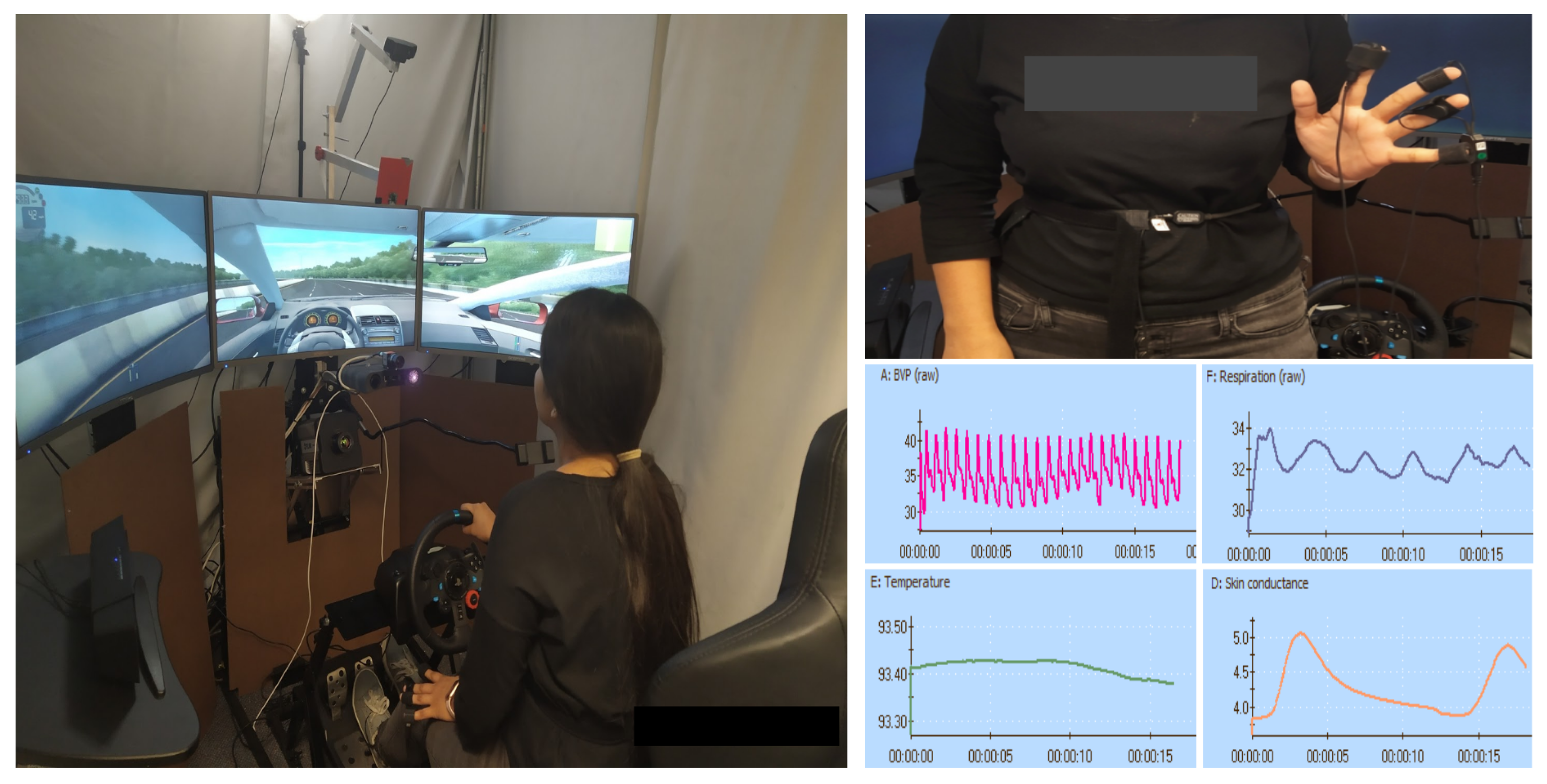
3.1. Experimental Procedure
- Texting—Physical. Participants were asked to type a small text message on their personal mobile device. The text was a predefined 8-word message and was dictated to the participant by the experiment supervisor on the fly. By using predefined texts we aimed to minimize the impact of cognitive effort that subjects had to put when texting and focus more on the physical disengagement from driving. Nonetheless, texting combines all three distraction classes defined by NHTSA and the CDC, which are Manual, Visual and Cognitive. The mobile device was placed on an adjustable holder on the right side of the steering wheel and participants had the freedom to adjust the positioning of the holder at will, so that it fits their personal preferences. Thus, simulating a real-car setup as accurately as possible.
- N-Back Test—Cognitive Neutral. The second distractor was the N-Back test. This distractor aimed to challenge exclusively the Cognitive capabilities of the subjects while driving. N-Back is a cognitive task extensively applied in psychology and cognitive neuroscience, designed to measure working memory [39]. For this distractor, participants were presented with a sequence of letters, and were asked to indicate when the current letter matched the one from n steps earlier in the sequence. For our experiments we set N = 1 and deployed an auditory version of the task where subjects had to listen to a prerecorded sequence of 50 letters.
- Listening to the Radio—Cognitive Emotional. For this distractor, participants were asked to listen to a pre-recorded audio from the news and then comment about what they just heard by expressing their personal thoughts. As with the N-Back Test, this distractor challenges mainly the cognitive capabilities of the participant when driving but with one major difference. In contrast to the neutral nature of the previous distractor here the recordings were emotionally provocative hence, motivating an affective response from the side of the subject. In particular, the two recordings used as stimuli for this part were related to a) a potential active shooter event that took place in the greater Detroit area and b) reporting from a fatal road accident scene which took place in the area of Chicago. These choices were made to help the users relate better to the events described in the recordings.
- GPS Interaction—Cognitive Frustration. At this step, we asked participants to find a specific destination on a ’GPS’ through verbal interaction. The goal of this distractor was to induce confusion and frustration to the participant; emotions that people are likely to experience when driving, either by interacting with similar ‘smart’ systems or through the engagement with other passengers or drivers on the road. In this case the ‘GPS’ was operated by a member of the research stuff in the background providing miss-leading answers to the participant and repeating mostly useless information until the desired answer was provided.
3.2. Modality Description
- Blood volume pulse (BVP): BVP is an estimate of heart rate based on the volume of blood that passes through the tissues in a localized area with each beat (pulse) of the heart. The BVP sensor shines infrared light through the finger and measures the amount of light reflected by the skin. The amount of reflected light varies during each heart beat as more or less blood rushes through the capillaries. The sensor converts the reflected light into an electrical signal that is then sent to the computer to be processed. BVB has been extensively used as an indicator of psychological arousal and is widely used as a method of measuring heart rate [40,41]. The BVP sensor was placed on the index finger. We collect BVP at a rate of 2048 Hz.
- Skin conductance: Skin conductance is collected by applying a low, undetectable and constant voltage to the skin and then measuring how the skin conductance varies. Similar to BVP, skin conductance variations are known to be associated with emotional arousal and changes in the signals produced by the sympathetic nervous system [41,42]. The sensor for these measurements was placed on the middle and ring fingers. Skin conductance signal is captured at 256 Hz.
- Skin temperature: This sensor measures temperature on the skin’s surface and captures temperatures between 10 C and 45 C (50 F–115 F). The temperature sensor was placed on the pinky finger. Skin temperature is also captured at 256 Hz.
- Respiration: The respiration sensor detects breathing by monitoring the expansion and contraction of the rib cage during inhalation and exhalation. By processing the captured periodic signal important characteristics can be computed such as respiration period, rate and amplitude. The respiration stripe was wrapped around the participant’s abdomen and the sensor was placed in the center of the body. Respiration is captured at 256 Hz.
3.3. Feature Extraction
- BVP features: Time domain statistical features such as mean, minimum, maximum and standard deviation are computed describing both the overall behavior of the signal but also the relation between consecutive inter-beat interval (IBI). NN related features describe the interval between two normal heartbeats. pNN features refer to the total number of pairs of consecutive normalized IBI values that differ more than 50 ms [43]. Additional features are computed to describe the spectral power statistics of different frequency bands by grouping the frequencies into three frequency bands, very-low (<0.04 Hz), low (0.04–0.15Hz) and high frequencies (0.15–0.4 Hz). For each frequency band, power related statistics are calculated.
- Respiration features: Amplitude, period and respiration rate are calculated along with the standard statistics from the raw respiration signal.
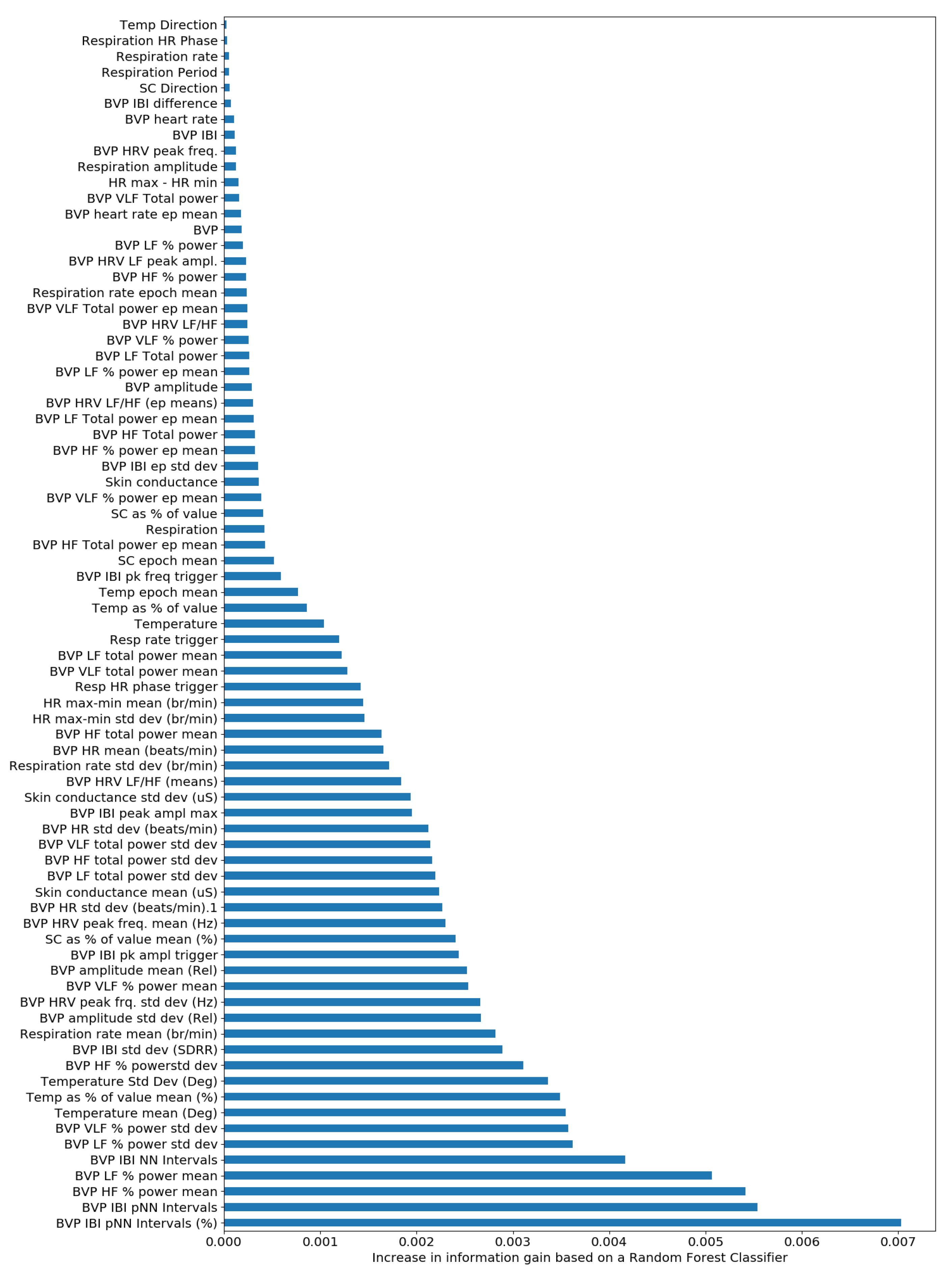
- Respiration + BVB features: Four features are computed that combine BVP and respiration measurements towards describing the peak to through difference in heart rate that occurs during a full breath cycle (HR Max-Min features as seen in Figure A1 in the Appendix A).
- Skin conductance and skin temperature features: Six features are extracted from each signal describing standard temporal statistics over short and long term windows on top of the raw the measurements. Features include the measurement as a percentage of change, the long and short term window means, the standard deviation of the short term window, the direction/gradient of the signals and the measurement as a percentage of the mean in the short term window.
3.4. Feature Selection
3.5. Metrics and Evaluation
- Sensitivity: Sensitivity (or positive recall), is estimated as the proportion of positive samples that are classified correctly. In the context of this paper, sensitivity describes the percentage of drowsy or distracted samples that are being correctly identified. The formula to compute sensitivity in terms of true positives (TP) and false negatives (FN) is: .
- Specificity: Specificity (or negative recall) is estimated as the proportion of negative samples that are classified correctly. In the context of this paper, specificity describes the percentage of alert or not-distracted samples that are being correctly identified. The formula to compute sensitivity in terms of true negatives (TN) and false positives (FP) is: .
- Average recall: Average recall corresponds to the mean value between specificity and sensitivity. The higher the average recall the less severe the trade-off between sensitivity and specificity.
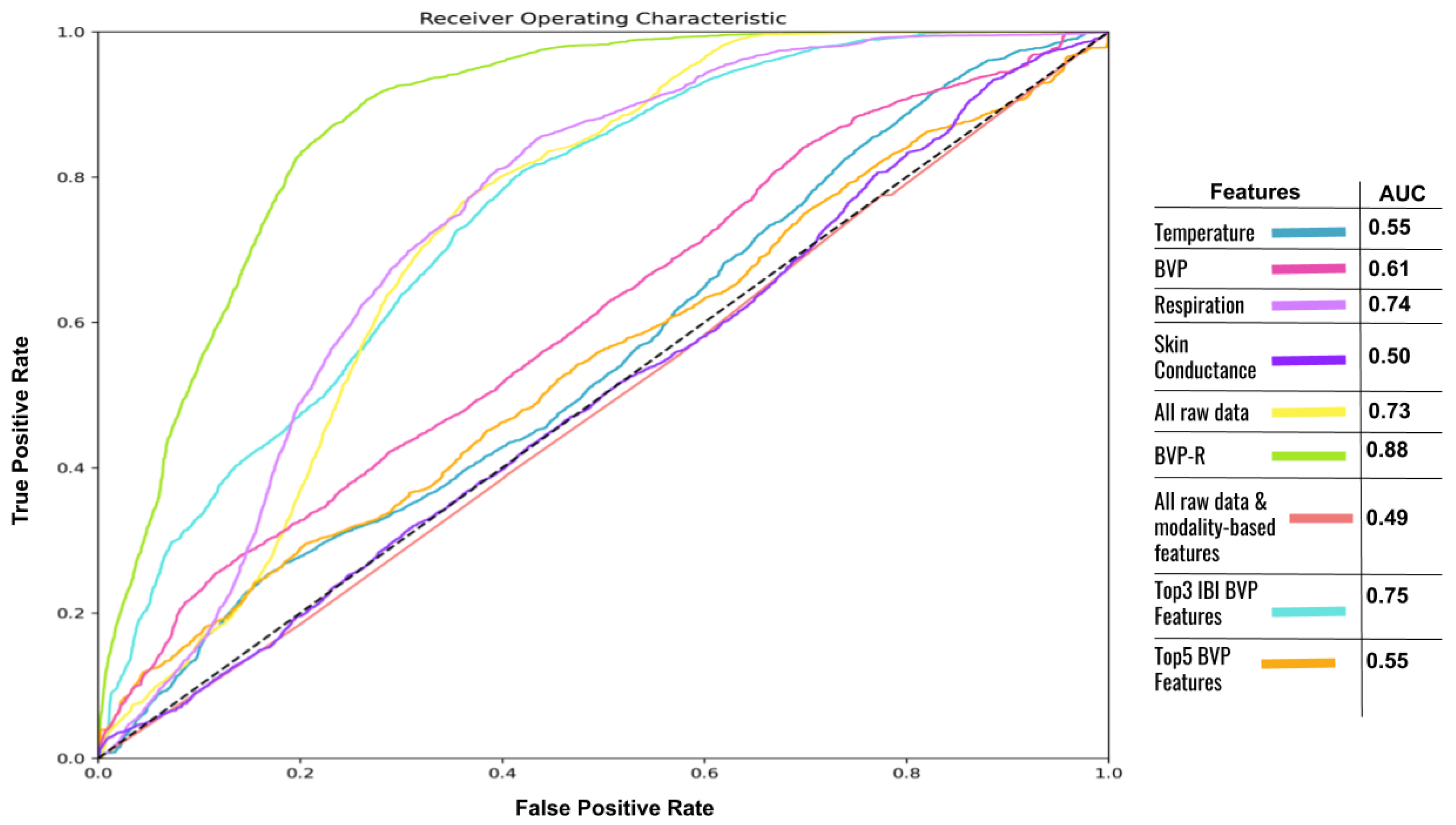
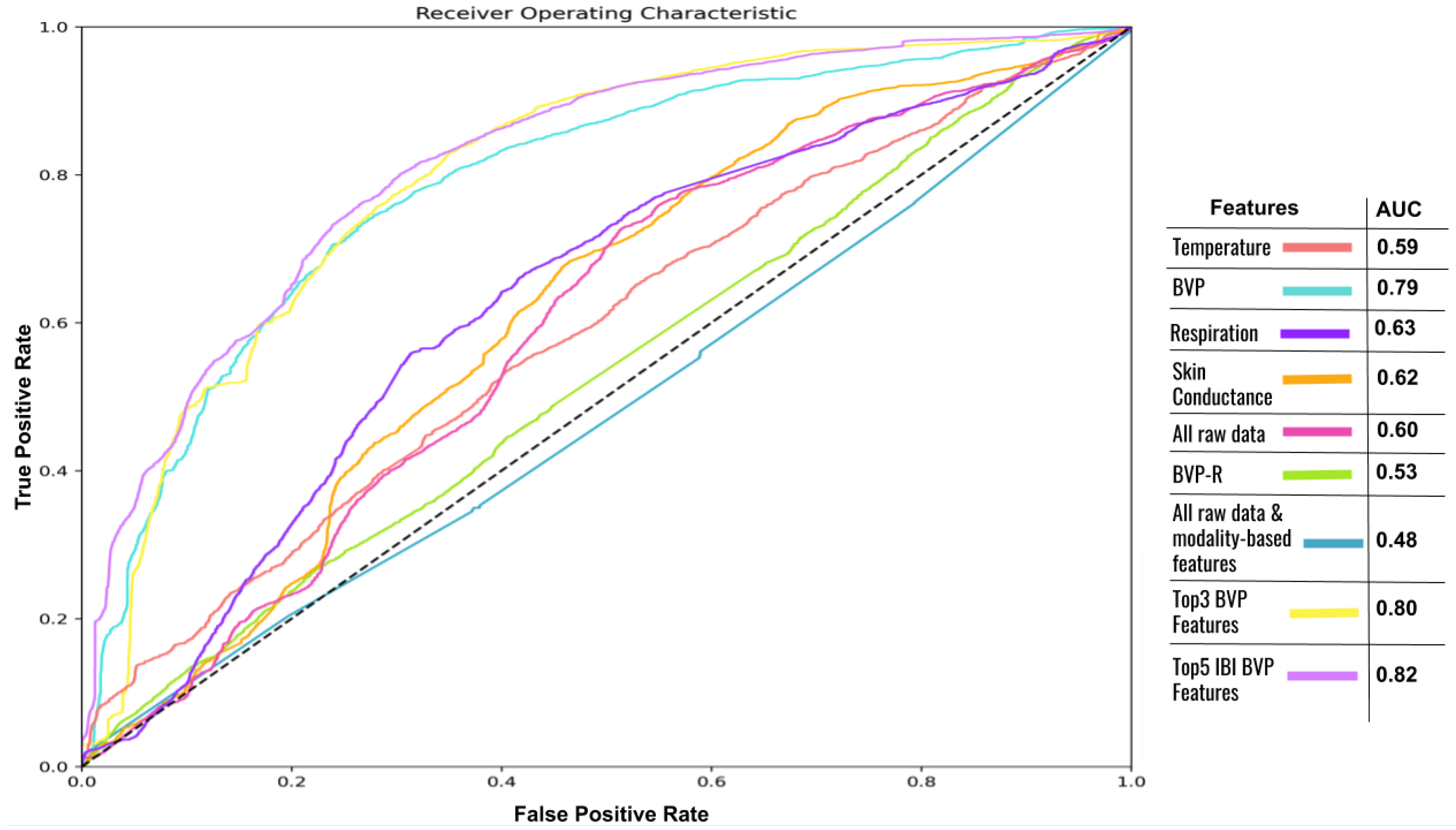
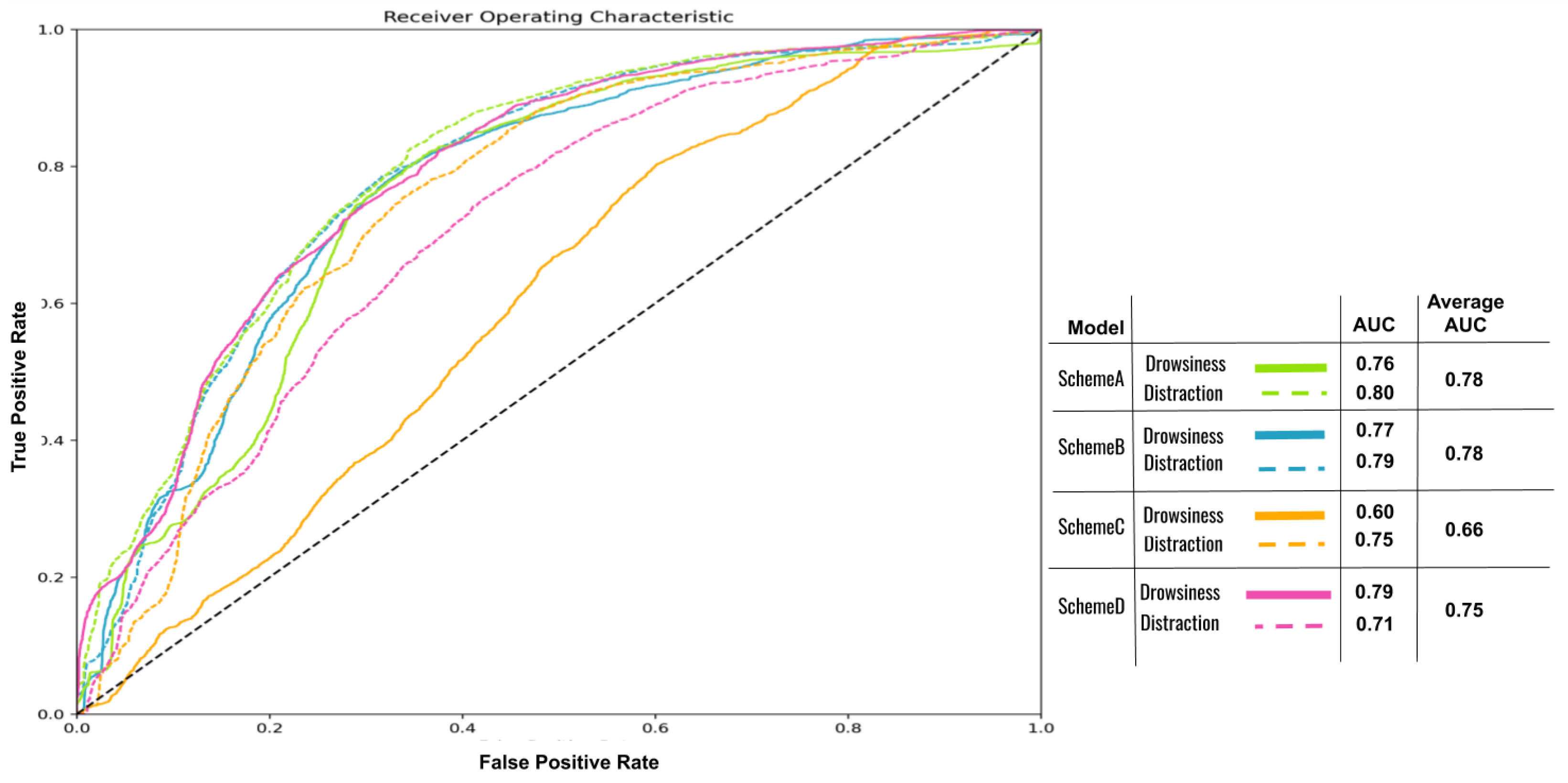
- Receiver operating characteristic curve (ROC): ROC curve is a graphical way to visualize the classification ability of a binary classifier. ROC curves describe the relation between TP-rate and FP-rate at different thresholds. FP-rate is given as 1-specificity. The area under the ROC curve is equal to the probability that the model will classify a randomly chosen positive instance higher than a randomly chosen negative one. The area under the ROC curve, also known as AUC, is a measure of the general ability of the network to discriminate between the two classes. The higher the AUC, the better the model.
3.6. Normalization and Classification Setup
4. Single and Joint Task Learning
4.1. Single Task Learning
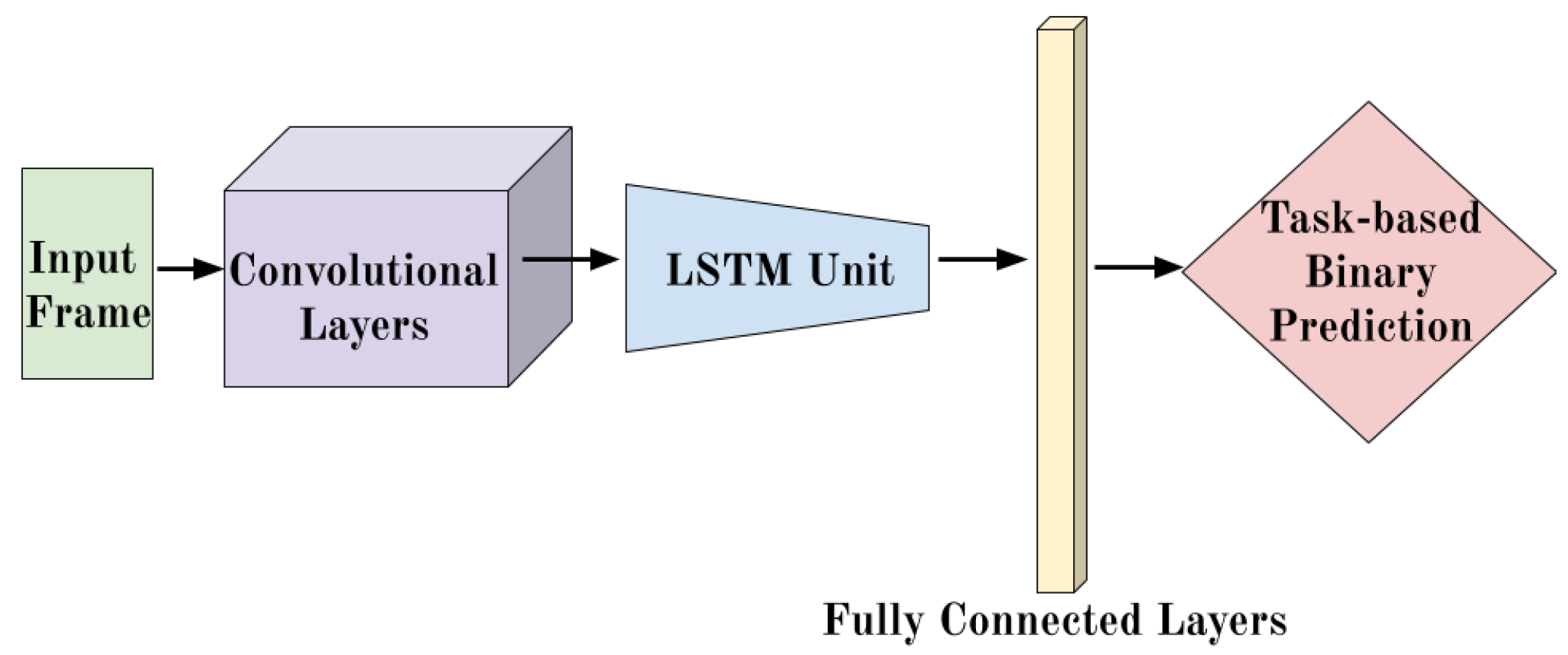
- A CNN-LSTM pipeline. The evaluated deep architecture was initially proposed by Donahue et al. in 2015 for video captioning and since then has been evaluated on several tasks that are based on physiological signal monitoring [53,54] mostly related to the medical domain. Only quite recently was the method also applied for the problem of multimodal stress monitoring in drivers [30]. The general model structure is shown in Figure 2. Our model, consists of two convolutional layers with 64 filters of size five, followed by an LSTM unit with a memory of 64. At the end, a fully connected layer of size 64 with a softmax activation for classification is applied. After each convolutional layer a 20% dropout is performed. The model is optimized based on categorical cross-entropy using an Adam optimizer [55]. All the hyper-parameters of the model, including the number and size of the different layers, were tuned after experimentation and through an exhaustive grid search evaluation of different parameter-value combinations. The proposed method performs practically two levels of temporal modeling on the input data. First, the CNN takes as input windows of 64 corresponding to data captured over a period of 8 s. Then, the LSTM unit accounts for the sequence of incoming frames taking into account data captured over approximately the past 8.5 min (given that it has a memory of 64). This design provides the model with great temporal depth that allows it to better account for future changes in behavior.
4.2. Joint-Task Learning
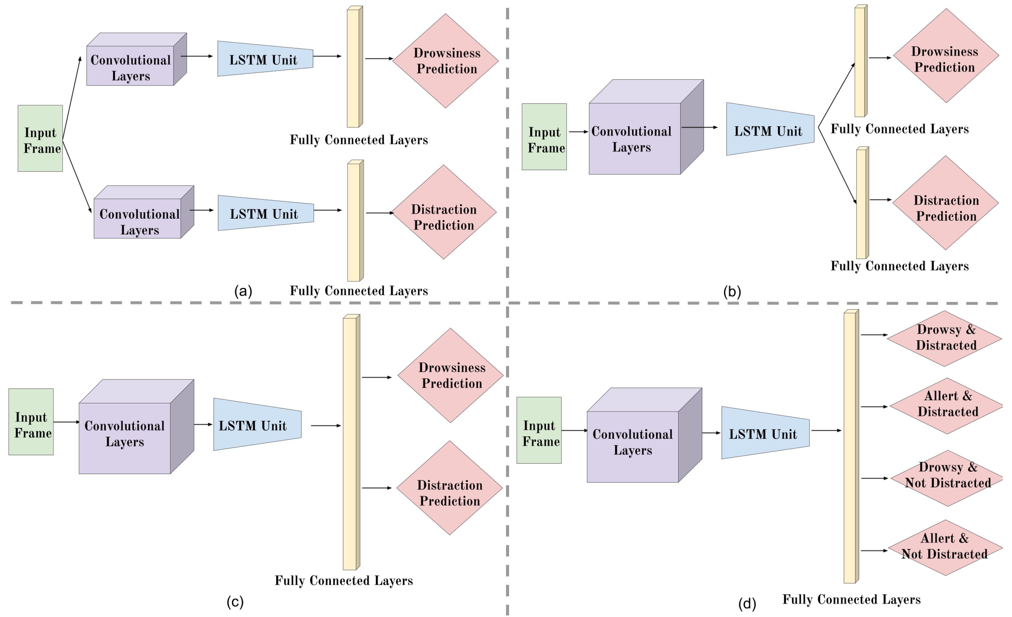
- Scheme A—Figure 3a: This model consists of two parallel networks, where each branch is dedicated to a specific task. Both branches are copies of the network shown in Figure 3. No layers are shared across the two tasks, but the two branches are trained using the same optimization function, which is estimated as the sum of task-based cross entropies. For getting a classification probability for each task a softmax function is applied at the dense layer of each branch.
- Scheme B—Figure 3b: This approach also formulates the problem as a multitask learning process. The difference compared to Scheme A is that both the convolutional and the LSTM layers are shared across the two tasks. After the LSTM unit, the network splits again into two branches with a dense layer dedicated explicitly on an individual task. As before the two tasks are optimized based on the average task-based cross entropies and a softmax function is used to estimate the probability of the assigned label at each branch.
- Scheme C—Figure 3c: In this approach we train a single network on a multilabel classification task. All layers are shared and a vector of size two is being predicted at the end, where each element corresponds to a task-specific label. The predicted vector values are estimated based on two sigmoid functions, each one dedicated to a specific task. In this case, all layers are shared across the two tasks and no task-based tailoring is being applied.
- Scheme D—Figure 3d: The last model formulates the problem as a single task multi-class classification process. In this case we have four labels, where each of them describes a unique combination of distracted and drowsy states. In particularly the four labels are: drowsy and distracted, drowsy and not-distracted, alert and distracted and alert and not-distracted. This formulation was inspired by the approach initially proposed by Riani et al. [26] where the authors did the same thing using a DT classifier.
5. Results
5.1. Single-Task Learning
- BVP: Raw BVP data plus 49 temporal features extracted from the BVP signal.
- Respiration: Raw respiration data plus eight temporal features extracted from the respiration signal.
- Skin conductance: Raw skin conductance data plus six temporal features extracted from the skin conductance signal.
- Temperature: Raw skin temperature data plus six temporal features extracted from the skin temperature signal.
- All raw data and modality-based features: The input data consist of the concatenation of all features and raw signals mentioned above.
- All raw data: Only the raw data from the four physiological sources are concatenated and used as input features.
- BVP + respiration (BVP-R): We evaluated different combinations of raw data as input features. Out of all the possible mixtures, combining BVP and respiration data stood out as the most efficient combination for part of our experiments.
- Top #5 BVP features: The input data consist of the top #5 (Table 2) performing features as identified through the analysis discussed in Section 3.4.
- Top #3 IBI BVP features: The input data consist of the top #3 BVP features that are related to IBI (features #1, #2 and #5 of Table 2).
5.2. Drowsy Driver Modeling
5.3. Distracted Driver Modeling
5.4. Multitask Learning for Joint Driving Behavior Modeling
6. Conclusions
- Which physiological indicators are most indicative of drowsy and distracted behavior?
- Are there specific statistical features coming from different signals that are particularly informative?
- Is it possible to jointly tackle the problems of drowsiness and distraction detection and how such a framework can be formulated?
Author Contributions
Funding
Institutional Review Board Statement
Informed Consent Statement
Data Availability Statement
Conflicts of Interest
Abbreviations
| AUC | area under curve |
| BPM | beats per minute |
| BR | breathing rate |
| BVP | blood volume pulse |
| CNN | convolutional neural network |
| DT | decision tree |
| FN | false negatives |
| FP | false positives |
| LSTM | long short-term memory |
| ECG | electrocardiogram |
| EEG | electroencephalogram |
| EMG | electromyogram |
| GSR | galvanic skin response |
| IBI | inter-beat intervals |
| KNN | K nearest neighbors |
| RF | random forest |
| ROC | receiver operating characteristic |
| SVM | support vector machine |
| TN | true negatives |
| TP | true positives |
| WHO | World Health Organization |
Appendix A
References
- Wang, Y.; Zhang, D.; Liu, Y.; Dai, B.; Lee, L.H. Enhancing transportation systems via deep learning: A survey. Transportation Research Part C: Emerging Technologies. 2019, 99, 144–163. [Google Scholar] [CrossRef]
- World Health Organisation. Mobile Phone Use: A Growing Problem Of Driver Distraction. 2011. Available online: https://www.who.int/violence_injury_prevention/publications/road_traffic/distracted_driving_en.pdf?ua=1 (accessed on 19 October 2020).
- World Health Organisation. Road Traffic Injuries. 2020. Available online: https://www.who.int/news-room/fact-sheets/detail/road-traffic-injuries (accessed on 19 October 2020).
- National Highway Traffic Safety Administration (NHTSA), US Department of Transportation. 2019; Distracted Driving. Available online: https://www.nhtsa.gov/risky-driving/distracted-driving (accessed on 19 October 2020).
- National Highway Traffic Safety Administration (NHTSA), US Department of Transportation. 2018; Drowsy Driving. Available online: https://www.nhtsa.gov/risky-driving/drowsy-driving (accessed on 19 October 2020).
- Sigari, M.H.; Fathy, M.; Soryani, M. A driver face monitoring system for fatigue and distraction detection. Int. J. Veh. Technol. 2013, 5, 73–100. [Google Scholar] [CrossRef]
- Kutila, M.; Jokela, M.; Markkula, G.; Rué, M.R. Driver distraction detection with a camera vision system. In Proceedings of the 2007 IEEE International Conference on Image Processing, San Antonio, TX, USA, 16–19 September 2007; IEEE: Piscataway, NJ, USA, 2007; Voume 6, p. VI-201. [Google Scholar]
- Yang, D.; Li, X.; Dai, X.; Zhang, R.; Qi, L.; Zhang, W.; Jiang, Z. All In One Network for Driver Attention Monitoring. In Proceedings of the ICASSP 2020-2020 IEEE International Conference on Acoustics, Speech and Signal Processing (ICASSP), Barcelona, Spain, 4–8 May 2020; IEEE: Piscataway, NJ, USA, 2020; pp. 2258–2262. [Google Scholar]
- Harbluk, J.L.; Noy, Y.I.; Trbovich, P.L.; Eizenman, M. An on-road assessment of cognitive distraction: Impacts on drivers’ visual behavior and braking performance. Accid. Anal. Prev. 2007, 39, 372–379. [Google Scholar] [CrossRef]
- Savelonas, M.; Karkanis, S.; Spyrou, E. Classification of Driving Behaviour using Short-term and Long-term Summaries of Sensor Data. In Proceedings of the 2020 5th South-East Europe Design Automation, Computer Engineering, Computer Networks and Social Media Conference (SEEDA-CECNSM), Corfu, Greece, 25–27 September 2020; IEEE: Piscataway, NJ, USA, 2020; pp. 1–4. [Google Scholar]
- Xie, Y.; Murphey, Y.L.; Kochhar, D. Personalized Driver Workload Estimation Using Deep Neural Network Learning from Physiological and Vehicle Signals. IEEE Trans. Intell. Veh. 2019. [Google Scholar] [CrossRef]
- Healey, J.A.; Picard, R.W. Detecting stress during real-world driving tasks using physiological sensors. IEEE Trans. Intell. Transp. Syst. 2005, 6, 156–166. [Google Scholar] [CrossRef]
- Singh, R.R.; Conjeti, S.; Banerjee, R. A comparative evaluation of neural network classifiers for stress level analysis of automotive drivers using physiological signals. Biomed. Signal Process. Control 2013, 8, 740–754. [Google Scholar] [CrossRef]
- Wang, K.; Guo, P. An Ensemble Classification Model With Unsupervised Representation Learning for Driving Stress Recognition Using Physiological Signals. IEEE Trans. Intell. Transp. Syst. 2020. [Google Scholar] [CrossRef]
- Desmond, P.A.; Matthews, G. Individual differences in stress and fatigue in two field studies of driving. Transp. Res. Part F Traffic Psychol. Behav. 2009, 12, 265–276. [Google Scholar] [CrossRef]
- Brookhuis, K.A.; De Waard, D. Monitoring drivers’ mental workload in driving simulators using physiological measures. Accid. Anal. Prev. 2010, 42, 898–903. [Google Scholar] [CrossRef]
- Reimer, B.; Mehler, B. The impact of cognitive workload on physiological arousal in young adult drivers: A field study and simulation validation. Ergonomics 2011, 54, 932–942. [Google Scholar] [CrossRef]
- Zhang, L.; Wade, J.; Bian, D.; Fan, J.; Swanson, A.; Weitlauf, A.; Warren, Z.; Sarkar, N. Cognitive load measurement in a virtual reality-based driving system for autism intervention. IEEE Trans. Affect. Comput. 2017, 8, 176–189. [Google Scholar] [CrossRef] [PubMed]
- Nourbakhsh, N.; Chen, F.; Wang, Y.; Calvo, R.A. Detecting users’ cognitive load by galvanic skin response with affective interference. ACM Trans. Interact. Intell. Syst. TiiS 2017, 7, 1–20. [Google Scholar] [CrossRef]
- Schmidt, M.; Bhandare, O.; Prabhune, A.; minker, W.; Werner, S. Classifying Cognitive Load for a Proactive In-car Voice Assistant. In Proceedings of the 2020 IEEE Sixth International Conference on Big Data Computing Service and Applications (BigDataService), Oxford, UK, 3–6 August 2020; IEEE: Piscataway, NJ, USA, 2020; pp. 9–16. [Google Scholar]
- Awais, M.; Badruddin, N.; Drieberg, M. A hybrid approach to detect driver drowsiness utilizing physiological signals to improve system performance and wearability. Sensors 2017, 17, 1991. [Google Scholar] [CrossRef] [PubMed]
- Persson, A.; Jonasson, H.; Fredriksson, I.; Wiklund, U.; Ahlström, C. Heart Rate Variability for Driver Sleepiness Classification in Real Road Driving Conditions. In Proceedings of the 2019 41st Annual International Conference of the IEEE Engineering in Medicine and Biology Society (EMBC), Berlin, Germany, 23–27 July 2019; IEEE: Piscataway, NJ, USA, 2019; pp. 6537–6540. [Google Scholar]
- Sahayadhas, A.; Sundaraj, K.; Murugappan, M.; Palaniappan, R. A physiological measures-based method for detecting inattention in drivers using machine learning approach. Biocybern. Biomed. Eng. 2015, 35, 198–205. [Google Scholar] [CrossRef]
- Taherisadr, M.; Asnani, P.; Galster, S.; Dehzangi, O. ECG-based driver inattention identification during naturalistic driving using Mel-frequency cepstrum 2-D transform and convolutional neural networks. Smart Health 2018, 9, 50–61. [Google Scholar] [CrossRef]
- Dehzangi, O.; Sahu, V.; Rajendra, V.; Taherisadr, M. GSR-based distracted driving identification using discrete & continuous decomposition and wavelet packet transform. Smart Health 2019, 14, 100085. [Google Scholar]
- Riani, K.; Papakostas, M.; Kokash, H.; Abouelenien, M.; Burzo, M.; Mihalcea, R. Towards detecting levels of alertness in drivers using multiple modalities. In Proceedings of the 13th ACM International Conference on PErvasive Technologies Related to Assistive Environments, Corfu, Greece, June 2020; pp. 1–9. [Google Scholar]
- Lim, S.; Yang, J.H. Driver state estimation by convolutional neural network using multimodal sensor data. Electron. Lett. 2016, 52, 1495–1497. [Google Scholar] [CrossRef]
- Zeng, H.; Yang, C.; Dai, G.; Qin, F.; Zhang, J.; Kong, W. EEG classification of driver mental states by deep learning. Cogn. Neurodynamics 2018, 12, 597–606. [Google Scholar] [CrossRef]
- Choi, H.T.; Back, M.K.; Lee, K.C. Driver drowsiness detection based on multimodal using fusion of visual-feature and bio-signal. In Proceedings of the 2018 International Conference on Information and Communication Technology Convergence (ICTC), Jeju Island, Korea, 17–19 October 2018; IEEE: Piscataway, NJ, USA, 2018; pp. 1249–1251. [Google Scholar]
- Rastgoo, M.N.; Nakisa, B.; Maire, F.; Rakotonirainy, A.; Chandran, V. Automatic driver stress level classification using multimodal deep learning. Expert Syst. Appl. 2019, 138, 112793. [Google Scholar] [CrossRef]
- Gjoreski, M.; Gams, M.Ž.; Luštrek, M.; Genc, P.; Garbas, J.U.; Hassan, T. Machine Learning and End-to-End Deep Learning for Monitoring Driver Distractions From Physiological and Visual Signals. IEEE Access 2020, 8, 70590–70603. [Google Scholar] [CrossRef]
- Craye, C.; Rashwan, A.; Kamel, M.S.; Karray, F. A multi-modal driver fatigue and distraction assessment system. Int. J. Intell. Transp. Syst. Res. 2016, 14, 173–194. [Google Scholar] [CrossRef]
- Choi, M.; Koo, G.; Seo, M.; Kim, S.W. Wearable device-based system to monitor a driver’s stress, fatigue, and drowsiness. IEEE Trans. Instrum. Meas. 2017, 67, 634–645. [Google Scholar] [CrossRef]
- Sarkar, P.; Ross, K.; Ruberto, A.J.; Rodenbura, D.; Hungler, P.; Etemad, A. Classification of cognitive load and expertise for adaptive simulation using deep multitask learning. In Proceedings of the 2019 8th International Conference on Affective Computing and Intelligent Interaction (ACII), Cambridge, UK, 3–6 September 2019; IEEE: Piscataway, NJ, USA, 2019; pp. 1–7. [Google Scholar]
- National Heart, Lung, and Blood Institute and National Highway Traffic Safety Administration (NHTSA). Drowsy Driving and Automobile Crashes. 1998. Available online: https://rosap.ntl.bts.gov/view/dot/1661 (accessed on 7 December 2020).
- Beirness, D.J.; Herb, M.; Desmond, K. The road safety monitor 2004: Drowsy driving. In The 2004 Annual Public Opinion Survey by the Traffic Injury Research Foundation; Traffic Injury Research Foundation (TIRF): Ottowa, ON, Canada.
- Caponecchia, C.J.; Williamson, A. Drowsiness and driving performance on commuter trips. J. Saf. Res. 2018, 66, 179–186. [Google Scholar] [CrossRef] [PubMed]
- Guede, F.; Chimeno, M.; Castro, J.; Gonzalez, M. Driver drowsiness detection based on respiratory signal analysis. IEEE Access 2019, 7, 81826–81838. [Google Scholar] [CrossRef]
- Kane, M.J.; Conway, A.R.; Miura, T.K.; Colflesh, G.J. Working memory, attention control, and the N-back task: A question of construct validity. J. Exp. Psychol. Learn. Mem. Cogn. 2007, 33, 615. [Google Scholar] [CrossRef] [PubMed]
- Karthikeyan, P.; Murugappan, M.; Yaacob, S. Descriptive analysis of skin temperature variability of sympathetic nervous system activity in stress. J. Phys. Ther. Sci. 2012, 24, 1341–1344. [Google Scholar] [CrossRef]
- Mackersie, C.L.; Calderon-Moultrie, N. Autonomic nervous system reactivity during speech repetition tasks: Heart rate variability and skin conductance. Ear Hear. 2016, 37, 118S–125S. [Google Scholar] [CrossRef]
- Storm, H.; Myre, K.; Rostrup, M.; Stokland, O.; Lien, M.; Raeder, J. Skin conductance correlates with perioperative stress. Acta Anaesthesiol. Scand. 2002, 46, 887–895. [Google Scholar] [CrossRef]
- Malik, M.; Bigger, J.T.; Camm, A.J.; Kleiger, R.E.; Malliani, A.; Moss, A.J.; Schwartz, P.J. Heart rate variability: Standards of measurement, physiological interpretation, and clinical use. Eur. Heart J. 1996, 17, 354–381. [Google Scholar] [CrossRef]
- Hearst, M.A.; Dumais, S.T.; Osuna, E.; Platt, J.; Scholkopf, B. Support vector machines. IEEE Intell. Syst. Their Appl. 1998, 13, 18–28. [Google Scholar] [CrossRef]
- Li, G.; Chung, W.Y. Detection of driver drowsiness using wavelet analysis of heart rate variability and a support vector machine classifier. Sensors 2013, 13, 16494–16511. [Google Scholar] [CrossRef] [PubMed]
- Chen, H.; Chen, L. Support vector machine classification of drunk driving behaviour. Int. J. Environ. Res. Public Health 2017, 14, 108. [Google Scholar] [CrossRef] [PubMed]
- Yakowitz, S. Nearest-neighbour methods for time series analysis. J. Time Ser. Anal. 1987, 8, 235–247. [Google Scholar] [CrossRef]
- Munla, N.; Khalil, M.; Shahin, A.; Mourad, A. Driver stress level detection using HRV analysis. In Proceedings of the 2015 international conference on advances in biomedical engineering (ICABME), Beirut, Lebanon, 16–18 September 2015; IEEE: Piscataway, NJ, USA, 2015; pp. 61–64. [Google Scholar]
- Wang, J.S.; Lin, C.W.; Yang, Y.T.C. A k-nearest-neighbor classifier with heart rate variability feature-based transformation algorithm for driving stress recognition. Neurocomputing 2013, 116, 136–143. [Google Scholar] [CrossRef]
- Liaw, A.; Wiener, M. Classification and regression by randomForest. R News 2002, 2, 18–22. [Google Scholar]
- Hassib, M.; Braun, M.; Pfleging, B.; Alt, F. Detecting and influencing driver emotions using psycho-physiological sensors and ambient light. In IFIP Conference on Human-Computer Interaction; Springer: Berlin/Heidelberg, Germany, 2019; pp. 721–742. [Google Scholar]
- Wang, M.; Jeong, N.; Kim, K.; Choi, S.; Yang, S.; You, S.; Lee, J.; Suh, M. Drowsy behavior detection based on driving information. Int. J. Automot. Technol. 2016, 17, 165–173. [Google Scholar] [CrossRef]
- Faust, O.; Hagiwara, Y.; Hong, T.J.; Lih, O.S.; Acharya, U.R. Deep learning for healthcare applications based on physiological signals: A review. Comput. Methods Programs Biomed. 2018, 161, 1–13. [Google Scholar] [CrossRef]
- Rim, B.; Sung, N.J.; Min, S.; Hong, M. Deep Learning in Physiological Signal Data: A Survey. Sensors 2020, 20, 969. [Google Scholar] [CrossRef]
- Kingma, D.P.; Ba, J. Adam: A method for stochastic optimization. arXiv 2014, arXiv:1412.6980. [Google Scholar]
- Shahid, A.; Wilkinson, K.; Marcu, S.; Shapiro, C. Karolinska sleepiness scale (KSS). In STOP, THAT and One Hundred Other Sleep Scales; Springer: New York, NY, USA, 2011; pp. 209–210. [Google Scholar]
- Basner, M.; Mollicone, D.; Dinges, D. Validity and sensitivity of a brief psychomotor vigilance test (PVT-B) to total and partial sleep deprivation. Acta Astronaut. 2011, 69, 949–959. [Google Scholar] [CrossRef]
| Recording Segment | |||||
|---|---|---|---|---|---|
| Free-driving | Texting Physical | NBack Cognitive Neutral | Radio Cognitive Emotional | GPS Cognitive Frustration | |
| #Data (hours) | ∼7.4 | ∼3.1 | ∼2.2 | ∼3.4 | ∼2 |
| Feature | Description | |
|---|---|---|
| #1 | BVP IBI pNN Intervals (%) | the percentage of successive intervals that differ by more than 50 ms |
| #2 | BVP IBI pNN Intervals | the number of successive intervals that differ by more than 50 ms |
| #3 | BVP HF % power mean | the mean of power in the high frequencies |
| #4 | BVP LF % power mean | the mean of power in the low frequencies |
| #5 | BVP IBI NN Intervals | interval between two normal heartbeats |
| Drowsiness Detection | ||||
|---|---|---|---|---|
| SVM | KNN | RF | CNN-LSTM | |
| Sensitivity (%) | 0 | 17 | 17 | 93 |
| Specificity (%) | 92 | 91 | 91 | 71 |
| Average Recall (%) | 46 | 54 | 54 | 82 |
| Distraction Detection | ||||
|---|---|---|---|---|
| SVM | KNN | RF | CNN-LSTM | |
| Sensitivity (%) | 53 | 69 | 70 | 70 |
| Specificity (%) | 72 | 52 | 50 | 74 |
| Average Recall (%) | 62.5 | 60.5 | 60 | 72 |
| Joint Condition Learning | ||||||||
|---|---|---|---|---|---|---|---|---|
| SVM | KNN | RF | Scheme A | Scheme B | Scheme C | Scheme D | ||
| Drowsiness Detection | Sensitivity (%) | 45 | 25 | 24 | 77 | 73 | 82 | 69 |
| Specificity (%) | 64 | 78 | 91 | 68 | 72 | 37 | 63 | |
| Average Recall (%) | 54.5 | 51.5 | 57.5 | 72.5 | 72.5 | 59.5 | 66 | |
| Distraction Detection | Sensitivity (%) | 51 | 58 | 70 | 75 | 78 | 84 | 78 |
| Specificity (%) | 73 | 52 | 50 | 71 | 68 | 56 | 66 | |
| Average Recall (%) | 62 | 55 | 60 | 73 | 73 | 70 | 72 | |
Publisher’s Note: MDPI stays neutral with regard to jurisdictional claims in published maps and institutional affiliations. |
© 2020 by the authors. Licensee MDPI, Basel, Switzerland. This article is an open access article distributed under the terms and conditions of the Creative Commons Attribution (CC BY) license (http://creativecommons.org/licenses/by/4.0/).
Share and Cite
Papakostas, M.; Das, K.; Abouelenien, M.; Mihalcea, R.; Burzo, M. Distracted and Drowsy Driving Modeling Using Deep Physiological Representations and Multitask Learning. Appl. Sci. 2021, 11, 88. https://doi.org/10.3390/app11010088
Papakostas M, Das K, Abouelenien M, Mihalcea R, Burzo M. Distracted and Drowsy Driving Modeling Using Deep Physiological Representations and Multitask Learning. Applied Sciences. 2021; 11(1):88. https://doi.org/10.3390/app11010088
Chicago/Turabian StylePapakostas, Michalis, Kapotaksha Das, Mohamed Abouelenien, Rada Mihalcea, and Mihai Burzo. 2021. "Distracted and Drowsy Driving Modeling Using Deep Physiological Representations and Multitask Learning" Applied Sciences 11, no. 1: 88. https://doi.org/10.3390/app11010088
APA StylePapakostas, M., Das, K., Abouelenien, M., Mihalcea, R., & Burzo, M. (2021). Distracted and Drowsy Driving Modeling Using Deep Physiological Representations and Multitask Learning. Applied Sciences, 11(1), 88. https://doi.org/10.3390/app11010088


