More on Pipelined Dynamic Scheduling of Big Data Streams

Abstract

An important as well as challenging task in modern applications is the management and processing with very short delays of large data volumes. It is quite often, that the capabilities of individual machines are exceeded when trying to manage such large data volumes. In this regard, it is important to develop efficient task scheduling algorithms, which reduce the stream processing costs. What makes the situation more difficult is the fact that the applications as well as the processing systems are prone to changes during runtime: processing nodes may be down, temporarily or permanently, more resources may be needed by an application, and so on. Therefore, it is necessary to develop dynamic schedulers, which can effectively deal with these changes during runtime. In this work, we provide a fast and fair task migration policy while maintaining load balancing and low latency times. The experimental results have shown that our scheme offers better load balancing and reduces the overall latency compared to the state of the art strategies, due to the stepwise communication and the pipeline based processing it employs.

1. Introduction

The increasing availability of sensors and computing devices (from smaller to larger ones) has led to a tremendous increase in the data volumes being produced and imposed certain needs of some kind of data analysis. The rapid growth of cloud computing and Internet of Things (IoT) promoted the sharp growth of data further. Managing the produced data and gaining insights from it, is a big challenge. Many organizations’ decisions depend on the analysis and processing of this data, just as it arrives. Environmental monitoring, fraud detection, emergency response, sensors, scientific experiments are just a few examples of applications that require continuous and timely processing of information [1,2,3,4,5]. The term “big data” refers to these huge amounts of data and the challenges posed to its transfer, processing, storage, and use.

For most of the big data applications mentioned just above, the data have some value only in cases when they are analyzed at a time very close to the time they were actually produced. This means that the vast and continuous data streams should be scheduled in such a way, that they are delivered to the processing elements and be processed with very short delays. Therefore, an efficient plan to place specific processing tasks on specific processing resources and to control the job execution has to be employed. The careful arrangement of tasks into the cluster resources, so that the task completion time is minimized and resource utilization is achieved is known as scheduling and it is a very important factor in the overall processing of big data streams. Efficient task scheduling algorithms reduce the processing latencies and significantly improve resource utilization and the platform stability of cloud services. Therefore, these schedulers are absolutely necessary to deal with transmission of massive data among large-scale tasks.

The difficulty of the scheduling problem is aggravated by the dynamic nature of both the applications and the cloud environment on which they run. Particularly, challenges present themselves when the system parameters (like the number of available processing nodes or executing tasks) need to change during runtime. This is a quite natural scenario, considering the fact that an application may require more resources from the cloud whenever they are available or, in the reverse scenario, some processing or transferring resources may become temporarily unavailable while an application is running. Static schedulers cannot efficiently handle such cases [6,7]. Therefore, dynamic schedulers which can effectively deal with these changes during runtime are quite important to handle big data applications.

The dynamic scheduling strategies generally deal with the important and interrelated issues of task migrations (or state migrations) and of elasticity. Task migrations refer to the cases where some tasks have to be assigned to a node other than the one they are being executed. However, these tasks have to migrate along with their context or state (for example, all the data having been processed, assigned variable values, etc.). Thus, the overall latency can increase and this poses another big challenge for the scheduling strategies. The elasticity refers to the ability of a cloud system to allow an executing program to obtain additional resources or release idle resources as required. Some challenges regarding elasticity include the placement of processing tasks on available resources (processing nodes), the handling of node failures to which an application has to adapt properly, and the network contentions among transferred stream.

Apparently, the degree to which a system can handle system changes both in terms of resources and executing tasks is of vital importance. For example, the buffer space required for an application’s data may need to change, load balancing strategies need to be imposed as some nodes with very heavy processing load may become a bottleneck for the whole system, and tasks may need to migrate, for example in cases of node crushes. It is rather important to handle such cases in an efficient manner to maintain overall optimal performance of the system.

In this work, we extend our previous research efforts [1] in order to develop a scheme that can also redistribute the migrated tasks in a fair and fast way by examining the load of the nodes in close proximity to the node whose tasks are to be migrated. In this way, we manage to maintain the system’s load balancing and reduce the overall latency as our simulation results have shown. The main contributions of this work are the following:

• It uses our previously designed scheduler to handle task migrations as well. This feature was not present in our previous work.
• It introduces an straightforward model to estimate each node’s load, in order to decide about the task migrations.
• The total processing latencies can still be reduced by the pipeline based method we proposed in our previous scheme.
• This work is expandable to larger-scale networks.

In the remainder of this work, we initially describe some schemes that handle the elasticity and task migration issues. Then, in Section 3, we present some mathematical preliminaries and our communication scheduling policy. This section includes already published material which we present in a few pages to make the paper self-contained. In Section 4, we present the model that estimates the load assigned to each node in order to make a fair distribution of migrated tasks. In Section 5, we present our pipeline-based scheduling, which includes not only the data transferring and processing stages of every stream processing problem, but the task migrations as well. Section 6 presents our simulation results, where we compare our strategy in terms of load balancing and latency with two well known state-of-the-art schemes. Section 7 concludes this work and offers aspects for future work.

2. Related Work and Discussion

Generally, the change of parallelization degree (number of nodes working in parallel) of a stream processing system is the main reason that causes the necessity for state migrations. In such cases, the usual practice is to use some type of system monitoring, where a system monitor observes the usage of the system’s resources (links, CPU, memory) [5,8,9,10,11,12]. After monitoring, some type of strategy determines where the tasks are going to migrate. In this paragraph, we discuss papers that mostly focus their attention on migration policies.

In [13], the authors define five operator patterns based on which they generate rules for increasing scalability by load distribution and achieving elasticity: (1) Simple Standby: For a critical query node N there is a standby node S on a separate unit. This standby node is activated in case of failure of node N, so N needs to be continuously monitored. (2) Checkpointing: Similar to 1, but supports stateful operators for storing and accessing information across multiple events (stateless operators store and access information based on the last event only). The state of N is periodically monitored and the standby node S restarts from this checkpoint. (3) Hot Standby: The input stream is sent to redundant nodes S, usually by multicasting, so they act as hot standby’s whenever the time of failure incurred during checkpointing is unacceptable. This pattern works for stateful and stateless operators. (4) Stream Partitioning: The input stream is partitioned and each tuple is directed to one of the nodes $N_1,\cdots N_n$. This pattern is used to exploit data parallelization. and (5) Stream Pipelining: Same as pattern 4, but the streams are placed to different computation units to be processed in a pipeline fashion.

In [14], the authors manage and expose the operator state directly to the stream processing system. In this way, they create an integrated approach for dynamic scale out and recovery of the stateful operators. The operator state is periodically checkpointed by the stream processing engine and the state is backed-up. When possible bottlenecks are identified through monitoring of the CPU utilization, a scale-out operation is invoked and new virtual machines are allocated. The checkpointed state is re-partitioned and the overall processing is divided between the new processing elements. This scaling out increases parallelization when the system resource monitoring gives results which are above a predefined threshold. Recovery of failed operators is achieved by restoring the checkpointed state on a new virtual machine and replaying and unprocessed tuples.

Heinze et al. [15] propose an approach named FUGU, which optimizes the scaling policy automatically. Thus the user avoids the need to set the configuration parameters for a selected scaling policy. The idea is to use an online parameter optimization approach. The approach employs three algorithms: a Scaling Algorithm, that takes decisions that characterize a host as overloaded or underloaded, based on a vector of measurements regarding the node utilization (CPU, memory, and network elements), an Operator Selection algorithm, which decides which operators to move, and an Operator Placement algorithm, which determines where to move these operators.

Each scaling decision is translated into a set of moving operators. If the system is found to be underloaded, it selects all operators running on the least loaded hosts, in other words, it releases a host with minimum latencies (scale-in). When a host is found overloaded, the Operator Selection algorithm chooses a subset of operators to remain in the host, so that their summed load is smaller than the given threshold. The remaining operators will move to a new host (scale-out). The operator placement is modeled as a problem defined by nodes occupying a CPU capacity and by operators with a certain CPU load.

In [16], the authors introduce a model for estimating the latency of a data flow, when the level of parallelization between the tasks changes. They continuously measure the necessary performance metrics, like CPU utilization thresholds, the rate of processed tuples per operator, and the overall latency. Thus, appropriate scaling actions are determined during runtime and thus the elasticity is enhanced. The main goal of the strategy is to provide latency guarantees while the resource use is minimized, in cases where the resource provisioning is variable. The latency under heavy data flows is estimated by an estimating model and the resource consumption is minimized using an automated strategy which aims at adjusting the data parallelization during runtime. A bottleneck resolving technique is used to resolve bottlenecks through scaling out, giving way to the parallelization adjustment scheme for future use.

In [17], an elastic stream processing scheme named StreamCloud is presented. StreamCloud introduces a new parallelization technique which divides queries into subqueries. These subqueries are allocated to independent node sets, such that the total overhead is minimized. The number of sub-queries depends on the number of stateful operators included in the original query. Each sub-query includes one stateful operator and all the stateless operators that follow until the next stateful operator. The elasticity protocols being employed allow for effective resource adjustment according to the incoming processing load. A resource management architecture monitors the resource utilization and the load is balanced if the utilization exceeds certain limits or it is beyond certain limits. The load balancing enables the minimization of the computational resources. In addition, other actions to be taken are to release or add resources. The load balancing is implemented via a load-balancing operator.

In [18,19], the authors identify four fundamental properties for their migration protocol: (i) Gracefulness: the splitter and the replicas should never discard input streams, process out-of-order any tuples having the same key or generate duplicated results. (ii) Fluidness: the splitter should not wait for the migration to complete before re-distributing new incoming tuples to the replicas. (iii) Non-intrusiveness: the migration should involve only the replicas which exchange parts of their state. (iv) Fluentness: a replica waiting to get the state of an incoming key during migration must be able to process all the input tuples having other keys and for which the state can be used. Based on these properties and after a reconfiguration decision, a reconfiguration message is transmitted to the splitter with a new routing table. Upon receipt of the reconfiguration message, the splitter becomes aware of the keys that must be migrated and transmits to the proper replicas the set of migration messages.

Xu et al. [20] introduced T-Storm, which aims at reducing the inter-process and inter-node communication. The workload and the traffic are monitored during runtime and the future load is estimated using a machine learning prediction method. A schedule generator periodically reads the above information from the database, sorts the executors in a descending order of their traffic load, and assigns executors to slots. Executors from one topology are assigned in the same slot to reduce inter-process traffic. The total executors’ workload should not exceed worker’s capacity and the number of executors per slot is calculated with the help of a control parameter.

In [21], the authors present STream processing ELAsticity (Stela), a stream processing system that supports scale-out and scale-in operations on-demand manner. Stela optimizes post-scaling throughput and minimizes interruption to the ongoing computation while carrying out scaling. For scale-out operations, Stela first identifies operators that are congested based on their input and output rates. Then it computes the Expected Throughput Percentage (ETP) on an operator basis. Based on the topology, it captures the percentage of the application throughput directly impacted by an operator and provides more resources to a congested operator with higher ETP to improve the overall application throughput. Based on the new execution speed achieved, Stela selects the next operator and repeats the process.

For scale-in operations, Stela assumes that the user simply specifies the number of machines to be removed and chooses the most suitable machines for removal based on the ETPSum. The ETPSum for a machine is the sum of all ETP of instances of all operators that currently reside on the machine. This is an indicator of the machine’s contribution to the overall throughput. Thus, machines with lower ETPSum are preferred for removal during scale-in.

In [22], the authors propose two task migration approaches that allow a running streaming dataflow to migrate, without any loss of in-flight messages or their internal tasks states: (i) the Drain, Checkpoint, and Restore (DCR) policy pauses the source tasks’ execution and allows the in-flight messages to execute across the dataflow until completion, thus draining the dataflow without any loss of messages. (ii) The Capture, Checkpoint, and Resume (CCR) directly broadcasts checkpoint events from the source task to each task in the dataflow and processes only one event, that is, the event that a task may currently be executing. In this way, extra latencies that incur from incremental flows of checkpoint messages and their full processing are reduced.

Ding et al. [23] introduced a scheme that performs live, progressive migrations without resorting to expensive synchronization barriers. In addition, they introduced algorithms for finding the optimal task assignment for the migration. The main components of the proposed migration mechanism include a migration manager (MM), a retriever of operator states from remote nodes, a re-router for misrouted tuples, and a file server that serves operator states to remote retrievers. When a migration is triggered, the master node notifies all the workers. Upon receiving such a notification, a worker updates its local task assignment. Then, the worker restarts the executors whose assigned tasks have changed. Finally, they introduced an algorithm to maintain statistics from past workloads to predict future migration costs.

N-Storm [24] is a thread-level task migration scheme for Storm. N-Storm adds a key/value store on each worker node to make workers be aware of the changes of the overall task scheduling. In this regard, a worker node can manage its executors during run time (kill or start executors). With this mechanism, unnecessary stopping of executors and workers during a task migration is avoided and the performance of task migration is improved. Further they optimized N-Storm to make it efficient for multiple task migrations.

Cardellini et al. [25] modeled the elasticity problem for data stream processing as a linear programming problem, which is used to optimize different QoS metrics. For the operator migration, they proposed a general formulation of the reconfiguration costs and they considered that system performs the state migrations leveraging on a storage system, called DataStore which stores the operators code and allows replicas to save and restore their state when reconfigurations occur.

In addition, the work of Ma et al. [26] presented a migration cost model and a balance model as metrics to evaluate their migration strategy. Based on these models, a live data migration strategy with particle swarm optimization (PSO) was proposed, with two improvement measures, the loop context, and particle grouping. As an improvement of stream processing framework, the nested loop context structure supports the iterative optimization algorithm. Grouping particles before in-stream processing speeds up the convergence rate of the PSO policy.

A different, however interesting approach called E-Storm [27] is a replication-based state management that actively maintains multiple state backups on different nodes. A recovery module restores any lost states by transferring states among the tasks. In this way, lost task states are recovered in case of JVM or node crashes.

In [28], the authors presented a work on the placement and deployment of data stream processing applications in geo-distributed environments. The strategy targeted fog resources and was named Foglets. Their main target is to meet the QoS and the load balancing considerations. There are two aspects as far as migration is concerned: (i) Computation Migration: Refers to changing the parent of a given child in the network hierarchy due to QoS or load-balancing considerations.

To facilitate computation migrations, Foglets expect the application to provide two handlers: One of them is executed at the current parent and the other at the new parent. (ii) State migration: It is related to the data that are generated by an application component, which has to be made available when this application component is to migrate to another node. The state migration and execution are parallel in the new node. The authors provide two mechanisms for QoS migration and a scheme for workload migration.

Table 1. Migration policies in dynamic stream scheduling schemes.

Paper	Properties	Description
[18,19]	4 Properties: Gracefulness, Fluidness, Non-intrusiveness, Fluentness	A reconfiguration message is transmitted to the splitter with a new routing table. Then, the splitter transmits to the proper replicas the set of migration messages.
[22]	Maintain in-flight messages and their internal tasks states	DCR policy: executes in-flight messages until their completion CCR policy: directly broadcasts checkpoint events and processes only one event at a time.
[23]	Minimizes synchronization barriers	Workers update their local task assignment and restart execution upon notification by the master node.
[24] (N-Storm)	thread-level migration	A key/value store is placed on each worker node so the workers become aware of the scheduling changes and manage the executors during runtime
[25]	linear programming modeling	Use a repository that stores the operators code so the replicas save and restore their state during reconfigurations.
[26]	A migration cost model and a balance model are used as metrics	Particle swarm optimization (PSO), with two improvement measures, the loop context and particle grouping
[27] (E-Storm)	Maintains persistence by storing operator states	Replication-based state management that keeps state backups on different node to facilitate recovery.
[28] (Foglets)	QoS and Workload driven migrations	Computation Migrations: Changing the parent of a given child in the network hierarchy due to QoS or load-balancing considerations State migration: The data that is generated by an application component, must be made available during migration of this component.

summarizes the main properties and offers a brief description of the strategies which are described in this section.

Generally, the systems discussed assume that the nodes store their operators locally to increase processing performance. Moreover, each operator divides its workload into tasks and each operator has its own state. Thus, the migration process moves tasks among the system’s nodes, and accordingly, the states also have to move. Apart from these movements according to the new task assignment schedule, the corresponding dataflows have to be re-routed, the tasks in their previous positions have to be killed, and their resources must be released and made available for future use. Apparently, the overall migration process has certain difficulties and it is not a matter of simple movement of tasks and their states. The most important difficulties of all the migration strategies are synchronization and buffering:

• Synchronization: The synchronization issue refers to the fact that tasks cannot be executed during migration. In such cases, erroneous results may be produced and this means that processing has to be interrupted while tasks migrate. In this regard, some of the migration policies try to minimize these “idle processing periods” in a variety of ways. For example, the fluentness property in [18,19] guarantees that a replica waiting to get the state of an incoming key during migration must be able to process all the input tuples having other keys and for which the state can be used, while the non-intrusiveness property guarantees that the migration should involve only the replicas which exchange parts of their state. In this sense some processing can continue during migrations. The N-Storm strategy [24] kills its executors; thus, unnecessary stops of the executors are avoided.
• Buffering: Buffering is commonly involved in stream processing systems, to support internode communications and communications among the tasks. Usually, nodes run multiple tasks that receive buffered data from input queues, and these data may remain in the queues after task migrations. Again, there is a synchronization issue regarding buffering, as there may be input tuples transmitted before the migration begins, but when their turn comes for processing, the corresponding task has already migrated. Thus, synchronization is required. Usually, most of the strategies do not efficiently address this buffering issue.

The scheme presented in this work deals with these issues in an efficient manner. Specifically, synchronization is achieved by pipelining the various operations involved in processing, transferring as well as migrating of data and tasks. The buffering issue is resolved by applying a stepwise procedure, where each task receives data in its input queue, only from one task at a time, thus buffering needs are minimized.

3. Preliminaries and Communication Scheduling

3.1. Preliminaries

In this paragraph, we present the mathematical notations required to implement our stepwise scheduler (the interested reader can find more details and proofs in [1]). The main idea is to organize all the communications in a set of communication pairs, such that there is one-to-one communication between the system’s nodes at any given time.

First, let us define an equation that describes the round-robin placement of t consecutive tasks into a set of nodes. This equation describes the initial task distribution.

$$n=\lfloor i/t\rfloor modN,$$

(1)

where N is the number of nodes in the initial distribution, $p\in [0,\cdots ,N-1],$n is the node where a task indexed i is placed and t is the number of tasks assigned per node.

The range of i is from 0 to $N\times t$. For example, if there are $t=4$ tasks per node and $N=6$, our model assumes 24 tasks. Then, tasks $i=0,1,2$, and 3 will be located at node $n=0$, tasks $i=4,5,6$, and 7 will be located at node $n=1$, tasks $i=8,9,10$, and 11 will be located at node $n=2$, ⋯ and tasks $i=20,21,22$, and 23 will be located at node $n=5$. From Equation (1), for some integer L we get that

$$\lfloor i/t\rfloor =LN+n.$$

(2)

Now, if we set an integer x, such that $x=imodt$, $0\le x<t$, Equation (2) becomes

$$i=(LN+n)t+x$$

(3)

Equation (3) describes the initial task distribution. We use $R(i,n,L,x)$ to symbolize this distribution. A task migration usually occurs if a node has certain indications that it will be be down after a while or when it has become overloaded. In such a case, certain task that it processes have to be migrated. Now, if we wish to describe such a different scenario, where the number of tasks changes, we need a second equation. This equation is derived in a similar way. Now, if we assume that the number of nodes changes from N to Q, so Q is now the number of nodes, q is the node where a task indexed j will be placed and s is the new number of tasks. Thus, we get:

$$j=(MQ+q)s+y$$

(4)

where $q\in [0,\cdots ,Q-1]$ and the integers $M,y$ are defined similarly as L and x in Equation (4). For y, we have $0\le y<s$. We use $R^{\prime }(j,q,M,y)$ to symbolize a distribution that would incur in case of the system changes described before.

Now, we will use Equations (3) and (4) to define sets of one-to-one communication steps among the systems nodes. The idea is to equate the two distributions R and $R^{\prime }$ and generate a linear Diophantine equation. From modular arithmetic, we know that the linear Diophantine equations can have solutions divided into classes. The linear Diophantine equation required by our schedule is provided as follows:

$$R=R^{\prime }\Rightarrow (LN+n)t+x=(MQ+q)s+y$$

(5)

or

$$nt-qs+(x-y)=MQs-LNt$$

(6)

In [1], it was proven that every communicating pair $(p,q)$ belongs to a class k if it satisfies the equation:

$$(pt-qs)modg=k$$

(7)

For the members $(p,q)$ of every class k, there is a constant number of combinations of x and y values, name it c, (recall that x and y are limited by t and s, respectively) that produce k when we get their modulo to g [29]. Totally, there are g classes and there may be two or more classes with the same value of c. These classes are referred as homogeneous.

We now illustrate the ideas described so far in this section with an example. Assume that initially, we have $N=6$ nodes and $t=4$ tasks are executed per node. Then, based on system monitoring, one node is reported to be heavily overloaded and need to be relieved from certain processing load (recall that nodes may be executing a variety of tasks at any time). This means that its tasks will have to be redistributed to the remaining 5 nodes. Then, each of the remaining nodes will have to handle $s=5$ tasks. Based on the ideas, we can form the communication steps required to change the tasks distribution for $P=Q=6$, $r=4$ and $s=5$.

Table 2. Class Table (CT) for $N=Q=6,t=4,s=5$.

Class	Communicating Nodes	c
0	(0,0), (3,0), (1,2), (4,2), (2,4), (5,4)	4
1	(0,1), (3,1), (1,3), (4,3), (2,5), (5,5)	4
2	(2,0), (5,0), (0,2), (3,2), (1,4), (4,4)	3
3	(2,1), (5,1), (0,3), (3,3), (1,5), (4,5)	3
4	(1,0), (4,0), (2,2), (5,2), (0,4), (3,4)	3
5	(1,1), (4,1), (2,3), (5,3), (0,5), (3,5)	3

shows the communicating pairs that belong to each of the 6 classes. These pairs and the c values for each class have been computed using Equation (7). The table that contains all this information is named Class Table (CT).

3.2. Communication Scheduling

In our previous work, we described our stepwise strategy and proved that it reduces the overall communication cost. In this subsection, we briefly repeat the scheduling, but without many details. By the end of this section, we show how this scheduler can be used for task migrations. In the big data literature, the latency of communication between two nodes is generally defined by their index difference. For two nodes $n_i$ and $n_j$, the communication latency ℓ increases as the difference $|i-j|$ becomes larger. In our example, if the tasks from node 5 need to communicate with the tasks of node 0 and vice versa, we have the maximum possible latency of $\ell =|5-0|$ or $\ell =|0-5|=5$ time units. In our context, we use the term “time units” as a unit that measures the inter-node communication latencies. Our scheduler organizes the internode communication in such a way that each node receives tuples from only one other node. In other words, each node’s tasks receive tuples that have been previously processed by the tasks of only one other node. The communicating tasks are explicitly defined by the application’s topology. The three steps of our scheduling approach are described below:

Step 1:Transform CT to a Single Index Matrix

The first step transforms the CT to a single-index matrix $SIM$. To make the transformation from the CT to the SIM, we simply pick each communicating node pair $(n,q)$ found in row k and we place the q values interchangeably to column n of $SIM$. By interchangeably, we mean that no similar values are placed between adjacent nodes. Thus, the CT of Table 2 will be transformed into the following $SIM$ matrix:

SIM =			Noden
	Communicating Step			0		1		2		3		4		5
	0			0		2		4		0		2		4
	1			1		3		5		1		3		5
	2			2		4		0		2		4		0
	3			3		5		1		3		5		1
	4			4		0		2		4		0		2
	5			5		1		3		5		1		3

Step 2:Mix Class Elements to Define Communicating Steps

Here, we simply interchange $\alpha$ elements from homogeneous classes, that reside in corresponding columns, where $\alpha$ is the number of communications towards different target nodes within each class, $\alpha \ge 2$. In our example, $\alpha =3$, so we interchange 3 elements of the homogeneous classes 0 and 1, 3 elements of the homogeneous classes 2 and 3, and 3 elements of the homogeneous classes 4 and 5. These elements reside in columns $N_3-N_5$ of the SIM. In this way, will produce the initial scheduling matrix (ISM):

ISM =			Noden
	Communicating Step			0		1		2		3		4		5		Communication Cost
	0			0		2		4		1		3		5		2
	1			1		3		5		0		2		4		3
	2			2		4		0		3		5		1		4
	3			3		5		1		2		4		0		5
	4			4		0		2		5		1		3		4
	5			5		1		3		4		0		2		5
																$\begin{array}{|c|}\hline 23\\ \hline\end{array}$

Step 3:Reducing the Communication Costs

Step 3 reorganizes the matrix produced in Step 2, by taking the following actions:

3.1.

A zero cost communicating step that includes only internal operations (among a node’s tasks) is defined. We put these communicating pairs in the first raw of $ISM$ and make the proper index changes.

3.2.

Restrict the number of maximum communication cost steps to one. This step costs $|Q-1-0|=|0-(Q-1\left)\right|=Q-1$ (the two communications between nodes 0 and $Q-1$). Thus, we put these two communications in the same step by making the necessary index changes.

For Step 3.1, we must have row 0 include the values 0,1,2,3,4,5. This necessitates the following changes in the entire table: $0\to 0$ (no change), $2\to 1$, $4\to 2$, $1\to 3$, $3\to 4$, $5\to 5$ (no change) and we have the intermediate scheduling matrix $InSM$:

InSM =			Noden
	Communicating Step			N0		N1		N2		N3		N4		N5		Communication Cost
	0			0		1		2		3		4		5		0
	1			3		4		5		0		1		2		3
	2			1		2		0		4		5		3		2
	3			4		5		3		1		2		0		5
	4			2		0		1		5		3		4		2
	5			5		3		4		2		0		1		5
																$\begin{array}{|c|}\hline 17\\ \hline\end{array}$

To implement Step 3.2, we first locate the two rows with the maximum cost $Q-1$. Then, we interchange proper values, so that the two pairs $(Q-1,0)$ and $(0,Q-1)$ appear in the same row. In this way, we obtain the final schedule matrix (FSM):

FSM =			Noden																									(8)
	Communicating Step			N0		N1		N2		N3		N4		N5		Communication Cost
	0			0		1		2		3		4		5		0
	1			3		4		5		0		1		2		3
	2			1		2		0		4		5		3		2
	3			5		4		3		1		2		0		5
	4			2		0		1		5		3		4		2
	5			4		3		5		2		0		1		4
																$\begin{array}{|c|}\hline 16\\ \hline\end{array}$

In our previous work, we proved that the implementation of these steps leads to a minimum communication cost scheme.

4. Fair Distribution of the Migrated Tasks

One of the most important issues raised in task migrations is to redistribute the tasks in a fair manner. This means that, when migrations are required, the scheduler has to plan and locate the tasks to their new nodes. A task has to process all the in-flight data events and hold the very last state. These events are buffered in input queue (buffer) for every task in the dataflow. There are four challenges to be addressed here: (1) To assure that the very last state is formed, checkpoint messages are needed and this imposes more overheads, (2) to avoid losses, all the in-flight data events must have their processing completed before killing the migrated tasks from the nodes they were located before, (3) an input arrival threshold has to be determined, above which task migrations have to be redirected to different target nodes, and (4) the migrated tasks have to be “fairly” redistributed among the nodes of a sub-cluster. For the fist issue, the checkpoint messages are directly added to the dataflow and transmitted from the source task to the target task by employing the communication strategy of Section 3. To resolve the second challenge, processing is organized in a synchronized pipeline fashion as will be described in the next section. By careful scheduling, we can have the migrated messaged processed at specific times and thus plan the killing of the tasks from their previous “hosts” immediately after. In the remainder of this section, the third and fourth issues are discussed.

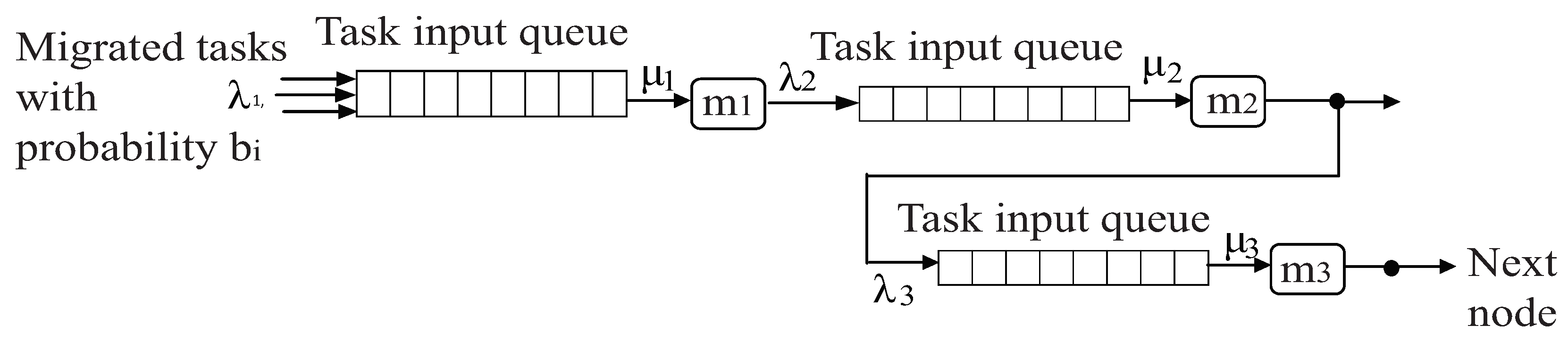
The Maximum Acceptable Input Arrival Rate for Migrated Tasks We can assume that the nodes of a cluster are loaded with migrated tasks based on distance to the source that previously accommodated these tasks and based on an acceptable input rate. Clearly, we need to distribute the migrated tasks from their host node to nodes of close proximity while maintaining the data input rate of these nodes (do not overload them). To examine the input rate, a simple model is proposed: First, the nodes current state is expressed as a vector $\mathbf{K}=(K_1,K_2,\cdots ,K_m)$, where $K_m$ is the buffer space available to accommodate newly migrated tasks in node m [30]. The buffer size is measured in terms of the number of tasks it occupies. The conditional probability of moving from state $\mathbf{K}$ to ${\mathbf{K}}^{\prime }$ is denoted by $p(\mathbf{K},\tau |\mathbf{K},\tau +\delta )$, where $\tau$ denotes the time and $\delta$ is a period long enough to accommodate only one change of state. The overall probability of reaching a state ${\mathbf{K}}^{\prime }$ is

$$p(K_1^{{}^{\prime }},K_2^{{}^{\prime }},\dots ,K_m^{{}^{\prime }})=p_1\left(K_1^{{}^{\prime }}\right)·p_2\left(K_2^{{}^{\prime }}\right),\dots p_m\left(K_m^{{}^{\prime }}\right)$$

(9)

where $p_m{K}_m^{{}^{\prime }}$ is the probability of a node’s buffer to have $K_m^{{}^{\prime }}$ space. The $p_m$ values indicate the utilization of a node m and it is computed by

$$p_j=\frac{{\lambda }_m}{{\mu }_m}\le 1$$

(10)

where ${\mu }_m$ is the mean forwarding time (or service time) for the migrated tasks relayed to node m and the $\lambda$ values are the mean input rates of tasks to the nodes. Each ${\lambda }_m$ is a sum of the form

$${\lambda }_m=b_{m-1}{\lambda }_{m-1},$$

(11)

where $b_{m-1}$ is the probability of task migrations to node $m-1$. For example, see Figure 1 and consider the parameter values of

Table 3. Parameters for the task migration example of Figure 1.

Parameter	Symbol	Value
Mean arrival rate an node $m_1$	${\lambda }_1$	30 tasks/s
Mean service time at node $m_1$	$1/{\mu }_1$	20 ms
Mean service time at node $m_2$	$1/{\mu }_2$	25 ms
Mean service time at node $m_3$	$1/{\mu }_1$	40 ms
Probability of task migrations through $m_1$	$b_1$	0.25
Probability of task migrations through $m_2$	$b_2$	0.3
Probability of task migrations through $m_3$	$b_3$	0.4

. Then, Equation (11) would produce ${\lambda }_2=15$ tasks/s and ${\lambda }_3=20$ tasks/s. Then, from Equation (10), $p_1=\frac{30\times 20}{1000}=0.6$, $p_2=\frac{15\times 20}{1000}=0.3$, and $p_3=\frac{20\times 40}{1000}=0.8$. Then, the maximum acceptable input rate per node is the one that saturates it, for example $m_1$ is saturated for ${\lambda }_m>50$ tasks/s because $(50\times 20)/1000=1$.

Fair Distribution of the Migrated Tasks By “fair distribution”, two things are meant: (1) fairness in terms of distance between nodes, that is, the nodes located closer to the source of migrated tasks should take more load to keep the communication cost to the minimum, and (2) fairness in terms of the load itself, that is, the load of the migrated tasks should be distributed as evenly as possible taking into consideration the maximum acceptable input rate and the nodes distance. To distribute the tasks fairly, we use the following simple three-stepped procedure:

Step 1:Find the maximum number of tasks$U_{jmax}$ that can be re-allocated to each node: This number is dependent on the total utilization of each node at the current time, that is, on the acceptable input rate discussed previously (see Equation (10)).

$$U_{jmax}=T\times p_j$$

(12)

where T is the total number of migrated tasks.

Step 2:Divide the number of migrated tasks by the sum of the maximum number of tasks that can be re-allocated to all the nodes based on their utilization.

$$f=\frac{T}{{\displaystyle \sum _{j=1}^m{U}_{jmax}}}$$

(13)

This will produce an analogy of the number of migrated tasks compare to the number of tasks that the system can re-accommodate based on its node utilization.

Step 3:Compute the loading factor per node:

$$F_j=U_{jmax}\times f$$

(14)

The loading factor will decide about the total number of migrated tasks each node can accommodate.

For the example of Figure 1, if $T=50$ and the utilization values yielded are $p_1=0.6,p_2=0.3$, and $p_3=0.8$, then $U_{1max}=50\times 0.6=30$, $U_{2max}=50\times 0.3=15$, and $U_{3max}=50\times 0.8=40$. The sum of the $U_{jmax}$ values is $30+15+40=85$ and the f value is $50/85=0.58$. Then, the F values are $F_1=30\times 0.58=17.4$, $F_2=15\times 0.58=8.7$, and $F_3=40\times 0.58=23.2$. Thus, the 50 migrated tasks would be re-allocated as follows: 18 to node $m_1$, 9 to node $m_2$, and 23 to node $m_3$.

Two things are worth noticing:

1.

The model presented for fair redistribution of the migrated tasks monitors the load per node. Under the assumption that the tuples distributed are of equal size (this is quite natural and many times desirable), then because of the stepwise strategy of our scheduling, the node utilization values would be very close. This would produce even and fair task redistribution. For different sized transmitted tuples, again there is a guarantee that big parts of the cluster would remain balanced in terms of load processing.

2.

The method can be expanded to a larger number of clusters or networks by using relay nodes that connect different clusters. We will explain this when we present our experimental results.

Finally, note that, as a result of the queuing approach of our fair task re-allocation policy, there is some type of exponential effect on the system’s throughput (see [30]).

5. Pipelined Scheduling

This section shows how to pipeline the main procedures involved in a data stream processing problem. The overall work required by data stream processing applications is divided into three stages: The transferring stage is the stage at which data streams are forwarded according to the communicating steps defined by the $FSM$ of Section 3 and $B_1$ is used to denote the maximum-cost communication step. The processing stage is the stage at which the streams are processed by the nodes. In this context, we will assume with no loss of generality that all the data streams are considered equal so processing is implemented in constant time $B_2$. Finally, the packing stage is the stage at which the resulting processed streams are put into buffers, in order to be forwarded to the next nodes for further processing. This is the fastest stage. The packing time is $B_3$, and is equal for all the streams being processed. It should be noted that the migrated task go through these stages as well.

In the analysis that follows, some communication steps are more expensive compared to the actual stream processing (apparently the ones that involve nodes placed far apart), while others are less expensive. Thus, $B_1>B_2>B_3$. Other cases that may arise (for example all communication steps are “cheaper” or “more expensive” than the processing costs) can be examined similarly.

In Figure 2, the gray areas indicate pipeline stage stalls, that is, a stage has no work to do and waits until it becomes busy again. The “fade to black” areas indicate the work being implemented for migrations. Let two communication steps, $S_0,S_1$, have the maximum cost $B_1$ and let there be two task migrations. Since $B_1>B_2$, the streams with maximum cost are transferred in $2u$ time, while their processing will have finished at time $2B_1+B_2$. The next two steps $S_2,S_3$, require $B_4$ time, where $B_4<B_1$, but $B_4>B_2$. This means that their transfer would be completed at times, $2B_1+B_4$ and $2B_1+2B_4$, respectively, while their processing will have finished at times $2B_1+B_4+B_2$ and $2B_1+2B_4+B_2$, respectively. The communication steps $S_4,S_5$ require $B_5$ and $B_6$ time, where $B_1>B_5>B_6$. The transfer stage for $S_4$ and the processing stage for $S_3$ start at time $2B_1+2B_4$, but the streams of $S_4$ would be transferred by $2B_1+2B_4+B_5$, while the processing of $S_3$ which started simultaneously ends later, at time $2B_1+2B_4+B_2$. Finally, the streams of $S_5$ will be transferred by $2B_1+2B_4+B_5+B_6$ and during that time, the processing $S_4$ streams takes place. It takes $2B_1+2B_4+B_5+B_6+B_2$ to transfer, process, and pack all the streams involved in steps $S_0-S_5$. Now, assume that there are two task migrations. In our scheme, to achieve synchronization, we start them immediately after transferring the streams for $S_5$. Thus, we always kill the tasks found in the former hosts of the migrated tasks, after the completion of the scheduled communication steps and after the completion of the task migration. The nodes that will accommodate the migrated tasks are determined as shown in Section 4. The migrated tasks are also transferred using the communication scheme described in Section 3 and impose at most (assuming these migrations have the maximum cost $B_1$ plus an extra overhead $B_7$ for the checkpoints) an extra latency of $\rho B_1+\rho B_7$. An approximation to the total cost $TC$ is:

$$TC=(\rho +2)B_1+(k-2)B_4+B_5+B_6+B_2+B_3+\rho B_7$$

(15)

where k is the number of communication steps and $\rho$ is the number of times migrations are needed. Recall that, by employing this pipelined organization, some processing/packing costs are actually “absorbed” resulting in reduced overall delays. This will be shown in the next section.

6. Simulation Results and Discussion

The proposed task migration policy is evaluated using a simulation environment, which provides a wide range of choices to develop, debug, and evaluate their experimental system. In our experimental setup, the Storm cluster consists of nodes that run Ubuntu 16.04.3 LTS with an Intel Core i7-8559U Processor system, and clock speed at 2.7 GHz, 1 Gb RAM per node. Further, there is all-to-all communication between the nodes, which are interconnected at a speed of 100 Mbps. Experiments were conducted on a linear application topology, with four bolts and one spout, where the number of tasks per component varied from 4–16. As the cluster size expanded, our last experiments were implemented on a cluster of 100 nodes with a total number of 600 tasks running in total. The overall cluster was always divided into sub-clusters of $Q=5$ nodes, although similar results can be obtained with any other division of the cluster. The tuples are text datasets and the application used for the experiments is the typical word count example. The tuples are associated to simple text datasets. The application we used for our simulations is the typical word count example. For example, one task processes a tuple and seeks for all the words starting from a selected letter. Then, it passes the processed tuples to a next task, which in turn, seeks for a word that starts with a combination of the selected letter and a few more letters. Proceeding in this way, the application performs word counting on large datasets. The application is run in parallel to a number of sub-clusters

To show how the scheme worked on larger clusters, see the example of Figure 3:

There are two cases:

• A task migration involves (this decision is based on the model of Section 4 based on link monitoring) only the nodes of a sub-cluster (for example, task migrations from a node to the other nodes of sub-cluster 1). Then, a redistribution with parameters $N=Q=5,t,s,s>t$ was executed. For example, if our fair distribution model decided to redistribute 8 migrated tasks to 4 nodes with initial distribution of 4 tasks per node, then the redistribution parameters would be $N=Q=5$ (recall that we kept each sub-cluster equal to 5 nodes), $t=4,s=4+\frac{8}{4}=6$.
• A task migration involves moving tasks from one sub-cluster to another. Again, the same type of redistribution was used. For example, assume that we need to migrate 8 tasks from a node of sub-cluster 1 to 4 nodes of sub-cluster 2 of Figure 3. Again, a redistribution with parameters $N=Q=5,t,s,s>t$ was executed but this time with larger transfer times. Then, the communications can continue using the communication scheme of Section 3.

The parameters we measured in our experiments are the load balancing and the overall latency. We used two state-of-the-art new strategies for our comparisons: (1) The approach of Shukla et al. [22], an approach that deals with task migrations and reduces the extra latencies that incur from incremental flows of checkpoint messages and their full processing and (2) the MT-Scheduler presented by Sinayyid and Zhu [31]. This work is a fast technique that uses a dynamic programming scheme to efficiently map a DAG onto heterogeneous systems. This scheme achieves system performance optimization (throughput rate maximization) by estimating and minimizing the time incurred at the computing and transfer bottlenecks and it is a good candidate for latency comparisons.

Load Balancing

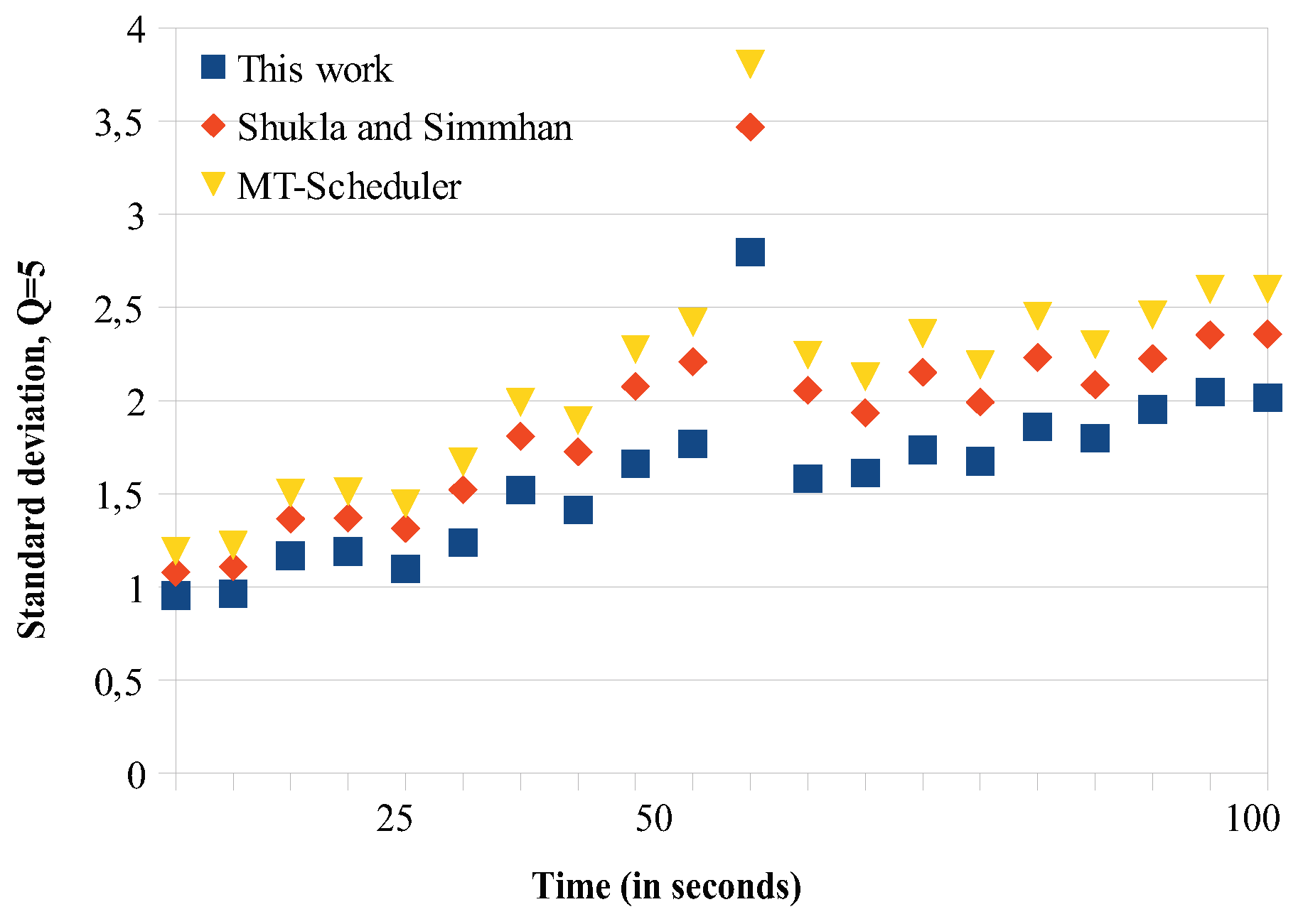
We conducted two sets of experiments regarding load balancing. In the first set, we try to find how the migrations affect the load balancing, so we computed the latency during the migration periods. The overall migration process required from 10 to 100 s, depending on the number of tasks migrated and the corresponding data (tuples) that they processed. We repeated the migration experiment for 20 times and for different cluster sizes and we regularly computed (every 5 s) the average standard deviation of the load being delivered to each node (see Figure 4, Figure 5, Figure 6 and Figure 7). An increase of the standard deviation value indicated less load balancing among the system’s nodes.

The approach of Shukla and Simmhan is based on using the link information through dataflow checkpoints. A timeout period is employed, where no data but only in-flight messages are transmitted. The timeout regulation helps Shukla’s and Simmhan’s to have somehow better balancing results compared to the MT scheduler, as Figure 4, Figure 5, Figure 6 and Figure 7 show. In the MT-Scheduler, the only regulation policy used is that the users are allowed to configure and regulate the data locality, in order to maintain execution of the tasks as close to the data. This cannot guarantee load balance. As Figure 4, Figure 5, Figure 6 and Figure 7 show, this strategy suffers from higher imbalances. Our work was found to have smaller standard deviation values compared to the other schemes, thus better balancing. For the communications implemented within each sub-cluster, there is a one-to-one communication among the system nodes. Some imbalances incur (notice that some points have higher values as seen in Figure 4, Figure 5, Figure 6 and Figure 7) in cases when some nodes are somehow more overloaded and the migrated tasks are not evenly redistributed to maintain fairness. However, one can notice that, because our communication strategy generally keeps load balancing among the nodes, there are only a few of these points.

In the second set of experiments, we compute the average load balancing for a period of one hour (3600 s). Specifically, Figure 8a shows the average load balancing for clusters of at most 50 nodes, while Figure 8b presents the load balancing results for a cluster of 50–100 nodes. Apparently, as more and more data streams are generated and more migrations are involved, all the proposed schemes will suffer larger imbalances. Still, our scheme manages to have smaller increases in the standard deviation value. Notice in Figure 8a,b that the curve corresponding to our scheme appears to be growing slow and rather smoothly, as a result of the stepwise communication strategy being employed.

7. Average Latency

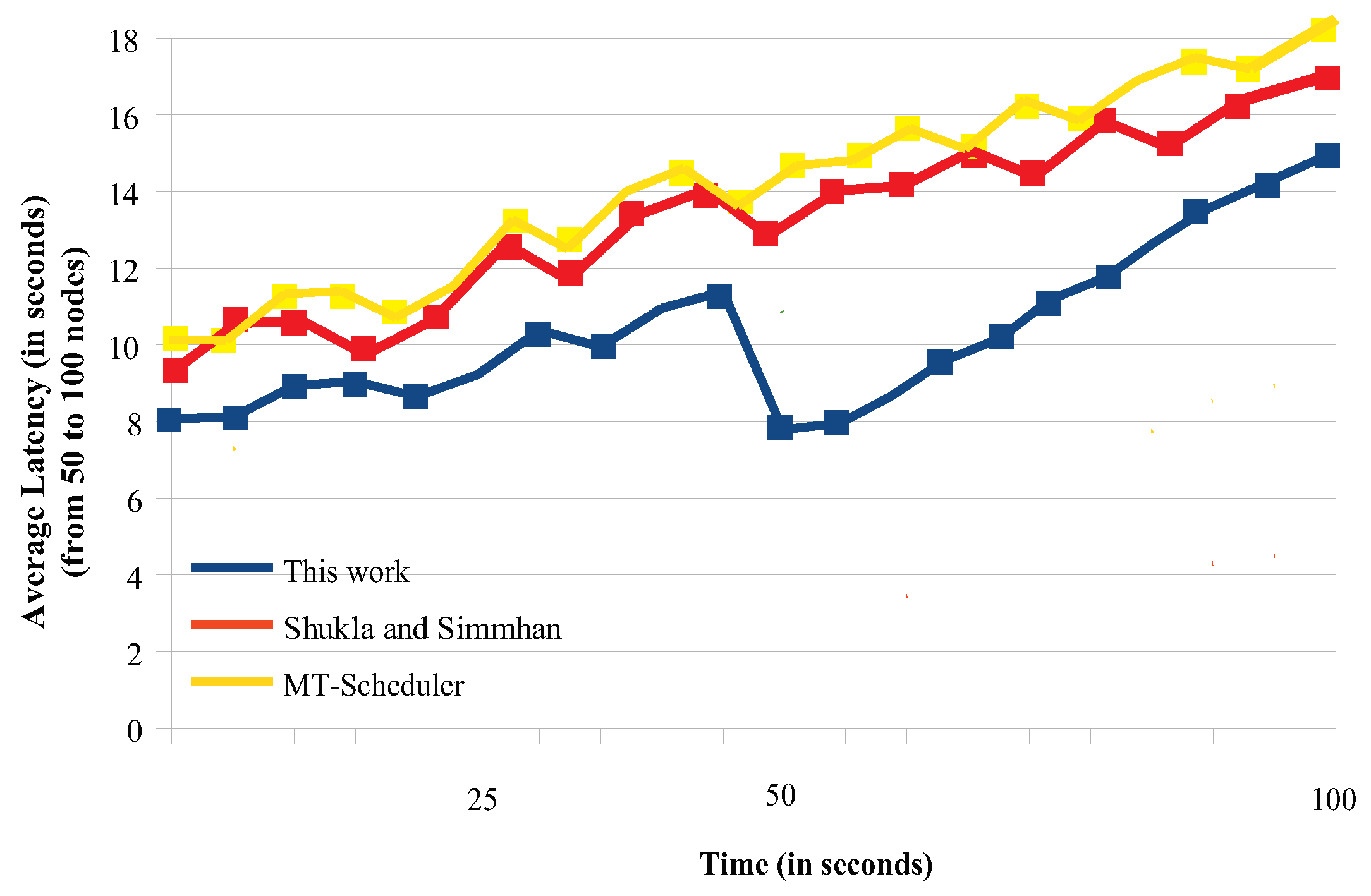
To study the average latency, we conducted two sets of experiments. In the first set, we try to find how the migrations affect the total latency, so we computed the latency during the migration periods. Again, the overall migration process required from 10 to 100 s, depending on the number of tasks migrated and the corresponding data (tuples) that they processed. We repeated the migration experiment 20 times for clusters of 5–50 and 50–100 nodes (we gradually expanded the network size by adding subclusters) and we regularly computed (every 5 s) the average latency (see Figure 9 and Figure 10).

The small ups and downs that one can see indicate that, every time we expanded the network (added another sub-cluster) and redistributed the tasks, we got a latency drop for a short period of time, but as more data kept arriving, this small gain was eliminated and the latency increased. As an example, notice, in Figure 10, the large drop of the latency found in our scheme, when we expanded the network size from 85 to 100 nodes, at time ≈ 45 s. This latency reduction lasted for a few seconds. As more and more data streams kept arriving, the latency gradually increased.

For our strategy, one can notice that the latency increases in a rather smooth way, especially for smaller networks (see Figure 9). As the network size and the number of tasks further increase, so does the latency for all the schemes (see Figure 10). Particularly, Shukla’s and Simmhan’s scheme had almost identical behavior for smaller and larger networks (see the shape of the 2 curves in Figure 9 and Figure 10), but the latency experienced for larger networks was quite larger. This can be explained by the regular timeouts employed in this scheme. Although the MT scheduler optimizes the system performance, it incurs regular and large imbalances when task migrations occur and thus, under such conditions, it experiences the largest latencies.

In the second set of experiments, we study the overall latency for a period of one hour. The results are shown in Figure 11a,b, for networks of 5–50 and 50–100 nodes. Again, our work outperforms its competitors for two main reasons: (1) the buffering required by our scheme is minimized because the communications are performed in such a manner that each node gets data from only one node at a time. On the long term, when there are large amounts of unprocessed data buffered, the latency increases, and (2) the overlapping of certain communication and processing procedures.

8. Conclusions-Future Work

This work presented a dynamic scheduling scheme to handle task migrations in large-scale networks. The approach is organized in a set of communication steps, where there is an one-to-one communication between the system’s nodes. Then, it uses a new probabilistic model to estimate the acceptable migrated task input rates and finally, the basic stages involved in stream processing are pipelined and thus, latencies are reduced. The task migrations are efficiently handle by this type of scheduling. Another advantage of our work, as the simulations have shown, is that it can be expanded to larger networks divided into relatively small clusters. The simulation results have verified that the proposed scheme offers better load balancing and reduces the overall latency compared to state-of-the-art schemes.

In the future, this work will be extended to test the scheduler’s performance on even larger clusters and on different application topologies (like diamond, or random topologies). Moreover, other fair allocation policies are examined. In addition, one of the key considerations in big data management is fault-tolerance which may overturn the whole process’s effectiveness. Our future work will also consider this point in our testing experiments. Finally, we investigate the possibility of integrating the fair scheduling approach to other well-established schedulers.