Hair Removal Combining Saliency, Shape and Color

Featured Application

Hair removal is a preliminary and often necessary step in the automatic processing of dermoscopic images since hair can negatively affect or compromise the distinction of a lesion region from the normal surrounding healthy skin. A featured application is skin lesion segmentation.

Abstract

In a computer-aided system for skin cancer diagnosis, hair removal is one of the main challenges to face before applying a process of automatic skin lesion segmentation and classification. In this paper, we propose a straightforward method to detect and remove hair from dermoscopic images. Preliminarily, the regions to consider as candidate hair regions and the border/corner components located on the image frame are automatically detected. Then, the hair regions are determined using information regarding the saliency, shape and image colors. Finally, the detected hair regions are restored by a simple inpainting method. The method is evaluated on a publicly available dataset, comprising 340 images in total, extracted from two commonly used public databases, and on an available specific dataset including 13 images already used by other authors for evaluation and comparison purposes. We propose also a method for qualitative and quantitative evaluation of a hair removal method. The results of the evaluation are promising as the detection of the hair regions is accurate, and the performance results are satisfactory in comparison to other existing hair removal methods.

1. Introduction

In almost every specialist area of medicine, including dermatology, image analysis is transforming the diagnostic methods. In particular, computer-aided diagnosis systems for dermoscopic images have proven to be useful tools to improve significantly the common dermoscopic diagnostic practice, which is usually characterized by limited accuracy and is mainly based on visual inspection. Indeed, to differentiate melanoma from other pigmented skin lesions, these systems display morphological features not easily perceptible by the naked eye and support the assessment process of the human expert [1,2]. Typically, a computer-aided system is structured in four main consecutive steps: preprocessing, segmentation, feature extraction, and classification, each playing a key role in enabling correct diagnosis [3]. During the preprocessing, the dermoscopic image is subjected to noise removal, image enhancement, color quantization, and artifacts removal processes [4,5]. Noise removal and image enhancement techniques are employed to minimize the effects due to different illumination conditions and poor resolution of the acquisition process [6]. Color quantization [7,8,9,10] is a technique of reducing the total number of unique colors in the image often used as a preprocessing step for many applications that are carried out more efficiently on a numerically smaller color set. For example, color quantization is employed effectively as a preliminary computation phase for skin lesion segmentation [11,12,13,14,15]. The removal methods of artifacts, such as bubbles, hair, shadows and reflections, aims to eliminate their negative effect and disturbance on the diagnostic operations of the area of interest (i.e., the skin lesion) [16]. Particularly, if the area of the skin lesion is partially occluded by the hair, although such occlusions may not be critical for human investigation, this presence poses major challenges for automatic image analysis method such as segmentation and classification. Indeed, the hair removal (HR) methods and skin lesion segmentation (SLS) methods are highly correlated. Usually, SLS methods can determine the skin lesion region without the need to apply preliminary hair removal since these methods can include explicitly or implicitly hair removal operations. However, it is appropriate to consider that (a) in any case, a partial hair removal facilitates and increases the efficiency of the segmentation step; (b) the hair presence can lead to errors in lesion detection in some situations, especially when there is a massive presence of hair (see Figure 1); (c) for diagnostic and therapeutic purposes, HR is helpful at least to visualize the free-hair lesion to the expert.

To address the hair issue, several hair removal methods have been proposed. HR methods usually consist of two steps: (a) the detection of occluding hair and generation of the hair binary mask; (b) the removal of the detected hair. Typically, hair detection is accomplished through object detection methods enucleating thin items, while hair removal is obtained through standard inpainting methods. As reported in [17], at least six main hair removal methods are widely used in the literature [18,19,20,21,22,23].

The method proposed in [18] by Lee et al., also known as Dullrazor, consists of four steps. The hair regions are initially detected through the morphological closing operator on each RGB color channel separately and with three structuring elements having different directions (step 1). To generate the binary mask, a thresholding process is applied to the absolute difference between the original color channel and the image generated by the closing (step 2). The mask pixels undergo a bilinear interpolation between two nearby not-mask pixels (step 3). Finally, to the resulting image, an adaptive median filter is applied (step 4).

The method [19] by Xie et al. also consists of four steps. The hair area is improved using a morphological closing top-hat operator (step 1). The binary image is obtained through a statistical thresholding process (step 2). To extract the hairs, the elongate feature property of connected regions is employed (step 3). To restore the information occluded by the hair, they apply the image inpainting method based on partial differential equation (PDE), which realizes the diffusion of information through the difference between pixels (step 4).

In the method proposed in [20] by Abbas et al., there are three computational steps. In the CIELab uniform color space, the hairs are detected by a derivative of Gaussian (DoG) (step 1). Morphological techniques to link broken hair segments, eliminate small and circular objects, and fill the gaps between lines are applied (step 2). The adopted inpainting method is based on coherence transport (step 3).

The method in [21] by Huang et al. comprises three steps. To the grayscale version of the image, a multiscale curvilinear matched filter is applied (step 1). To detect the hair regions, hysteresis thresholding is employed (step 2). Then, region growing and the linear discriminant analysis (LDA) technique, based on the pixel color information in the CIELab color space, are applied to recover the missing information left by the removed hair (step 3).

The method [22] by Toossi et al. includes four steps. The image is converted to a grayscale image via a principal component analysis (PCA), and the noise is filtered with a Wiener filter (step 1). Hair is detected by using an adaptive canny edge detector (step 2). A refining process with morphological operators to eliminate unwanted objects and obtain a smooth hair mask is then applied (step 3). The inpainting process is carried out by a multi-resolution transport inpainting method based on wavelets (step 4).

As with [20,21], in [23] by Bibiloni et al., hair removal is made up of three steps. The contrast of the luminance of the image is improved with the Contrast Limited Adaptive Histogram Equalization (CLAHE) algorithm (step 1). The hair is detected using soft color morphology operators in the CIELab color space (step 2). The inpainting phase is based on the arithmetic mean of the modified opening and closing morphological transformations to recover the missing pixels (step 3). The common element of these HR methods and most of the other existing methods, e.g., [24,25], is the employment of morphological operations and, to a minor extent, of information derived from color. On the other hand, although deep learning has been used successfully to solve many difficult computer vision problems, inexplicably, to the best of our knowledge, only two very recent HR methods relying on neural network architecture exist [26,27].

Despite the sufficiently wide variety of the existing papers, the problem of hair removal results to be not solved satisfactorily yet. The main critical points are the failure to identify hair accurately and the undesirable effects such as unremoved thin hair and color alteration.

We address the HR problem using information regarding the saliency, shape, and color of the image objects. These are three elements that have proved to be extremely useful because each of them allows capturing a fundamental aspect of the problem at hand. Indeed, besides the shape aspects, detectable by mathematical morphology properties, it is also appropriate to perform the hair detection based on information related to the significant image elements and detectable by their saliency and color properties. In the following, we refer to the proposed method as saliency shape color for hair removal, shortly indicated as HR-SSC or simply SSC.

As described in Section 2, HR-SSC consists of five steps. The core of the method is step 4, named hair object detection, in which the hair regions are determined. The innovative elements of this step, whose success also depends on the correctness of the results obtained in the three previous steps, are related mainly to how the initial candidate hair components are considered (see Section 2 for more details). In the last step, hair removal is performed using a standard inpainting method.

The method is evaluated and compared extensively with other existing methods since a detailed quantitative and qualitative analysis on two publicly available databases PH² [28] and ISIC2016 [29], usually used in dermoscopic image processing, is performed.

The experimental results confirm (a) the effectiveness and the utility of the employment of saliency, shape, and color information for HR; (b) that HR-SSC achieves good quantitative results with an adequate balance and has a competitive and satisfactory performance concerning other existing HR methods; (c) that HR-SSC implementation is simple and rather fast since it does not require a large amount of computational power based on a high number of parameters and of labeled training images.

Additional contributions of this work are (a) the availability of appropriate datasets to be used for testing and comparing each new method; (b) the proposal of a method for qualitative and quantitative evaluation of an HR method.

The paper is organized as follows: in Section 2, we describe the method HR-SSC, detailing its main steps; in Section 3, we provide a quantitative and qualitative evaluation of experimental results, also highlighting the pros and cons; finally, discussion and conclusions are drawn in Section 4.

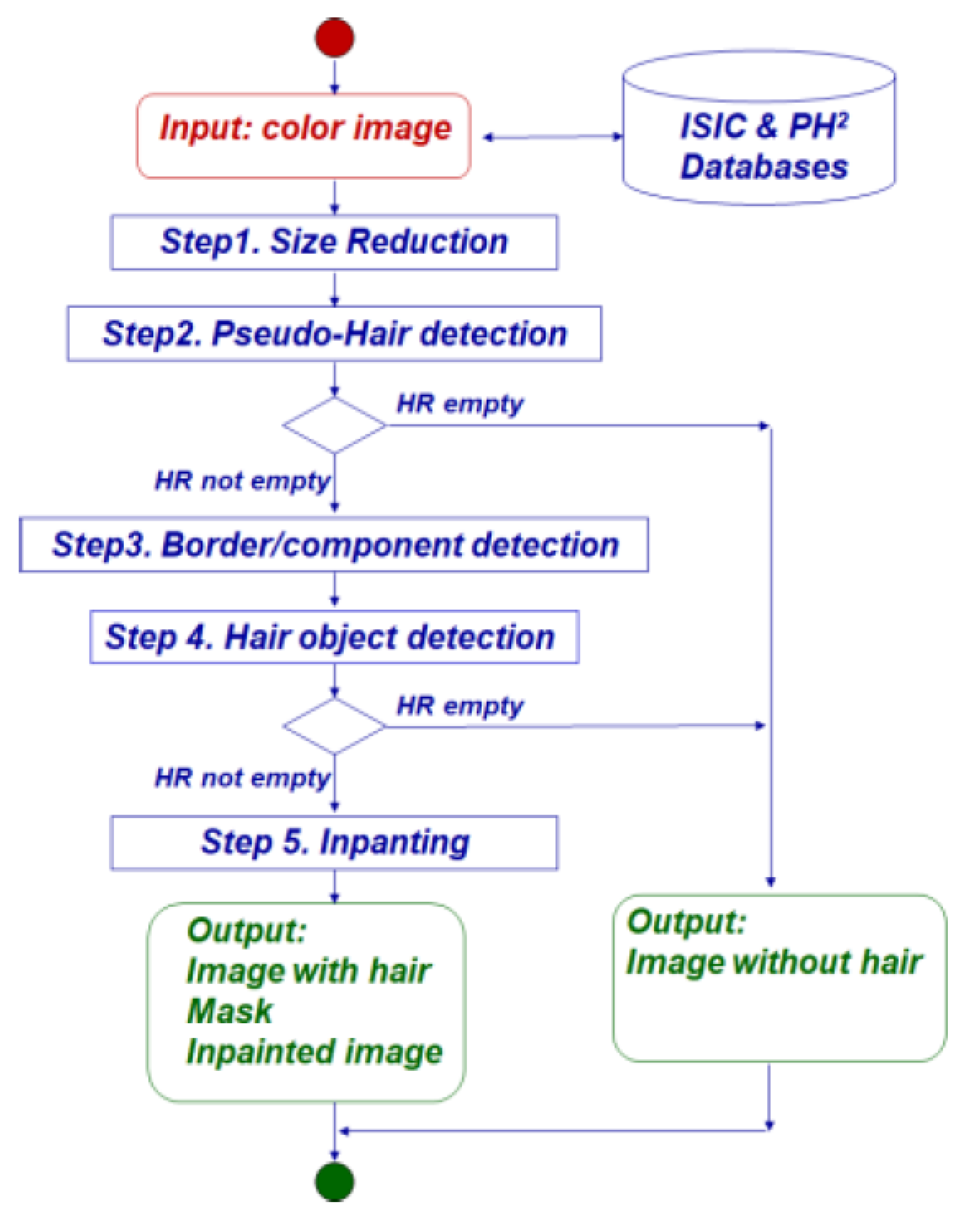
2. The Proposed Method

The proposed method, as mentioned above, is based on three elements: the notion of visual saliency, shape, and color. Indeed, since the saliency of an item is the element for it stands out from its neighbors [30], its use allows to enucleate the most relevant subsets and to focus on the hair regions especially. Moreover, since hair regions have a well-defined structure, the shape-oriented operations of the mathematical morphology, that “simplify image data, preserving their essential shape characteristics and eliminating irrelevancies” [31], lend themselves well to detect the hair object. On the other hand, the properties of the color model can result essential to distinguish between no-hair and hair regions when information related to saliency and shape is not enough to manage ambiguous cases [11].

The method consists of five main steps as described in the diagram shown in Figure 2. The step “Hair object detection” is the main step and is preceded by three preliminary steps, called “size reduction”, “Pseudo-Hair detection” and “Border and corner component detection” aimed respectively at reducing the image size, determining the initial candidate regions to consider as hair regions, called pseudo-hair, and determining the components located on the frame of the image. The “Hair object detection” step is followed by the hair removal step and the resizing called “Inpainting and rescaling”. Specifically, the method can be briefly described as follows.

Step 1. 

Size reduction—The first step is devoted to limit the computation burden of the successive steps by reducing the size of the input image with a scale factor s equal to the ratio of a fixed value, say Maxdim, and the number of columns. To perform this, we resort to the classical and most common bicubic downsampling, implemented by the Matlab command imresize with bicubic option and scale factor s. The size reduction step is an optional but highly recommended operation since it significantly limits the computation time.

Step 2. 

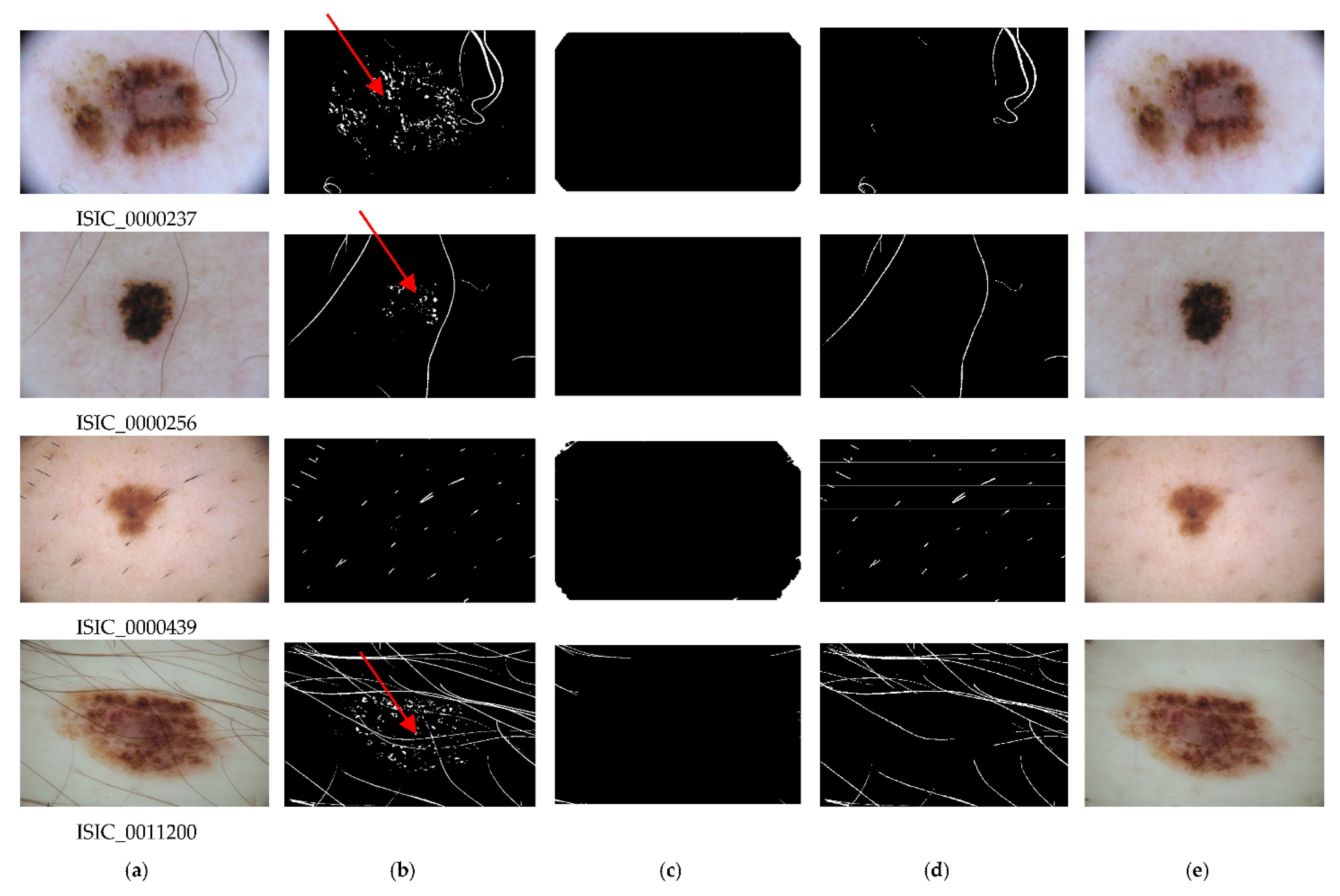
Pseudo-Hair detection—This step is based on top-hat transformation, i.e., a morphological operator capable of extracting small elements and details from a grayscale image, commonly used for feature extraction, background equalization, and other enhancement operations. There are two types of transformation: the white top-hat transformation, defined as the difference between the original image and its aperture by a structuring element, and the black top-hat transformation (or bottom-hat transformation), defined dually as the difference between the closure by a structuring element and the original image [32,33]. Following [19,34], to obtain the binarized version HR initially containing the pseudo-hair components, we apply a bottom-hat filter in the red band R of the RGB image and then the Otsu threshold method [35] by the Matlab command imbinarize. Then, if HR is not empty, the actual hair regions are determined during the successive steps 3–5.

Indeed, the components currently detected in HR (i.e., the so-called pseudo-hair components) can correspond to hair regions but can also correspond to portions of other types of artifacts survived this preliminary treatment, such as marker ink signs, dark spots belonging to the lesion, marker colored disks [34], and regions wrongly identified. These regions not corresponding to hair regions are called no-hair regions in the following, and if they exist, they are detected and eliminated in the successive steps. In Figure 3b some examples of pseudo-hair are shown, where the no-hair regions are approximatively indicated by a red arrow.

Step 3. 

Border and corner component detection—The border components are detected based on their saliency and proximity to the image frame, by applying the following process, named called border detection, already used in [14,15]. The saliency map (SM) with well-defined boundaries of salient objects is computed by the method proposed in [36]. Successively, SM is enhanced by increasing the contrast in the following way: the values of the input intensity image are mapped to new values obtained by saturating the bottom 1% and the top 1% of all pixel values, by the Matlab command imadjust. Then, the saliency map SM is binarized by assigning to the foreground all pixels with a saliency value greater than the average saliency value. The connected components of SM including pixels of the image frame are considered as border components and stored in the bidimensional array, named BC.

Moreover, the image corner components, usually much darker than the image center, are detected following the same procedure proposed in [34]. Specifically, the representation of the input image in the HSV color space is examined; the channel V undergoes a thresholding process by a predefined threshold value δ. Then, the components of the thresholded V covering most of the frame or the corner area of the image are considered as image corner components and are stored in the bidimensional array, named CC (see Figure 3c).

Step 4. 

Hair object detection—Preliminarily, the no-hair regions are detected and stored in the bidimensional array, named NR, as follows. NR is initially computed as the product S.*V and binarized by the Otsu method. Then, the salient pixels not belonging to HR and BC are included in NR, the pseudo-hair regions currently detected in HR are removed from NR, and small holes in NR are filled. Successively, if NR has a significant extension (area), the detected no-hair regions are removed from HR. If the current HR is not empty, border components are suitably considered and possibly removed from HR taking also into account the gray version of the input image Ig and a fixed gray value, say Δ, indicating a minimum reference gray value for the hair component. Finally, corner components and eventual remaining components corresponding to colored disks are eliminated from HR.

At the end of this step, the regions in HR are located in correspondence with the detected hair objects and form a binary hair-mask on which to perform the next reconstruction step. See the Matlab pseudocode given below for more details. In Figure 3d, examples of detected hair are given.

Step 4. Hair object detection

% No-hair regions detection NR = S. *V; % Initial no-hair regions construction and storing in NR NR = imbinarize(NR, graythresh (NR)) % Otsu binarization

NR(SM > 0 & HR == 0 & BC == 0) = 1; % insertion in NR of salient pixel not belonging to HR and BC

NR (HR > 0) = 0; % pseudo-hair elimination from NR

NR = imfill(NR,’holes’); % holes filling % end of no-hair regions detection

if (area(NR) is significant)

HR(NR > 0) = 0; % no-hair regions removal from HR

HR = imfill(HR,’holes’); % holes filling

if (HR is not empty)

if (BC is not empty) % border and corner components management

NB = BC; % copy of BC

NB(NR > 0 & Ig > Δ) =0 ; % generation of NB without no-hair regions and too dark regions

HR(NB >= 0 & SM > 0) % elimination of salient pixels of NB from HR

CR = (BC > 0 & NB > 0) % common regions to BC and NB

HR(CR > 0) = 0 % elimination from HR of common regions of BC and NB

CR(CR > 0 & CC > 0) = 0; % corner regions elimination from CR

BN = border_detection (CR); % border components detection in CR (as done in step 3)

if (BN is not empty)

HR(BN > 0 & Ig > Δ) = 0; % elimination of clear border regions of CR from HR

end

end

HR(NR > 0 & HR > 0 | (BC > 0 & Ig > Δ)) = 0; % colored disk and clear border component removal

end

end

Step 5. 

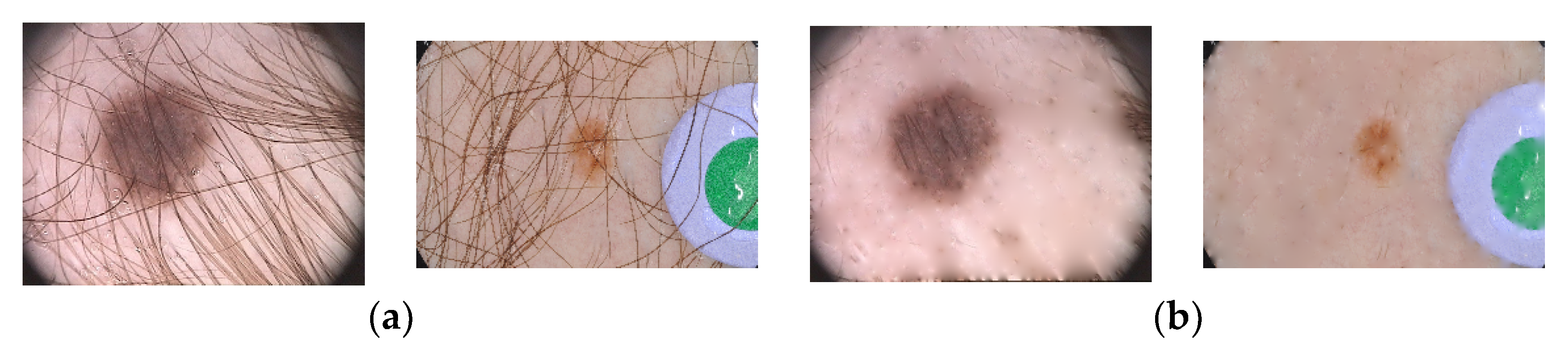
Inpainting and rescaling—If HR is empty, the image is considered hairless; otherwise, the reconstruction process is applied. After a preliminary enlargement of HR by n steps of dilation, the inpainting is carried out by calling the Matlab function regionfill on each image channel separately, by using HR as hair-mask and then joining the resulting channels. If the size reduction step has been performed, a scaling is newly applied using the Matlab function imresize with the bicubic option. In Figure 3e, examples of the resulting image are given.

Different parameter settings to achieve a trade-off between quality and performance have been explored. The better parameter values resulting from this analysis are Maxdim = 500, δ = 0.4, Δ = 100, n = 3. The experimental results shown in this paper are obtained by this setting. The method is implemented in Matlab using Intel^® core ™ i7—6600U CPU 2.60 GHz with 8 GB installed RAM and a 64-bit Operating System Windows 10.

3. Experimental Results

This section describes the image datasets and the evaluation of the experimental results in qualitative and quantitative terms. In fact, the evaluation of the performance of the proposed method and the comparison with other methods are very hard tasks due to the lack of publicly available source code of the existing methods, the limited literature, and the different evaluation methodology often employing not well-specified datasets and different quality measures. To overcome these critical issues, (a) we select some adequate datasets (see Section 3.1); (b) we perform qualitative evaluations/comparisons from different points of view (see Section 3.2); (c) following [17,37], we perform quantitative evaluations and comparisons by generating synthetic hair on skin lesion images originally hair-free in a controlled way (see Section 3.3). Note that the controlled hair introduction modality offers the advantage that the added hair regions are known and constituted a reference image, i.e., a ground truth. Accordingly, since the quantitative evaluation of the performance of an HR method requires a reference image, this modality is the unique way to evaluate the results by comparing the added hair regions in the reference image (ground truth) with the detected hair regions in the binary mask.

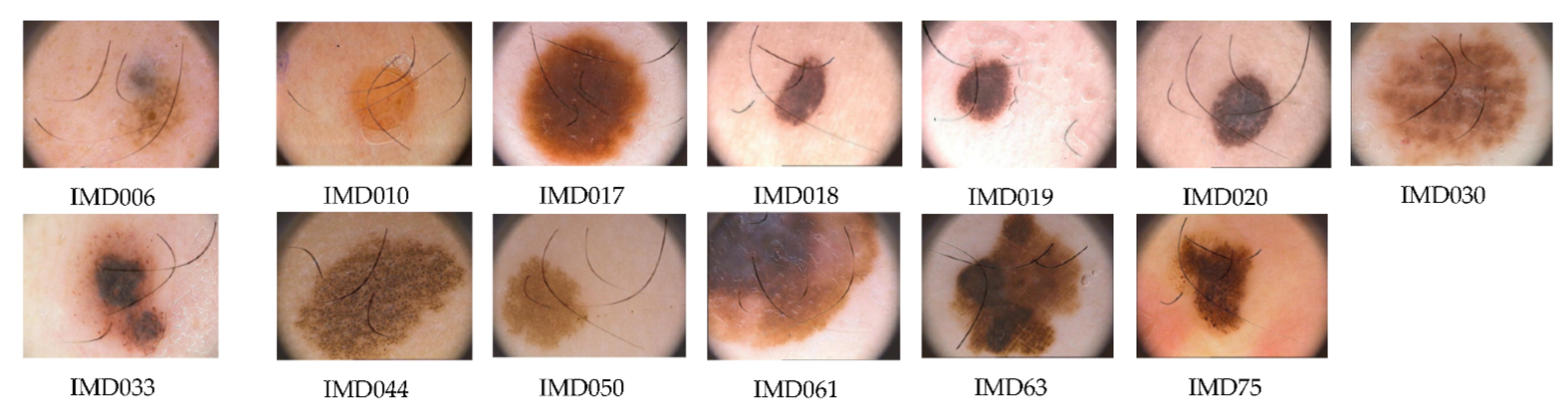
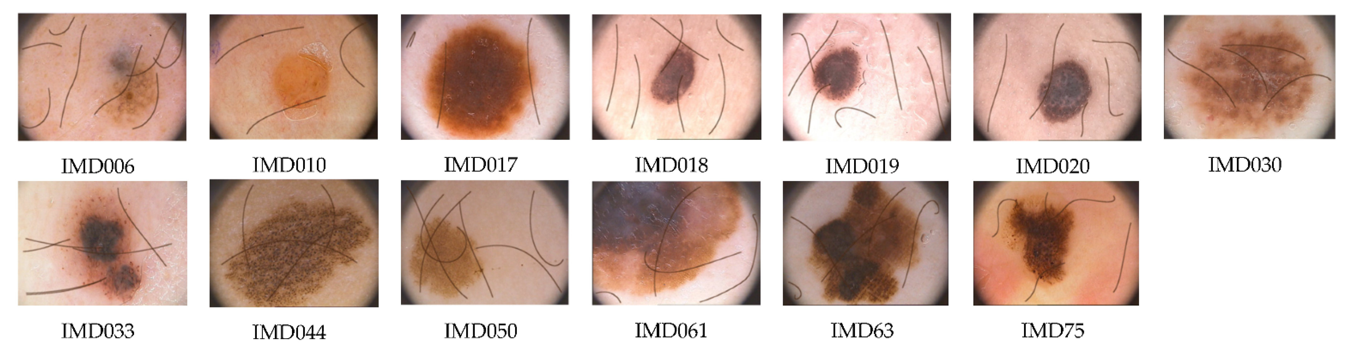
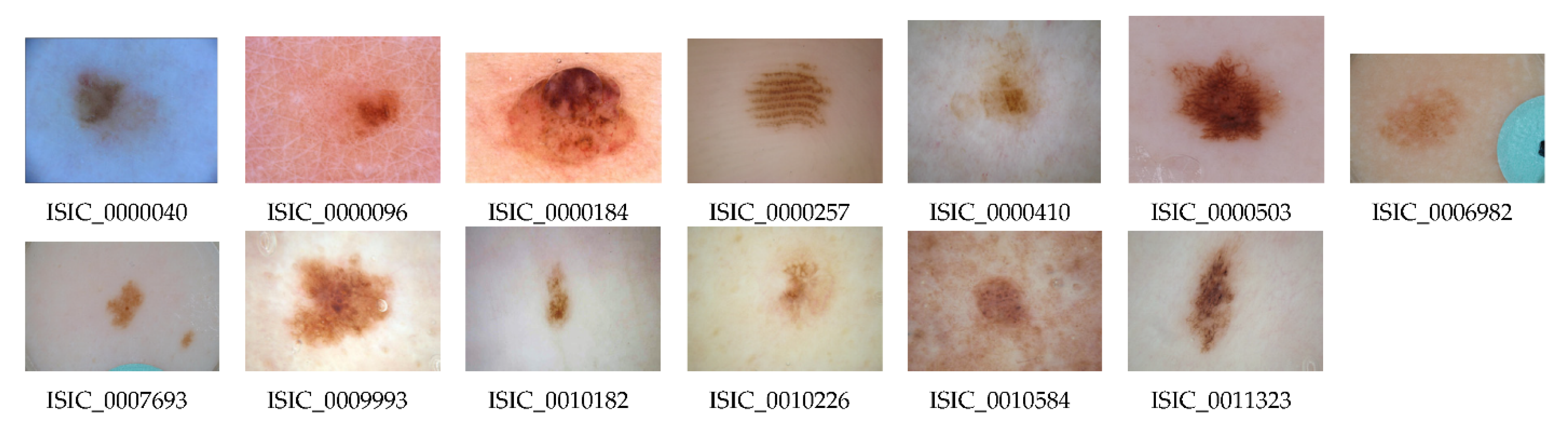
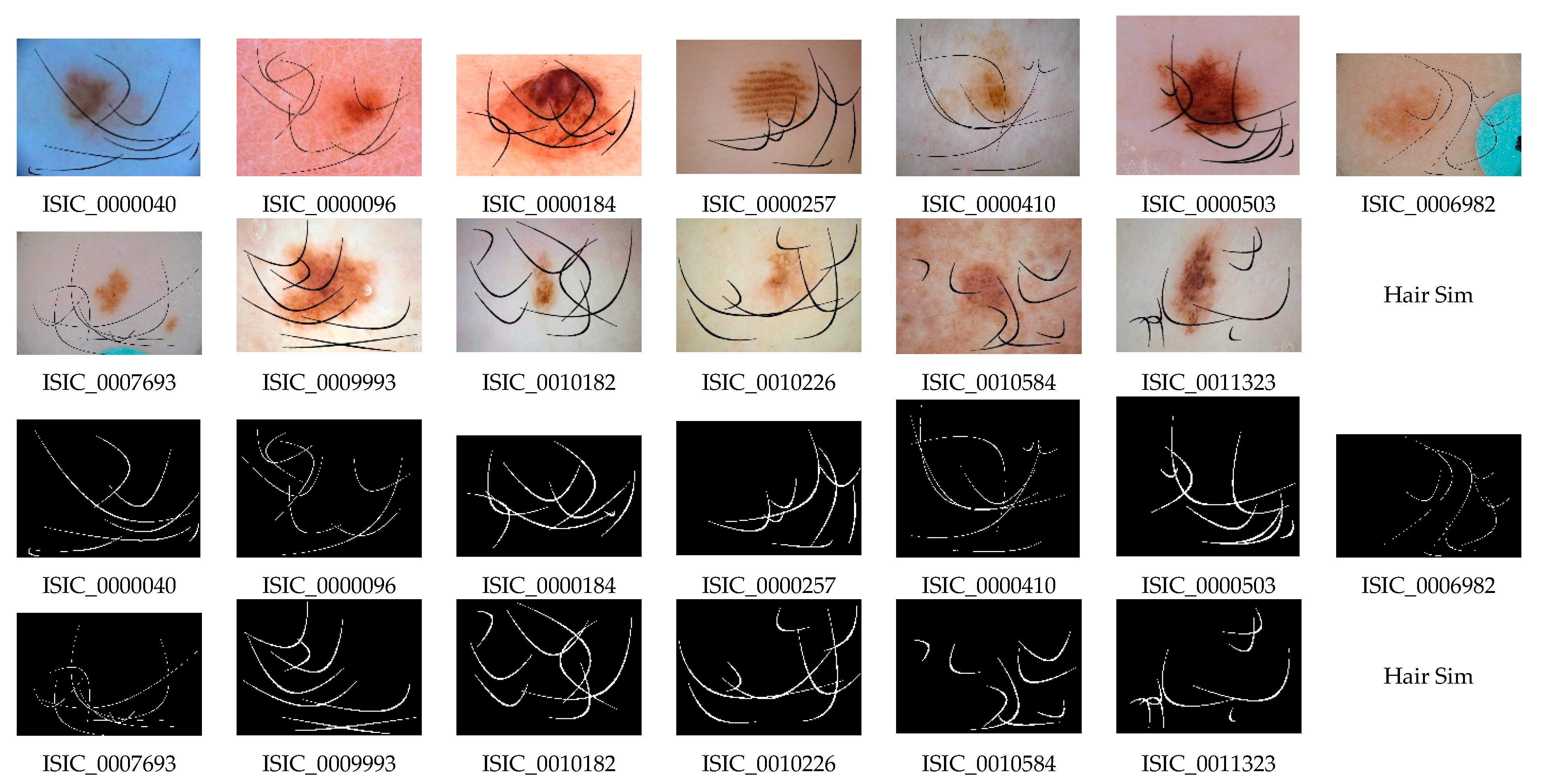
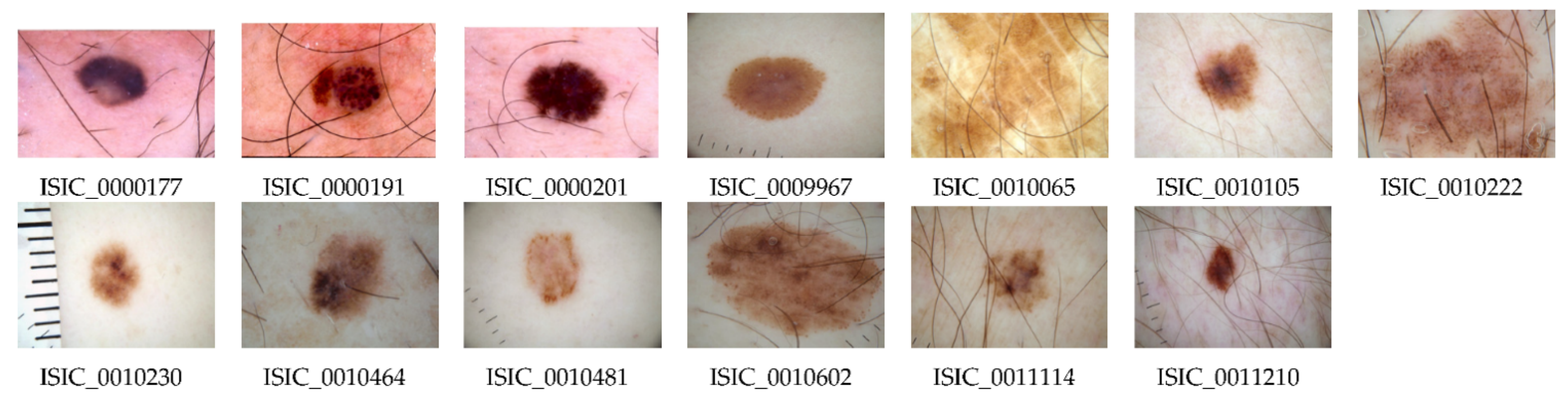
3.1. Datasets

We test our method by considering images available on two publicly available databases of dermoscopic images: PH² [28] and ISIC2016 [29]. PH² is a dermoscopic image database acquired at the Dermatology Service of Hospital Pedro Hispano to support comparative studies on segmentation/classification methods. This database includes clinical/histological diagnosis, medical annotation, and the evaluation of many dermoscopic criteria. It provides 200 dermoscopic RGB images and the corresponding ground truth, including 80 atypical nevi, 80 common nevi, and 40 melanomas. All the images are 8-bit RGB and have resolution 760 × 560 pixels. ISIC2016 is one of the largest databases of dermoscopic images of skin lesions with quality control held by the International Symposium on Biomedical Imaging (ISBI) to improve melanoma diagnosis. It includes images representative of both benign and malignant skin lesions. For each image, the ground truth is also available. ISIC2016 consists of 397 (75 melanomas) and 900 (173 melanomas) annotated images as testing and training data, respectively. The images are 8-bit RGB and have a size ranging from 542 × 718 to 2848 × 4288. PH² and ISIC2016 databases contain numerous images with complex backgrounds and complicated skin conditions with the presence of hair and other artifacts/aberrations.

Since in PH² and ISIC2016 hairless and hairy images are not distinguished, it is not possible to evaluate the performance of an HR method on each total dataset, and it is necessary to separate them preliminarily. Hence, from PH² and ISIC2016 we extract two datasets, denoted as H-data and NH-data, each constituted by 170 images, which respectively contain images with evident hair and images without hair. These images are selected randomly and subdivided into the two datasets according to a human visual inspection. These datasets, totally comprising 340 images, are available at the Github link indicated in the section Data Availability Statement.

To accurately and comprehensively validate the goodness of detecting hair and, at the same time, to make a deeper comparison with the published results of the existing methods [18,19,20,21,22,23], which in the following we indicate with the name of the first author (i.e., Lee, Xie, Huang, Abbas, Toossi, Bibiloni), we also consider a specific dataset available in [37]. This dataset, here call NH13-data and shown in Figure 4, is constituted by 13 images without hair. We consider also the hairy images obtained starting from NH13-data by the GAN method [38] and HairSim method [39], that starting from a hair-free dermoscopic image, provide a hair-occluded image and the corresponding binary hair-mask. These datasets are available in [37], are denoted as H13GAN-data and H13Sim-data, and are shown in Figure 5 and Figure 6, respectively.

Moreover, to validate the performance of the method on a larger dataset, we simulate the presence of hair on NH-data using the HairSim method by generating the HSim-data set. Note that for HSim-data and H-data, only the methods Lee, Xie, and HR-SSC are considered. The choice of these methods is based on the fact that first, they are the only methods, including the deep learning class of methods, with an available source code, second, they are used widely in the literature, and third, they have higher quality measures in [37]. We consider all images of H-data and HSim-data, but, given the high number of images, we limit to show the results for a13 images sample for each dataset, here named sH-data and sHSim-data, respectively. To favor the visual comparison of the results, the sNH-data from which sHSim-data are generated are shown in Figure 7, while in Figure 8 and Figure 9 sHSim-data and sH-data, together with the corresponding added hair, are respectively shown. Additionally, all of these datasets are available at the above Github link to support the possibility of comparison by other authors.

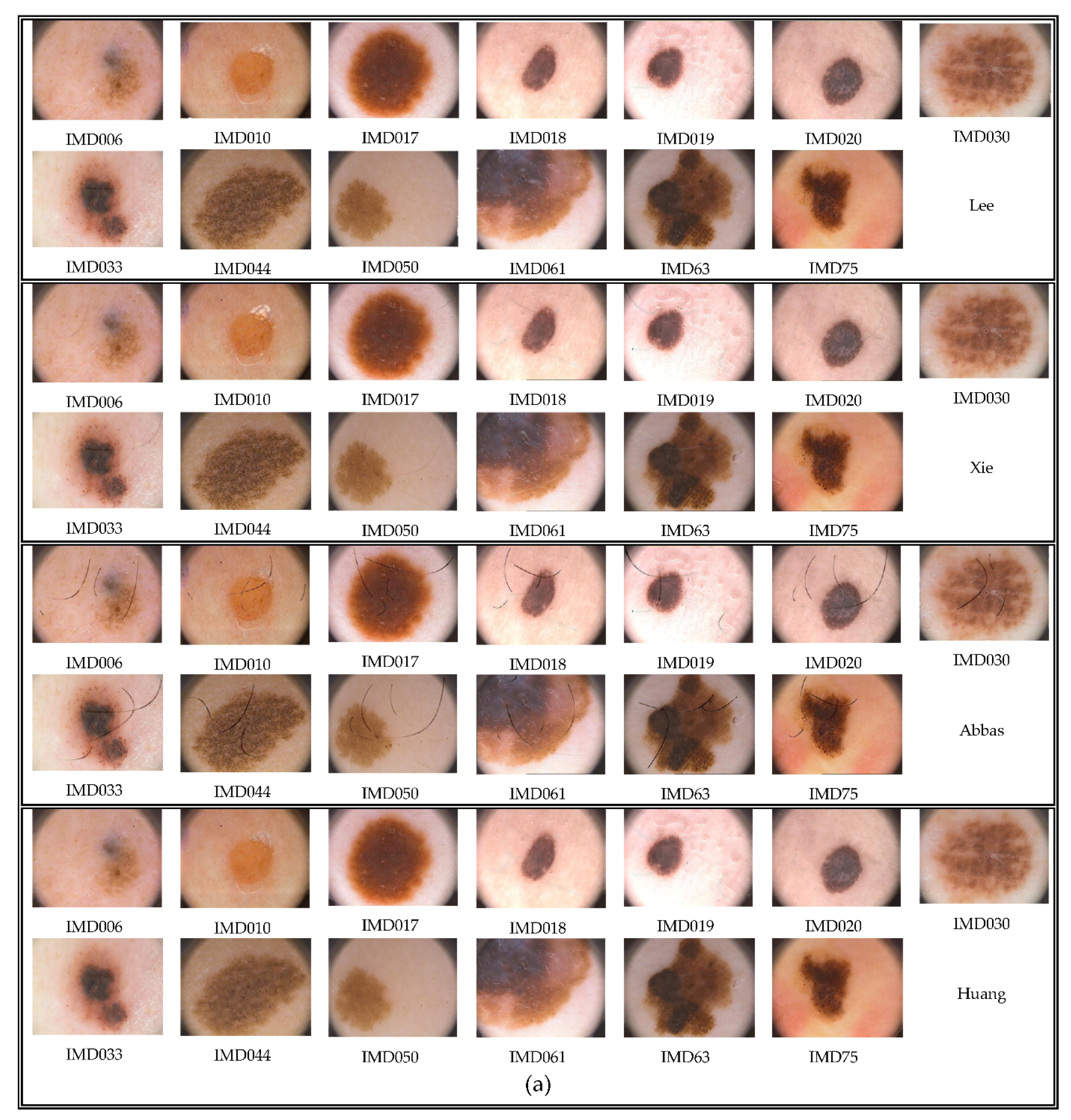
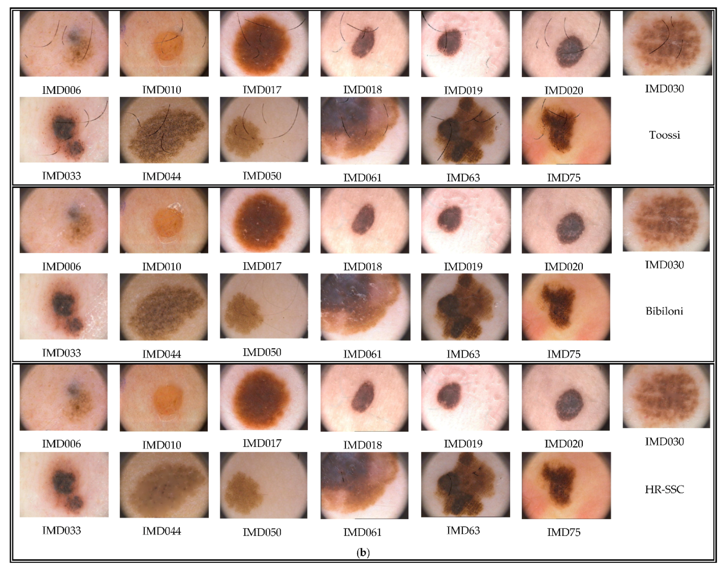
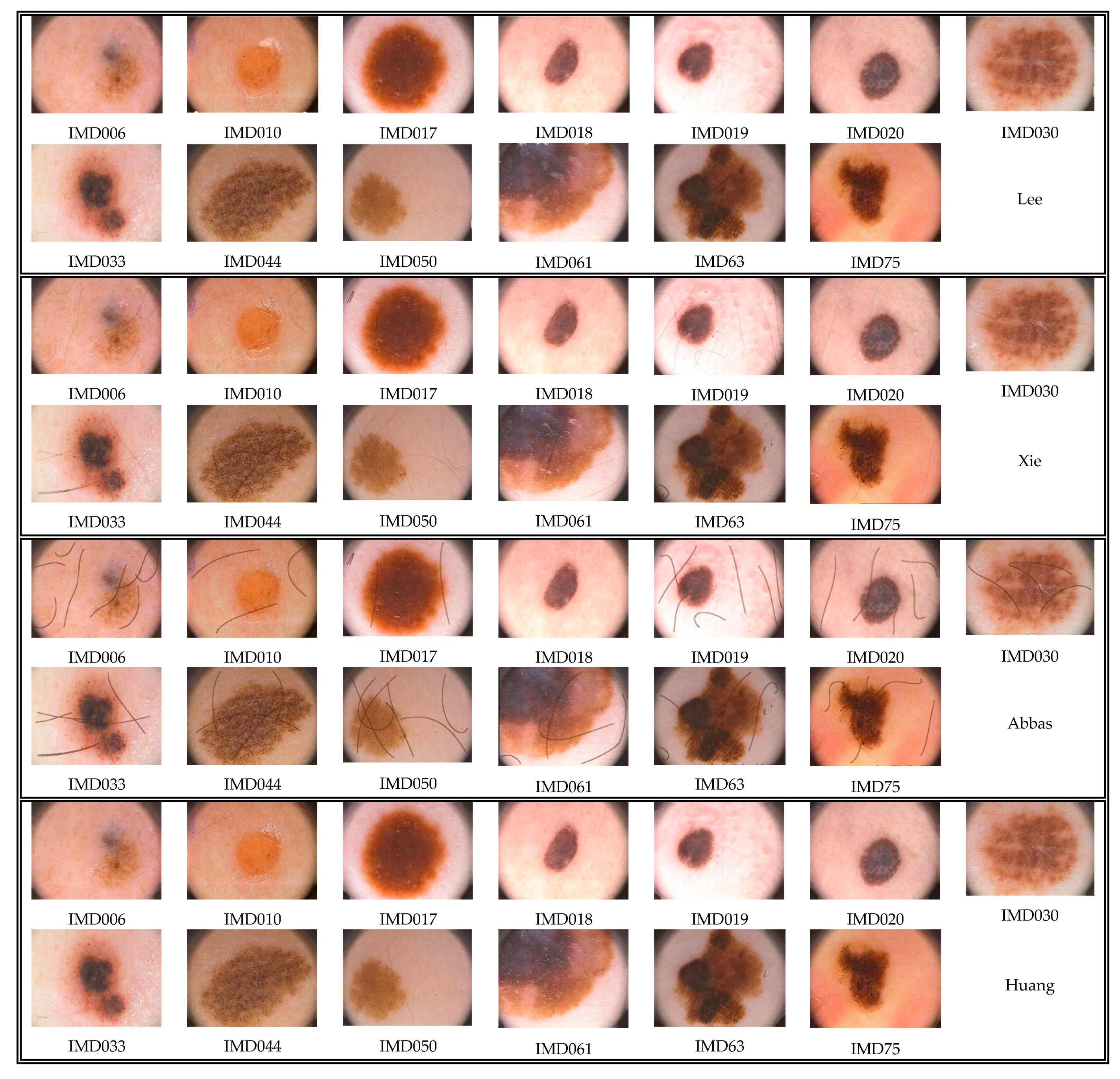
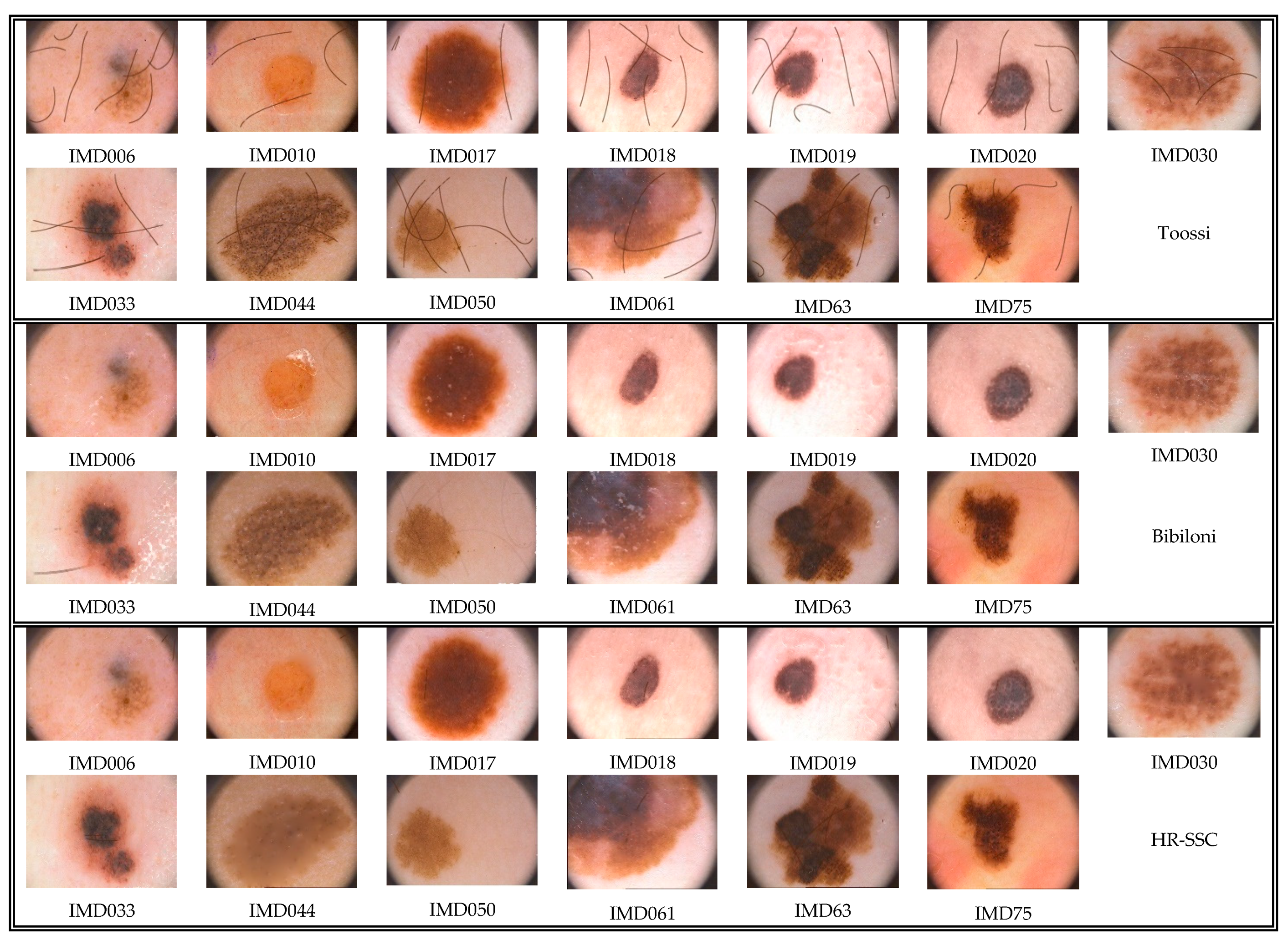
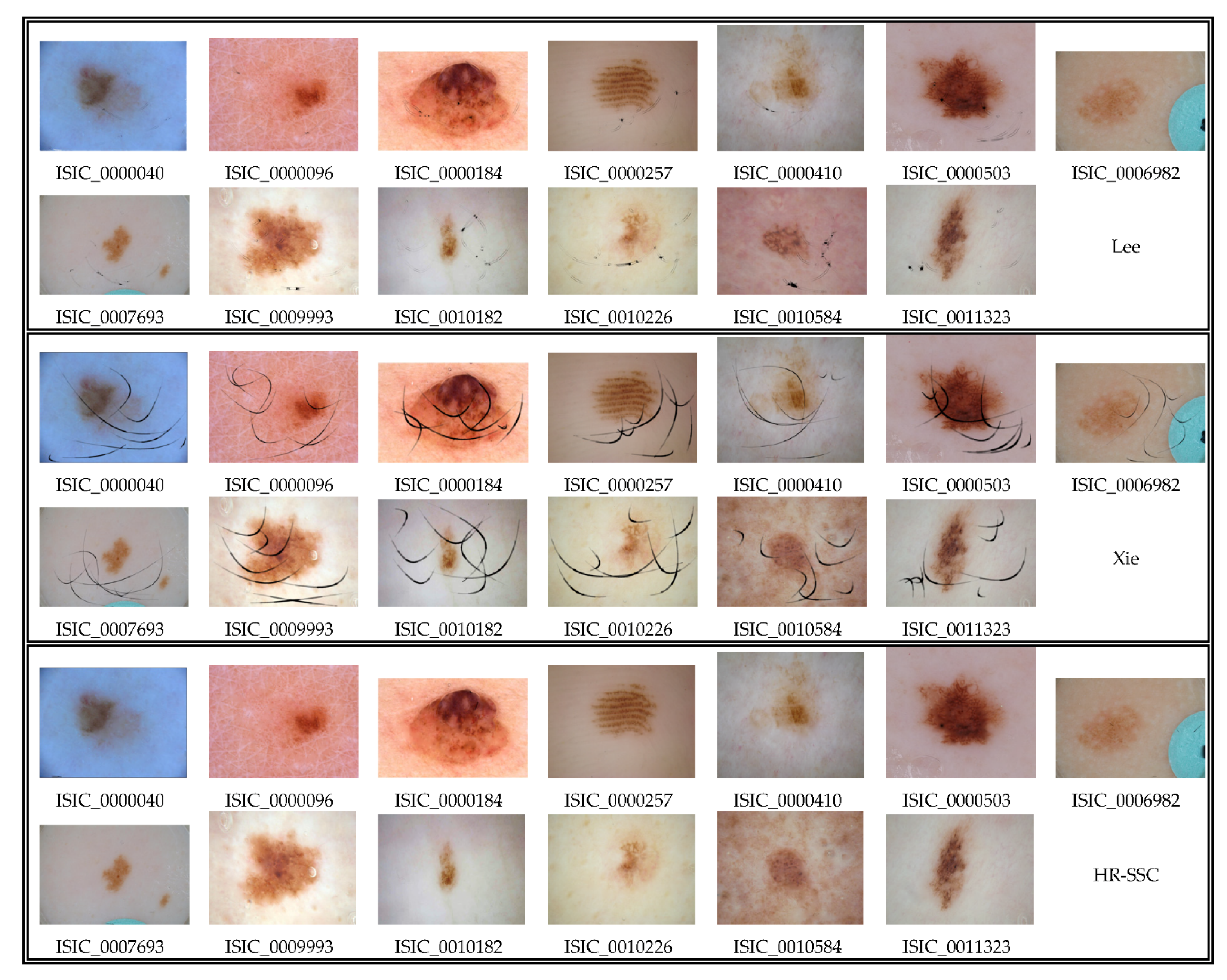
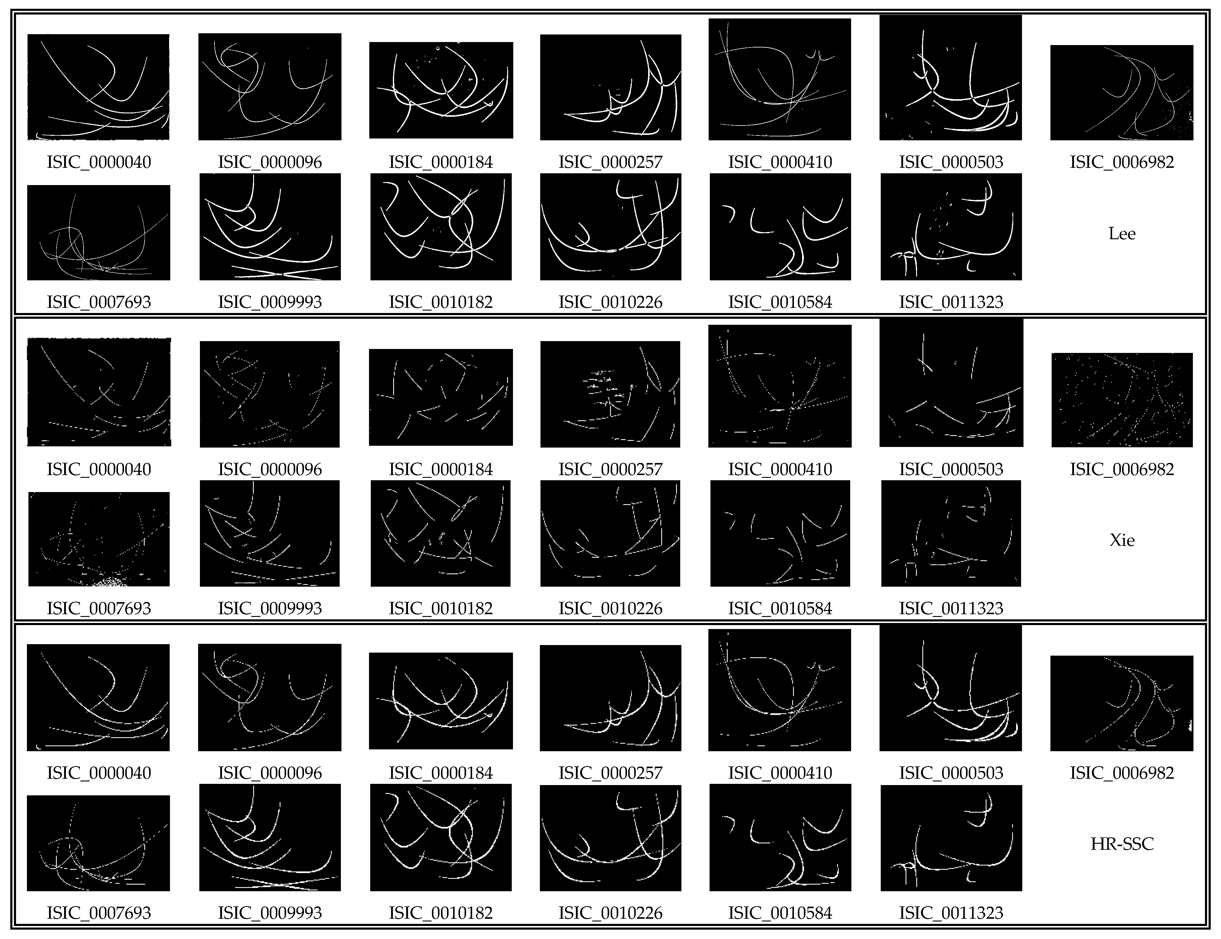
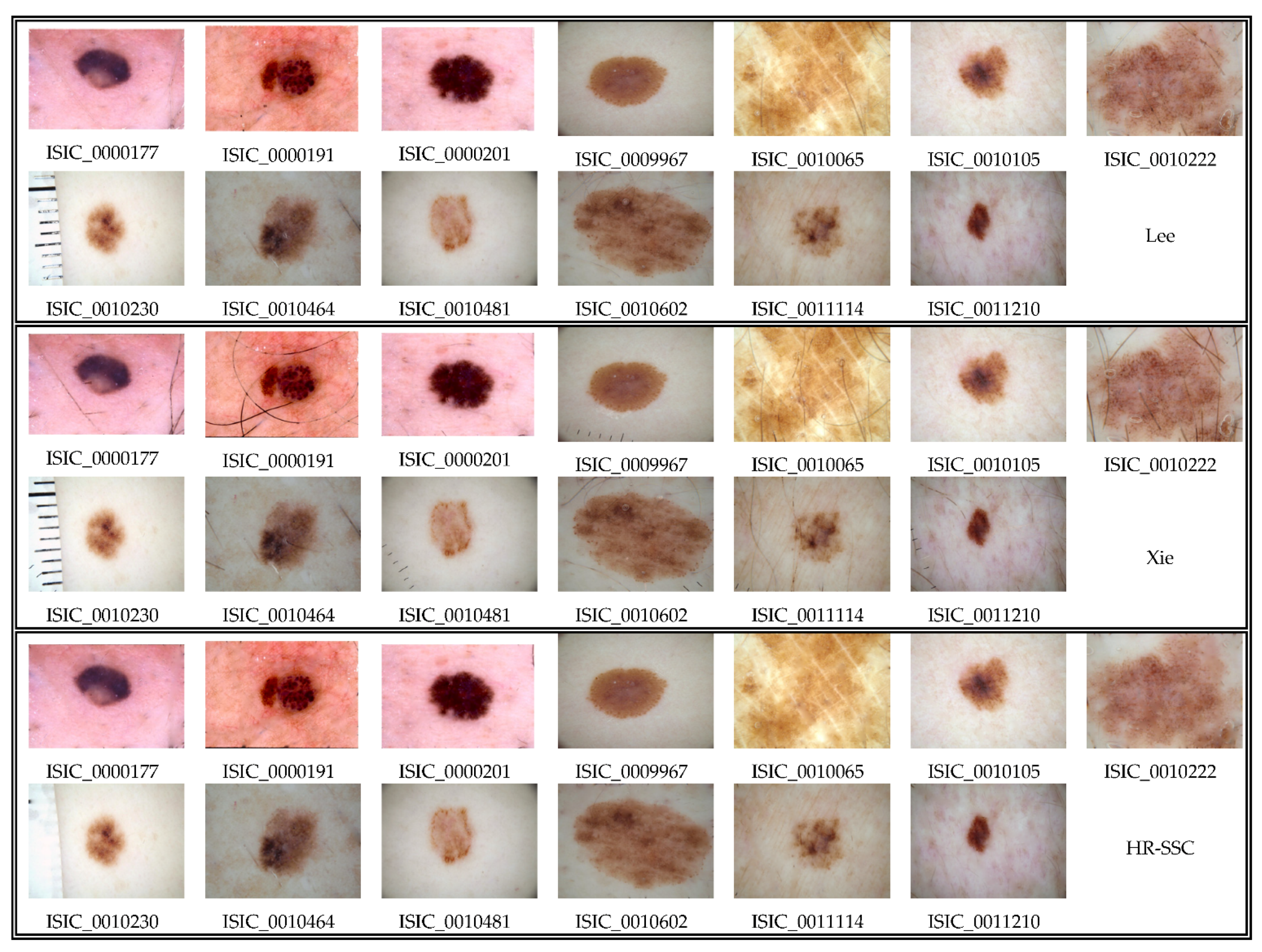
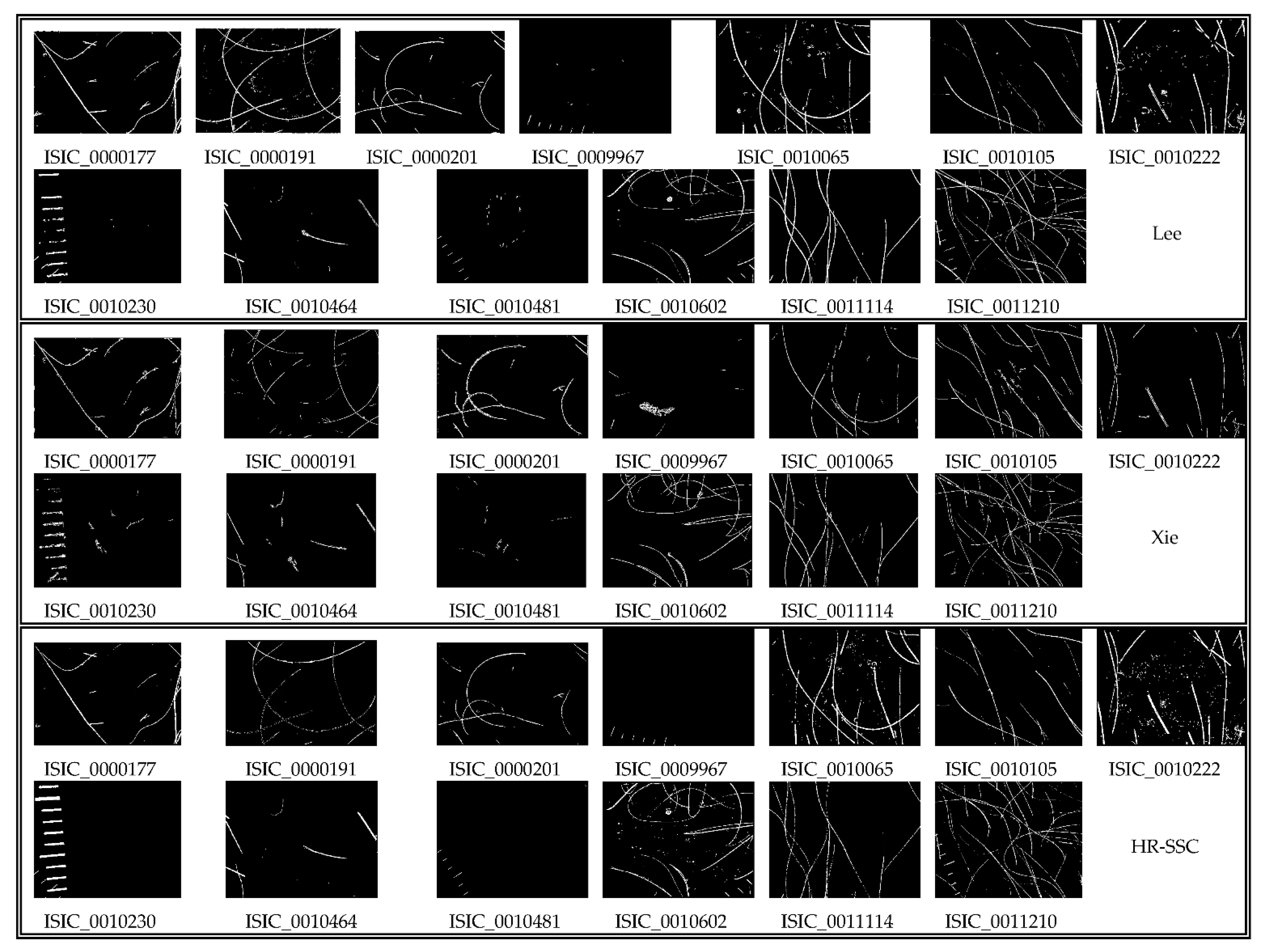
3.2. Qualitative Evaluation

To perform a qualitative evaluation, we check, for each method under consideration, if the set of images selected as hairy images by a method is (almost) equal to the corresponding original dataset, and we verify if the appearance of the inpainted image is good. For this purpose, we consider all the images (with and without hair) belonging to both H-data and NH-data, and we perform the following evaluations.

(a)

We check whether, in most cases, the hair determination is successful or not, i.e., that the images are re-confirmed as belonging to H-data and NH-data, respectively. This allows us to determine for the different considered methods how much the resulting sets belonging to H-data or NH-data are equal to the initial ones.

(b)

We verify if the appearance of the hairless resulting image is, according to human subjective judgment, compatible with a hairless and good quality version of it. Moreover, we test whether the presence of the hair can preclude or alter a subsequent step of skin lesion segmentation.

(c)

We visually compare the obtained results by the proposed method and those directly available in [37] or by the available implementation of Lee and Xie on H13GAN-data, H13Sim-data, HSim-data, and H-data to determine their overall performance.

In regard to the assessment of point (a), we find that the classification error is within 25%, 65%, 10%, respectively, for Lee, Xie, and HR-SSC. As concerns the assessment of point (b), the visual inspection of the results shows that the resulting perceptual quality is in accordance with the percentages obtained for point (a). To verify the effectiveness of the hair removal methods, a recent SLS method [14,15] is applied. The segmentation results show that hair removal applied before the segmentation process involves an improvement of about 70%, 20%, 90% for Lee, Xie, and HR-SSC, respectively. The results of the visual comparison on the various datasets of point (c) are given in Figure 10 and Figure 11 on H13GAN-data and H13Sim-data, respectively. To give major visual evidence and to facilitate the comparison, in Figure 12 and Figure 13, the results on sHSim-data and the corresponding final mask are respectively shown. The same is true for Figure 14 and Figure 15, where results on H-data with the corresponding final mask are shown.

In summary, in relation to the qualitative evaluation, from the visual examination of the resulting images of each method available in [37] and HR-SSC on H13GAN-data and H13Sim-data (see Figure 10 and Figure 11), it appears that evident hair regions are not detected by Abbas and Toossi. Limiting the comparison only to the three methods of Lee, Xie, and HR-SSC, evident hair regions are not detected by Xie on the HSim-data and, to a lesser extent, on H-data. See the results on the sample sHsim-data in Figure 12 and on the sample sH-data in Figure 14. Note that HR-SSC is able also to remove the ruler marks that can be mistaken as hair (see Figure 14 and Figure 15).

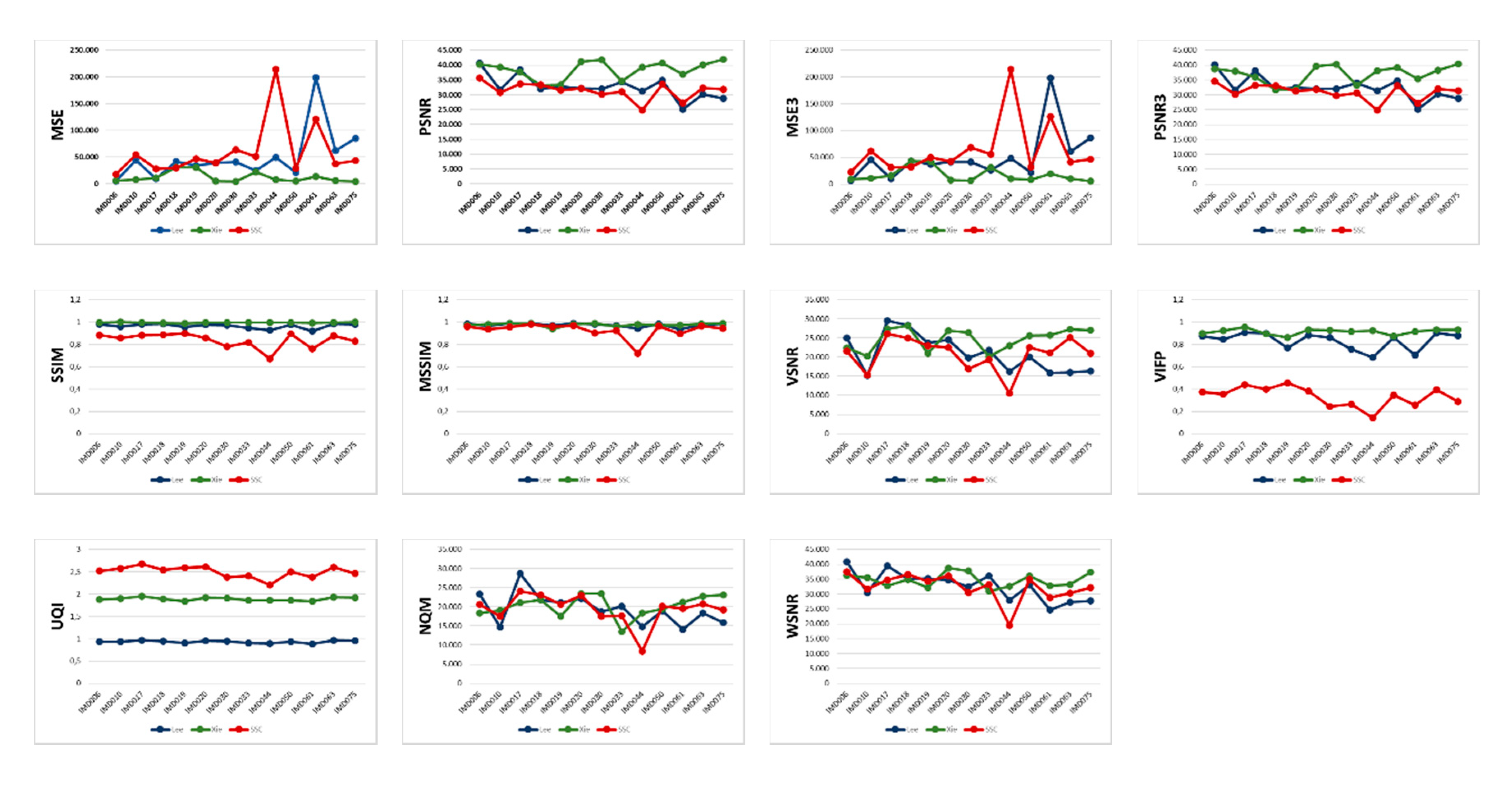
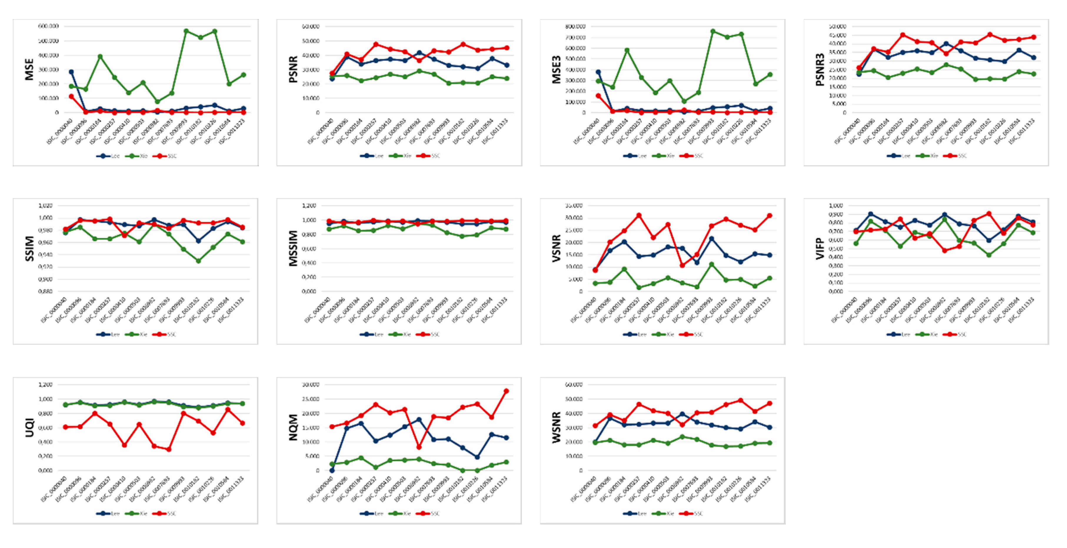
3.3. Quantitative Evaluation

We quantitatively evaluate the resulting images on the hairless image datasets to which hair has been added (see Section 3.1) by considering the original image as ground truth and expressing a quantitative evaluation in terms of the following:

-

nine most popular quality measures: MSE, PSNR, MSE3, PSNR3, SSIM, MSSIM, VSNR, VIFP, UQI, NQM, WSNR [40,41];

-

area of the detected hair regions;

-

true/false discovery rate (see the definition in Section 3.3.3).

Although the above quality measures are related to human perception to a small extent, and the problem to define adequate metrics for the performance evaluation of color image processing methods remains an open problem widely studied [41,42,43,44,45], most often, these measures are extensively employed to evaluate the performance of many types of image analysis methods, including the HR methods [17,37]. In turn, we see these quality measure values as valid indicators since they contribute to delineate the trend of the performance of an HR method, and, at the same time, we consider them not suitable alone to give evidence of its effectiveness. To overcome this gap, since the determination of the effective hair area and the true/false rate are the major critical points for the quantitative evaluation of HR methods, we extend the performance evaluation by measuring the hair area and true/false rate (see respective Section 3.3.2 and Section 3.3.3). As mentioned above, following [17,37], we consider the images in which, in a controlled way, the hair regions are introduced on input hair-free images by using suitable hair insertion methods [38,39] that provide a hair-occluded image and the corresponding binary hair mask. The resulting binary mask is used as ground truth to quantitatively evaluate the performance by computing the detected area and the false discovery rate/true discovery rate (FDR/TDR).

Note that we use the hairy images used in [17] and those available at [37]. Then, we extend the controlled hair simulation on a larger dataset, and to allow comparison with other HR methods on the same image dataset, we made it available at the already mentioned Github link. Indeed, currently, the direct comparison with the results shown in another paper is in practice impossible since the experimental results are given for a not well-specified dataset. Accordingly, we think that having a shared dataset with the corresponding ground truth is a useful tool favoring the comparison and increasing the quality of the performance evaluation.

3.3.1. Quantitative Evaluation Based on Quality Measures

To carry out a quantitative evaluation based on quality measures, we consider the results obtained by all methods (see Figure 10 and Figure 11) on the image datasets H13Sim-data and H13Sim-data (see Figure 5 and Figure 6), and we compute the metric values by considering the original images in NH13-data as ground truths (see Figure 4). The metric values are shown in

Table 1. Quality evaluation of the results on the H13GAN-data—best results are in bold.

Img	Met.	MSE	PSNR	MSE3	PSNR3	SSIM	MSSIM	VSNR	VIFP	UQI	NQM	WSNR
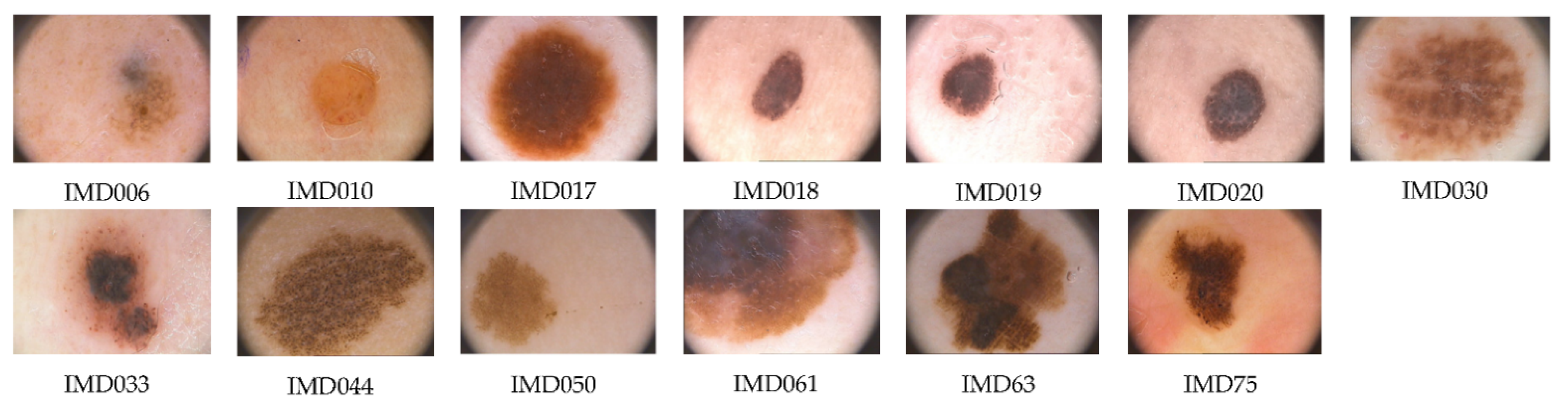
IMD006	Lee	13.626	36.787	20.918	34.926	0.888	0.956	24.401	0.403	0.650	23.151	40.255
	Xie	12.610	37.124	19.831	35.157	0.891	0.957	25.355	0.412	0.653	22.687	40.286
	Abbas	57.555	30.530	64.073	30.064	0.856	0.898	15.260	0.354	0.608	12.372	28.927
	Huang	24.283	34.278	33.481	32.883	0.860	0.926	19.601	0.301	0.534	16.305	33.955
	Toossi	55.748	30.668	62.440	30.176	0.853	0.897	15.370	0.342	0.591	12.586	29.143
	Bibiloni	19.653	35.197	28.070	33.648	0.867	0.943	21.588	0.328	0.589	19.411	36.740
	HR-SSC	19.669	35.193	27.078	33.805	0.861	0.941	21.101	0.323	0.561	20.950	37.581
IMD010	Lee	44.373	31.660	52.734	30.910	0.855	0.939	16.990	0.352	0.659	18.189	33.261
	Xie	46.305	31.475	55.898	30.657	0.859	0.931	15.853	0.364	0.665	14.288	30.576
	Abbas	88.070	28.683	98.376	28.202	0.838	0.907	14.944	0.330	0.636	14.129	28.725
	Huang	42.985	31.798	52.674	30.915	0.818	0.905	17.330	0.236	0.510	17.169	32.186
	Toossi	90.161	28.581	100.956	28.089	0.832	0.905	15.007	0.320	0.618	13.841	28.495
	Bibiloni	40.550	32.051	51.019	31.054	0.857	0.937	16.699	0.354	0.660	16.755	32.390
	HR-SSC	55.952	30.653	66.185	29.923	0.827	0.920	15.203	0.293	0.579	17.837	31.972
IMD017	Lee	18.625	35.430	24.645	34.213	0.881	0.957	29.130	0.445	0.711	27.359	38.837
	Xie	16.228	36.028	22.790	34.553	0.884	0.955	30.411	0.455	0.714	25.465	38.191
	Abbas	61.528	30.240	67.983	29.807	0.847	0.911	21.698	0.390	0.662	17.373	28.555
	Huang	29.318	33.459	35.611	32.615	0.854	0.937	25.118	0.366	0.601	20.446	32.682
	Toossi	62.801	30.151	68.982	29.743	0.840	0.907	21.591	0.374	0.636	17.371	28.516
	Bibiloni	24.312	34.273	30.787	33.247	0.867	0.948	26.935	0.406	0.684	23.497	35.660
	HR-SSC	31.007	33.216	36.943	32.455	0.850	0.934	25.550	0.371	0.632	23.808	34.512
IMD018	Lee	53.072	30.882	58.624	30.450	0.865	0.960	27.433	0.353	0.581	22.039	35.006
	Xie	18.253	35.517	23.648	34.393	0.863	0.956	28.108	0.352	0.578	25.368	40.353
	Abbas	112.129	27.634	117.432	27.433	0.850	0.913	17.475	0.344	0.570	14.966	28.474
	Huang	65.664	29.958	71.773	29.571	0.845	0.939	22.471	0.286	0.476	18.580	32.252
	Toossi	108.744	27.767	113.634	27.576	0.849	0.915	17.689	0.340	0.563	15.181	28.639
	Bibiloni	54.371	30.777	60.419	30.319	0.861	0.957	26.734	0.343	0.574	21.670	34.753
	HR-SSC	34.432	32.761	39.240	32.194	0.853	0.955	24.135	0.327	0.537	22.638	36.055
IMD019	Lee	40.674	32.038	49.993	31.142	0.882	0.942	24.415	0.414	0.696	21.020	35.377
	Xie	41.599	31.940	51.373	31.023	0.886	0.938	24.315	0.427	0.700	19.620	34.346
	Abbas	80.579	29.069	90.699	28.555	0.856	0.908	18.686	0.372	0.657	16.024	30.163
	Huang	60.703	30.299	71.582	29.583	0.827	0.904	20.229	0.273	0.507	18.011	32.313
	Toossi	81.503	29.019	91.594	28.512	0.846	0.904	18.662	0.355	0.634	16.105	30.222
	Bibiloni	49.196	31.212	59.452	30.389	0.868	0.934	23.136	0.375	0.672	19.580	34.043
	HR-SSC	56.414	30.617	65.961	29.938	0.858	0.930	21.562	0.363	0.642	18.991	33.110
IMD020	Lee	54.462	30.770	61.126	30.269	0.842	0.958	23.801	0.362	0.653	22.282	34.661
	Xie	23.642	34.394	29.561	33.424	0.846	0.957	26.239	0.373	0.660	25.905	40.384
	Abbas	132.080	26.922	138.996	26.701	0.803	0.883	15.764	0.306	0.604	14.074	26.834
	Huang	62.554	30.168	69.851	29.689	0.815	0.936	21.317	0.303	0.564	19.108	32.275
	Toossi	125.759	27.135	132.544	26.907	0.796	0.884	16.111	0.295	0.581	14.456	27.197
	Bibiloni	59.850	30.360	67.234	29.855	0.828	0.951	22.518	0.329	0.630	20.985	33.649
	HR-SSC	43.098	31.786	48.657	31.259	0.817	0.949	22.203	0.316	0.590	23.641	36.222
IMD030	Lee	50.827	31.070	57.665	30.522	0.864	0.952	19.959	0.398	0.660	18.341	32.244
	Xie	16.425	35.976	23.671	34.389	0.869	0.959	26.493	0.413	0.669	25.476	39.857
	Abbas	70.112	29.673	76.885	29.272	0.838	0.917	18.528	0.352	0.623	15.447	29.300
	Huang	50.556	31.093	57.620	30.525	0.847	0.941	20.743	0.347	0.599	19.632	32.935
	Toossi	72.517	29.526	79.211	29.143	0.830	0.912	18.330	0.337	0.600	15.616	29.428
	Bibiloni	45.920	31.511	53.062	30.883	0.855	0.949	21.692	0.372	0.647	19.680	33.360
	HR-SSC	59.202	30.407	66.783	29.884	0.786	0.904	17.204	0.252	0.468	19.009	31.509
IMD033	Lee	29.071	33.496	36.028	32.564	0.858	0.948	23.146	0.348	0.623	20.946	37.195
	Xie	20.680	34.975	27.696	33.707	0.874	0.954	26.280	0.389	0.646	20.928	38.139
	Abbas	87.505	28.710	94.489	28.377	0.825	0.894	16.762	0.302	0.574	12.081	28.385
	Huang	33.270	32.910	40.516	32.055	0.836	0.926	21.584	0.280	0.523	18.372	34.461
	Toossi	86.218	28.775	93.278	28.433	0.815	0.890	16.783	0.286	0.547	12.324	28.584
	Bibiloni	38.722	32.251	45.577	31.543	0.839	0.932	20.980	0.296	0.588	18.178	34.092
	HR-SSC	56.659	30.598	64.342	30.046	0.785	0.894	18.590	0.207	0.451	16.917	32.624
IMD044	Lee	47.457	31.368	53.355	30.859	0.863	0.943	17.641	0.421	0.738	16.903	29.594
	Xie	18.590	35.438	27.085	33.804	0.887	0.964	25.971	0.494	0.774	23.188	36.594
	Abbas	72.923	29.502	78.288	29.194	0.867	0.926	16.276	0.457	0.750	12.369	25.924
	Huang	105.875	27.883	110.178	27.710	0.745	0.835	12.993	0.210	0.484	12.174	23.933
	Toossi	73.452	29.471	78.674	29.172	0.859	0.923	16.110	0.440	0.736	12.445	25.910
	Bibiloni	96.722	28.276	101.895	28.049	0.763	0.867	13.711	0.242	0.561	13.030	24.693
	HR-SSC	176.341	25.667	179.590	25.588	0.673	0.734	11.356	0.143	0.345	9.157	20.718
IMD050	Lee	35.787	32.594	41.721	31.927	0.880	0.954	18.895	0.335	0.578	17.676	31.938
	Xie	22.695	34.572	28.814	33.535	0.881	0.953	22.280	0.337	0.578	19.716	34.639
	Abbas	49.806	31.158	55.624	30.678	0.859	0.898	18.094	0.314	0.554	12.763	28.703
	Huang	22.682	34.574	29.144	33.485	0.852	0.932	22.328	0.232	0.453	18.434	34.242
	Toossi	49.658	31.171	55.452	30.692	0.856	0.897	18.151	0.300	0.536	12.899	28.805
	Bibiloni	24.683	34.207	30.624	33.270	0.876	0.949	20.898	0.335	0.575	19.338	33.924
	HR-SSC	32.032	33.075	38.428	32.284	0.863	0.944	21.815	0.269	0.507	19.705	34.589
IMD061	Lee	200.137	25.118	206.683	24.978	0.818	0.913	16.492	0.340	0.655	14.269	24.901
	Xie	31.045	33.211	39.240	32.194	0.853	0.947	28.493	0.401	0.701	24.189	35.438
	Abbas	162.905	26.011	170.740	25.807	0.774	0.862	19.898	0.262	0.585	17.621	27.216
	Huang	118.122	27.408	125.806	27.134	0.824	0.930	19.472	0.341	0.641	18.026	28.664
	Toossi	160.195	26.084	168.469	25.866	0.759	0.856	19.691	0.248	0.552	17.752	27.250
	Bibiloni	132.368	26.913	139.485	26.686	0.816	0.918	18.707	0.319	0.651	15.911	26.804
	HR-SSC	123.964	27.198	132.643	26.904	0.730	0.877	21.104	0.222	0.459	19.312	28.617
IMD063	Lee	73.087	29.492	78.056	29.207	0.868	0.949	16.458	0.395	0.638	18.376	27.193
	Xie	15.333	36.274	23.189	34.478	0.871	0.955	30.726	0.405	0.644	27.486	38.241
	Abbas	75.404	29.357	82.451	28.969	0.849	0.914	19.238	0.372	0.619	16.239	25.970
	Huang	82.506	28.966	87.606	28.705	0.846	0.931	15.781	0.328	0.563	16.786	25.992
	Toossi	74.619	29.402	81.598	29.014	0.847	0.914	19.316	0.364	0.608	16.268	25.989
	Bibiloni	74.387	29.416	80.223	29.088	0.861	0.948	16.314	0.374	0.626	18.402	27.149
	HR-SSC	38.011	32.332	44.806	31.617	0.852	0.945	25.076	0.355	0.586	21.399	30.795
IMD075	Lee	98.538	28.195	107.530	27.816	0.860	0.948	16.524	0.354	0.624	15.793	27.594
	Xie	18.342	35.496	29.230	33.473	0.866	0.952	26.945	0.373	0.635	24.586	38.198
	Abbas	73.194	29.486	82.107	28.987	0.845	0.926	18.078	0.336	0.606	16.732	28.717
	Huang	112.433	27.622	122.341	27.255	0.821	0.917	15.514	0.251	0.486	14.620	26.485
	Toossi	71.889	29.564	80.600	29.067	0.841	0.926	18.156	0.325	0.590	16.955	28.867
	Bibiloni	93.923	28.403	103.663	27.975	0.855	0.948	17.089	0.344	0.618	15.988	27.807
	HR-SSC	45.132	31.586	53.234	30.869	0.814	0.925	20.687	0.256	0.491	19.150	31.981

and

Table 2. Quality evaluation of the results on the H13Sim-data—best results are in bold.

Img	Met.	MSE	PSNR	MSE3	PSNR3	SSIM	MSSIM	VSNR	VIFP	UQI	NQM	WSNR
IMD006	Lee	5.443	40.773	6.400	40.069	0.978	0.985	25.044	0.873	0.938	23.320	40.853
	Xie	6.105	40.274	8.712	38.730	0.998	0.971	22.402	0.898	0.944	18.362	36.300
	Abbas	146.175	26.482	149.923	26.372	0.920	0.836	9.709	0.747	0.877	6.777	23.447
	Huang	14.654	36.471	17.000	35.826	0.964	0.971	20.263	0.817	0.905	16.575	34.655
	Toossi	147.390	26.446	151.565	26.325	0.913	0.831	9.707	0.715	0.857	6.726	23.421
	Bibiloni	14.087	36.642	19.991	35.123	0.937	0.960	21.615	0.536	0.830	18.990	36.561
	HR-SSC	17.983	35.582	22.252	34.657	0.882	0.961	21.630	0.373	0.637	20.652	37.497
IMD010	Lee	44.462	31.651	45.490	31.552	0.960	0.969	15.108	0.844	0.935	14.718	30.440
	Xie	7.632	39.304	10.396	37.962	0.999	0.979	20.231	0.924	0.967	19.061	35.559
	Abbas	93.505	28.422	96.605	28.281	0.935	0.894	12.548	0.769	0.904	10.231	25.941
	Huang	21.230	34.861	22.192	34.669	0.962	0.967	20.111	0.819	0.919	17.995	33.880
	Toossi	94.868	28.360	99.195	28.166	0.926	0.889	12.520	0.734	0.882	10.253	25.956
	Bibiloni	49.427	31.191	55.047	30.723	0.973	0.971	16.917	0.850	0.953	14.449	30.158
	HR-SSC	54.625	30.757	61.890	30.215	0.856	0.937	15.234	0.353	0.666	17.575	31.736
IMD017	Lee	9.535	38.338	9.855	38.194	0.981	0.988	29.519	0.905	0.967	28.643	39.534
	Xie	11.082	37.684	16.277	36.015	0.997	0.986	27.386	0.955	0.979	21.083	32.729
	Abbas	64.666	30.024	67.694	29.825	0.941	0.934	20.432	0.758	0.902	15.536	26.897
	Huang	13.747	36.749	14.357	36.560	0.978	0.986	26.004	0.896	0.944	21.100	33.753
	Toossi	66.238	29.920	69.393	29.718	0.930	0.928	20.432	0.714	0.871	15.469	26.880
	Bibiloni	17.438	35.716	19.820	35.160	0.950	0.972	26.695	0.648	0.904	23.420	35.196
	HR-SSC	28.231	33.624	31.105	33.202	0.881	0.954	26.097	0.437	0.727	24.092	34.710
IMD018	Lee	41.735	31.926	42.896	31.807	0.982	0.988	28.284	0.899	0.944	21.864	34.994
	Xie	31.009	33.216	43.166	31.779	0.993	0.987	28.252	0.895	0.942	21.820	34.947
	Abbas	43.583	31.738	44.880	31.610	0.972	0.983	27.268	0.829	0.921	21.782	34.845
	Huang	41.980	31.900	43.166	31.779	0.981	0.987	28.252	0.895	0.942	21.820	34.947
	Toossi	246.045	24.221	251.091	24.132	0.936	0.831	11.292	0.841	0.911	9.424	23.138
	Bibiloni	44.101	31.686	45.648	31.537	0.972	0.983	27.226	0.792	0.930	21.523	34.748
	HR-SSC	29.831	33.384	31.740	33.115	0.886	0.978	25.032	0.396	0.652	23.172	36.610
IMD019	Lee	34.227	32.787	37.125	32.434	0.954	0.968	23.690	0.770	0.908	21.101	35.203
	Xie	30.434	33.297	42.538	31.843	0.986	0.939	21.001	0.863	0.930	17.517	32.120
	Abbas	311.608	23.195	326.342	22.994	0.888	0.797	10.687	0.636	0.835	8.627	22.541
	Huang	44.906	31.608	47.752	31.341	0.945	0.960	20.896	0.739	0.874	17.755	32.540
	Toossi	314.691	23.152	330.173	22.943	0.873	0.790	10.693	0.587	0.799	8.581	22.515
	Bibiloni	51.861	30.982	56.227	30.631	0.921	0.946	21.807	0.561	0.846	18.834	32.594
	HR-SSC	46.419	31.464	49.458	31.188	0.897	0.960	22.956	0.454	0.754	20.611	34.265
IMD020	Lee	39.130	32.206	41.418	31.959	0.974	0.988	24.516	0.883	0.951	22.135	34.724
	Xie	5.025	41.120	7.099	39.619	0.998	0.981	26.952	0.933	0.965	23.517	38.794
	Abbas	151.333	26.331	157.032	26.171	0.919	0.864	13.518	0.709	0.879	11.620	24.574
	Huang	40.210	32.087	42.343	31.863	0.976	0.986	23.483	0.900	0.947	19.376	32.999
	Toossi	157.470	26.159	163.807	25.987	0.905	0.859	13.468	0.661	0.848	11.482	24.465
	Bibiloni	46.316	31.474	49.423	31.192	0.956	0.978	22.775	0.695	0.922	20.401	33.376
	HR-SSC	39.242	32.193	41.779	31.921	0.857	0.967	22.515	0.383	0.693	22.956	36.159
IMD030	Lee	40.468	32.060	40.968	32.006	0.970	0.979	19.777	0.861	0.945	18.713	32.452
	Xie	4.286	41.810	6.163	40.233	0.998	0.987	26.467	0.927	0.969	23.432	37.889
	Abbas	81.085	29.041	83.086	28.936	0.938	0.915	16.712	0.743	0.897	12.585	26.889
	Huang	36.536	32.504	36.838	32.468	0.982	0.986	21.820	0.911	0.960	20.087	33.643
	Toossi	84.981	28.838	87.182	28.727	0.925	0.908	16.518	0.697	0.867	12.657	26.939
	Bibiloni	36.763	32.477	39.569	32.157	0.954	0.971	21.777	0.675	0.913	19.905	33.500
	HR-SSC	63.601	30.096	68.802	29.755	0.782	0.901	16.937	0.245	0.462	17.583	30.554
IMD033	Lee	24.454	34.247	26.046	33.973	0.947	0.968	21.830	0.757	0.907	20.112	36.196
	Xie	22.402	34.628	31.323	33.172	0.995	0.958	20.109	0.915	0.952	13.498	30.916
	Abbas	189.799	25.348	194.689	25.237	0.901	0.855	12.471	0.662	0.853	6.665	23.295
	Huang	18.819	35.385	19.675	35.192	0.956	0.966	22.401	0.828	0.918	18.761	35.305
	Toossi	169.486	25.839	174.635	25.709	0.890	0.852	12.952	0.624	0.823	7.391	23.923
	Bibiloni	69.269	29.725	73.560	29.464	0.902	0.910	16.689	0.466	0.815	11.935	28.549
	HR-SSC	50.811	31.071	55.613	30.679	0.816	0.921	19.280	0.264	0.552	17.666	33.302
IMD044	Lee	49.270	31.205	47.786	31.338	0.927	0.943	16.197	0.684	0.890	14.864	27.824
	Xie	7.508	39.376	10.183	38.052	0.998	0.980	23.052	0.924	0.973	18.344	32.600
	Abbas	39.651	32.148	39.209	32.197	0.955	0.945	17.653	0.790	0.934	13.447	27.293
	Huang	73.354	29.477	71.510	29.587	0.891	0.901	14.120	0.594	0.813	12.372	25.252
	Toossi	44.653	31.632	44.317	31.665	0.941	0.938	17.253	0.734	0.911	13.250	26.963
	Bibiloni	124.034	27.195	127.439	27.078	0.764	0.829	12.416	0.221	0.562	11.719	22.787
	HR-SSC	214.183	24.823	214.147	24.824	0.671	0.718	10.498	0.142	0.342	8.445	19.567
IMD050	Lee	21.355	34.836	21.807	34.745	0.976	0.984	20.082	0.860	0.930	19.013	33.138
	Xie	5.561	40.680	7.855	39.179	0.998	0.970	25.606	0.874	0.934	19.433	36.204
	Abbas	121.210	27.295	122.357	27.255	0.930	0.838	12.242	0.790	0.895	7.594	23.528
	Huang	10.580	37.886	11.262	37.615	0.965	0.979	23.658	0.821	0.915	19.415	35.929
	Toossi	120.022	27.338	121.174	27.297	0.927	0.837	12.359	0.769	0.886	7.647	23.580
	Bibiloni	37.044	32.444	40.803	32.024	0.969	0.971	18.740	0.817	0.920	16.150	30.032
	HR-SSC	28.878	33.525	32.355	33.031	0.893	0.964	22.466	0.344	0.632	20.099	34.948
IMD061	Lee	199.214	25.138	197.816	25.168	0.918	0.934	15.841	0.705	0.881	14.097	24.753
	Xie	13.371	36.869	18.984	35.347	0.994	0.973	25.671	0.915	0.962	21.197	32.801
	Abbas	231.503	24.485	238.370	24.358	0.869	0.848	17.243	0.568	0.811	12.035	22.788
	Huang	92.491	28.470	92.932	28.449	0.965	0.979	19.645	0.871	0.939	17.979	28.910
	Toossi	230.406	24.506	237.676	24.371	0.853	0.839	17.117	0.526	0.778	11.960	22.729
	Bibiloni	125.200	27.155	127.409	27.079	0.919	0.937	18.203	0.551	0.875	15.407	26.464
	HR-SSC	120.609	27.317	126.001	27.127	0.760	0.895	21.122	0.254	0.535	19.579	28.808
IMD063	Lee	62.239	30.190	60.750	30.295	0.984	0.977	16.040	0.902	0.959	18.381	27.253
	Xie	6.407	40.064	9.620	38.299	0.996	0.982	27.252	0.931	0.968	22.772	33.216
	Abbas	88.233	28.674	89.376	28.619	0.961	0.937	15.611	0.820	0.927	14.729	24.462
	Huang	67.139	29.861	65.432	29.973	0.975	0.975	15.731	0.871	0.937	16.992	26.398
	Toossi	94.791	28.363	95.625	28.325	0.954	0.934	15.164	0.784	0.909	14.397	24.068
	Bibiloni	63.394	30.110	63.387	30.111	0.972	0.977	16.033	0.778	0.937	18.206	27.103
	HR-SSC	37.731	32.364	41.061	31.997	0.880	0.963	25.120	0.395	0.671	20.784	30.350
IMD075	Lee	84.834	28.845	86.173	28.777	0.979	0.983	16.386	0.880	0.951	15.894	27.734
	Xie	4.125	41.977	5.986	40.359	0.999	0.986	27.081	0.932	0.969	23.102	37.372
	Abbas	123.562	27.212	123.997	27.197	0.951	0.917	14.234	0.803	0.920	11.946	24.537
	Huang	92.738	28.458	93.963	28.401	0.970	0.977	15.607	0.851	0.934	14.744	26.916
	Toossi	131.867	26.929	132.950	26.894	0.942	0.913	13.898	0.762	0.897	11.703	24.251
	Bibiloni	77.560	29.234	79.014	29.154	0.976	0.982	16.953	0.825	0.949	16.059	28.034
	HR-SSC	42.993	31.797	46.676	31.440	0.829	0.944	21.012	0.286	0.539	19.158	32.117

. Moreover, since the cardinality of the NH13-data is too limited, we repeat this quantitative quality evaluation also on HSim-data to verify if by varying the insertion of the hairs and increasing the cardinality of the set of reference data, we obtain a similar result. This quality evaluation is performed by limiting the considered methods to Lee, Xie, and HR-SSC. For the sake of brevity, in

Table 3. Quality evaluation of the results on the sHSim-data—best results are in bold.

Img	Met.	MSE	PSNR	MSE3	PSNR3	SSIM	MSSIM	VSNR	VIFP	UQI	NQM	WSNR
ISIC_0000040	Lee	284.167	23.595	378.463	22.351	0.976	0.952	8.877	0.712	0.916	0.702	19.995
	Xie	184.397	25.473	295.277	23.429	0.977	0.874	3.327	0.562	0.923	2.318	19.575
	HR-SSC	114.313	27.550	158.448	26.132	0.982	0.985	8.688	0.697	0.611	15.389	31.447
ISIC_0000096	Lee	8.604	38.784	13.237	36.913	0.997	0.983	16.692	0.905	0.956	14.830	36.493
	Xie	164.330	25.974	236.750	24.388	0.985	0.917	3.736	0.818	0.950	2.842	21.224
	HR-SSC	5.160	41.005	12.589	37.131	0.996	0.961	20.198	0.716	0.614	16.606	39.021
ISIC_0000184	Lee	26.720	33.862	39.355	32.181	0.995	0.959	20.266	0.815	0.915	16.444	31.995
	Xie	391.069	22.208	580.441	20.493	0.966	0.848	9.115	0.711	0.903	4.434	17.907
	HR-SSC	12.844	37.044	19.339	35.267	0.995	0.966	24.759	0.728	0.801	19.208	34.899
ISIC_0000257	Lee	14.885	36.403	20.021	35.116	0.993	0.974	14.336	0.750	0.922	10.323	32.190
	Xie	244.908	24.241	326.325	22.994	0.966	0.854	1.574	0.528	0.911	1.219	17.999
	HR-SSC	1.094	47.739	1.910	45.320	0.998	0.994	31.166	0.845	0.652	23.113	46.466
ISIC_0000410	Lee	11.893	37.378	16.306	36.007	0.989	0.986	14.863	0.831	0.957	12.455	33.225
	Xie	138.029	26.731	186.638	25.421	0.975	0.923	3.274	0.690	0.953	3.516	21.231
	HR-SSC	2.346	44.427	4.869	41.257	0.971	0.976	22.008	0.620	0.354	20.210	41.823
ISIC_0010503	Lee	14.655	36.471	21.322	34.843	0.987	0.970	18.175	0.771	0.923	15.295	33.283
	Xie	209.160	24.926	297.527	23.396	0.961	0.877	5.627	0.644	0.913	3.655	19.156
	HR-SSC	3.716	42.430	5.489	40.736	0.992	0.987	27.291	0.673	0.646	21.392	39.927
ISIC_0006982	Lee	4.379	41.717	6.318	40.125	0.997	0.991	17.597	0.896	0.968	17.799	39.600
	Xie	78.818	29.165	106.018	27.877	0.990	0.950	3.448	0.840	0.957	4.028	23.575
	HR-SSC	15.341	36.272	23.827	34.360	0.990	0.947	10.670	0.479	0.342	8.234	32.009
ISIC_0007693	Lee	11.965	37.352	16.412	35.979	0.988	0.986	11.822	0.786	0.959	10.848	33.922
	Xie	137.389	26.751	187.715	25.396	0.974	0.926	1.848	0.595	0.949	2.385	21.840
	HR-SSC	3.157	43.138	4.986	41.153	0.983	0.981	15.156	0.527	0.298	18.922	40.392
ISIC_0009993	Lee	33.238	32.914	44.902	31.608	0.989	0.969	21.622	0.765	0.909	10.981	31.791
	Xie	567.510	20.591	757.976	19.334	0.949	0.823	11.120	0.566	0.890	1.901	17.733
	HR-SSC	3.807	42.325	5.871	40.444	0.996	0.983	26.823	0.831	0.801	18.435	40.775
ISIC_0010182	Lee	41.090	31.993	55.472	30.690	0.963	0.947	14.732	0.596	0.885	7.949	29.978
	Xie	523.315	20.943	703.673	19.657	0.930	0.771	4.603	0.423	0.879	0.568	16.851
	HR-SSC	1.097	47.727	1.875	45.401	0.992	0.992	29.604	0.909	0.690	22.147	46.114
ISIC_0010226	Lee	52.791	30.905	68.491	29.774	0.983	0.945	12.075	0.719	0.908	4.659	29.058
	Xie	565.808	20.604	729.467	19.501	0.952	0.791	4.894	0.556	0.898	0.354	17.064
	HR-SSC	2.754	43.731	4.069	42.035	0.992	0.989	27.022	0.680	0.526	23.257	49.042
ISIC_0010584	Lee	11.216	37.632	15.213	36.309	0.994	0.979	15.329	0.879	0.944	12.649	34.171
	Xie	201.006	25.099	267.899	23.851	0.974	0.889	2.207	0.771	0.936	1.850	19.196
	HR-SSC	2.362	44.397	3.562	42.613	0.997	0.987	25.250	0.855	0.855	18.605	41.457
ISIC_0011323	Lee	30.361	33.308	40.709	32.034	0.984	0.968	14.807	0.809	0.938	11.530	30.180
	Xie	263.791	23.918	353.511	22.647	0.961	0.872	5.395	0.686	0.935	3.013	19.455
	HR-SSC	1.922	45.294	2.683	43.844	0.985	0.993	30.951	0.775	0.666	27.842	47.033

, we show the metric values only for sHSim-data by considering the corresponding resulting images (see Figure 12) and the sNH_data (see Figure 7). In

Table 4. Average quality evaluation of the results on H13GAN-data, H13Sim-data, sH13Sim-data, and HSim-data—best results are in bold.

Dataset	Met.	MSE	PSNR	MSE3	PSNR3	SSIM	MSSIM	VSNR	VIFP	UQI	NQM	WSNR
H13GAN-data	Lee	58.441	31.454	65.314	30.752	0.863	0.948	21.176	0.379	0.651	19.719	32.927
	Xie	23.211	34.802	30.925	33.445	0.872	0.952	25.959	0.400	0.663	22.993	37.326
	HR-SSC	59.378	31.161	66.453	30.521	0.813	0.912	20.430	0.284	0.527	19.424	32.329
H13Sim-data	Lee	50.490	32.631	51.118	32.486	0.964	0.973	20.947	0.833	0.931	19.450	32.700
	Xie	11.919	38.485	16.792	36.968	0.996	0.975	24.728	0.914	0.958	20.241	34.727
	HR-SSC	59.626	31.384	63.298	31.012	0.838	0.928	20.762	0.333	0.605	19.413	32.356
sH13Sim-data	Lee	41.997	34.793	56.632	33.379	0.987	0.970	15.476	0.787	0.931	12.147	31.991
	Xie	282.272	24.356	386.863	22.953	0.966	0.870	4.628	0.645	0.923	2.833	19.447
	HR-SSC	13.070	41.775	19.194	39.669	0.990	0.980	23.045	0.718	0.604	19.489	40.800
HSim-data	Lee	56.748	32.693	77.344	31.310	0.984	0.959	16.709	0.773	0.918	11.184	30.038
	Xie	376.331	23.049	509.629	21.717	0.958	0.853	7.000	0.650	0.911	3.202	18.552
	HR-SSC	24.525	38.001	35.450	36.237	0.988	0.972	21.952	0.714	0.677	16.212	35.725

we report the average quality measures referring to H13GAN-data, H13Sim-data, sH13Sim-data, and HSim-data. The quantitative metrics for the set HSim-data including 170 images are also available at the mentioned Github link since they require much editing space.

Based on the quantitative analysis using the nine metrics, the trend of the various methods turns out to be completely different on H13GAN-data and H13Sim-Data in comparison with those on a set with greater cardinality HSim-data as well as on its sample sHSim-data of 13 images. This is highlighted in Figure 16 and Figure 17, where the trends of each quality measure on the dataset containing 13 images belonging to different datasets but generated by the same HairSim method for the hair simulation, i.e., H13Sim-data and sHSim-data, are shown.

3.3.2. Quantitative Evaluation Based on the Area of the Detected Hair Regions

To perform a quantitative evaluation based on area, we compare the area values obtained by the methods Lee, Xie, and HR-SSC on HSim-data, that is, the dataset in which hair is added in a controlled way. In detail, for each image I, we calculate the hair area introduced by the HairSim method, indicated as A_I, and we compare this value with the area identified by each method, indicated as A_L, A_x, A_R, respectively for Lee, Xie, and HR-SSC. For the sake of brevity, in

Table 5. Hair area on sHSim-data—best results are in bold.

Img	AI	AL	Ax	AR
ISIC_0000040	47,608	77,001	1,665,451	51,985
ISIC_0000096	66,463	86,920	3,106,080	78,198
ISIC_0000184	32,827	42,115	733,964	33,815
ISIC_0000257	26,069	33,456	768,308	28,057
ISIC_0000410	86,133	110,826	4,541,149	105,109
ISIC_0000503	27,411	33,822	724,917	28,063
ISIC_0006982	73,066	110,461	6,010,208	106,147
ISIC_0007693	100,975	131,136	5,984,212	135,523
ISIC_0009993	35,991	47,248	766,116	38,432
ISIC_0010182	36,257	44,818	764,856	38,127
ISIC_0010226	33,226	41,208	770,008	34,677
ISIC_0010584	21,630	27,634	774,687	22,792
ISIC_0011323	20,309	27,615	774,768	22,041

, we show the resulting area values for sHSim-data. Moreover, we compare the average hair area <A_I > introduced in HSim-data by the HairSim method with the average hair area detected by each method (

Table 6. Average hair area values on the HSim-data to compare with < AI > = 42648—best results are in bold.

Dataset	<AL>	<Ax>	<AR>
Hsim-data	61,045	1,594,363	48,830

).

Since in our experiment <A_I > = 42648, from Table 6, it can be observed that the average hair area computed by HR-SSC is the one that comes closest to <A_I >, while the average hair area computed by Xie is by far the most distant. This evaluation trend in terms of area on HSim-data and sHSim-data confirms the trend indicated in Section 3.3.1.

3.3.3. Quantitative Evaluation in Terms of True/False Discovery Rate

We evaluate the quality of the resulting images also in terms of true discovery rate (TDR) and false discovery rate (FDR), defined as the following:

$$\mathrm{FDR}= \frac{\mathrm{FP}}{\mathrm{FP}+\mathrm{TP}}\hspace{1em}\hspace{1em}\hspace{1em}\mathrm{TDR}=1-\mathrm{FDR}$$

where FP and TP denote false positive and true positive assessments, respectively. For the sake of brevity, in

Table 7. False discovery rate (FDR) and true discovery rate (TDR) on sHSim-data—best results are in bold.

Img	Met.	FDR	TDR	Img	Met.	FDR	TDR
ISIC_0000040	Lee	0.326	0.674	ISIC_0007693	Lee	0.651	0.349
	Xie	0.980	0.020		Xie	0.992	0.008
	HR-SSC	0.202	0.798		HR-SSC	0.469	0.531
ISIC_0000096	Lee	0.303	0.697	ISIC_0009993	Lee	0.641	0.359
	Xie	0.985	0.015		Xie	0.992	0.008
	HR-SSC	0.206	0.794		HR-SSC	0.456	0.544
ISIC_0000184	Lee	0.293	0.707	ISIC_0010182	Lee	0.631	0.369
	Xie	0.988	0.012		Xie	0.992	0.008
	HR-SSC	0.217	0.783		HR-SSC	0.444	0.556
ISIC_0000257	Lee	0.311	0.689	ISIC_0010226	Lee	0.628	0.372
	Xie	0.987	0.013		Xie	0.992	0.008
	HR-SSC	0.211	0.789		HR-SSC	0.439	0.561
ISIC_0000410	Lee	0.299	0.701	ISIC_0010584	Lee	0.618	0.382
	Xie	0.989	0.011		Xie	0.992	0.008
	HR-SSC	0.243	0.757		HR-SSC	0.427	0.573
ISIC_0000503	Lee	0.281	0.719	ISIC_0011323	Lee	0.608	0.392
	Xie	0.991	0.009		Xie	0.992	0.008
	HR-SSC	0.276	0.724		HR-SSC	0.416	0.584
ISIC_0006982	Lee	0.654	0.346
	Xie	0.992	0.008
	HR-SSC	0.464	0.536

, we show the resulting FDR and TDR values only for sHSim-data. Moreover, the average <FDR> and <TDR> values of each method for HSim-data are shown in

Table 8. Average FDR and TDR on the HSim-data—best results are in bold.

	<FDR>	<TDR>
Lee	0.503	0.497
Xie	0.990	0.010
HR-SSC	0.360	0.640

. From the examination of Table 7 and Table 8, a lower value of FDR and a higher value of TDR for HR-SSC, an intermediate value of FDR and TDR for Lee, and a higher value of FDR and a lower value of TDR for Xie can be observed. With respect to Lee, HR-SSC reports the percentage improvements of TDR and FDR equal to 35% and 27%, respectively, on Hsim-data, and equal to 33% and 27%, respectively, on sHSim-data. This evaluation trend in terms of FDR/TDR on Hsim-data, sHSim-data confirms the trend indicated in Section 3.3.1.

4. Discussion and Conclusions

In this paper, we propose the method HR-SSC based on the combined use of saliency, shape, and color. Initially, the computation burden of the hair removal process is lowered optionally by reducing the size of the image. Then, pseudo-hair regions and border/corner components are determined and employed in the successive process of hair mask detection. Successively, the image is restored by an inpainting process. A further contribution of this paper includes the proposal of a method for qualitative and quantitative evaluation of an HR method, and the availability of appropriate datasets to be used for testing and comparing by others. According to the proposed evaluation method, we perform a detailed quantitative and qualitative analysis of the experimental results on these datasets. Specifically, we qualitatively evaluate the performance of the proposed method and six state-of-the-art methods. We quantitatively evaluate the performance of HR methods under examination using a hair simulation technique applied on available dermoscopic image datasets, nine commonly adopted quality measures, area criteria, and FDR/TDR indicators.

Based on the experimental results and the performance evaluation, HR-SSC detects and removes the hair from the dermoscopic image by preserving the image features for its subsequent image segmentation process. Moreover, HR-SSC has a competitive and satisfactory performance concerning other considered methods as the probability of missing hair regions and/or detecting false hair regions is low. This is visually evident from the evaluation carried out, but it is to a lesser extent if we restrict the analysis to NH13-data. Indeed, as also reported in [17], the quantitative results on H13GAN-data and H13Sim-data (see Table 1 and Table 2) indicate that the method Xie statistically outperforms the other methods under consideration, including HR-SSC. However, this experimental evidence does not match the qualitative/quantitative results obtained on the larger dataset HSim-data and on its sample, which, on the contrary, indicate a better performance of the proposed method. This trend is validated also by the qualitative evaluation based on area and TDR/FDR as reported respectively in Section 3.3.2 and Section 3.3.3.

In summary, according to the performance evaluation, HR-SSC achieves good qualitative and quantitative results with an adequate balance. Moreover, it detects hair regions rapidly by processes with limited complexity. The results have also demonstrated the effectiveness and the utility of the employment of saliency, shape, and color information for hair removal problems. Finally, the implementation does not require any extensive learning based on a high number of parameters and labeled training images, and its execution time is quite fast.

In future investigations, there is room to extend the comparative studies with other existing methods and to improve this work by applying more efficient and efficacy inpainting methods to increase the performance quality.

References

- Okur, E.; Turkan, M. A survey on automated melanoma detection. Eng. Appl. Artif. Intell. 2018, 73, 50–67. [Google Scholar] [CrossRef]
- Oliveira, R.B.; Papa, J.P.; Pereira, A.S.; Tavares, J.M.R.S. Computational methods for pigmented skin lesion classification in images: Review and future trends. Neural Comput. Appl. 2018, 29, 613–636. [Google Scholar] [CrossRef]
- Masood, A.; Jumaily, A.A. A Computer Aided Diagnostic Support System for Skin Cancer: A Review of Techniques and Algorithms. Int. J. Biom. Imag. 2013. [Google Scholar] [CrossRef] [PubMed]
- Vocaturo, E.; Zumpano, E.; Veltri, P. Image pre-processing in computer vision systems for melanoma detection. In Proceedings of the 2018 IEEE International Conference on Bioinformatics and Biomedicine (BIBM), Madrid, Spain, 6 December 2018; pp. 2117–2124. [Google Scholar]
- Kavitha, N.; Vayelapelli, M. A Study on Pre-Processing Techniques for Automated Skin Cancer Detection. Smart Technologies in Data Science and Communication; Fiaidhi, J., Bhattacharyya, D., Rao, N., Eds.; Lecture Notes in Networks and Systems; Springer: Berlin/Heidelberg, Germany, 2020; Volume 105, pp. 145–153. [Google Scholar]
- Michailovich, O.V.; Tannenbaum, A. Despeckling of medical ultrasound images. IEEE Trans. Ultras. Ferroelect. Freq. Control 2006, 53, 64–78. [Google Scholar] [CrossRef] [PubMed]
- Ramella, G.; Sanniti di Baja, G. A new technique for color quantization based on histogram analysis and clustering. Int. J. Patt. Recog. Art. Intell. 2013, 27, 13600069. [Google Scholar] [CrossRef]
- Bruni, V.; Ramella, G.; Vitulano, D. Automatic Perceptual Color Quantization of Dermoscopic Images. In VISAPP 2015; Scitepress Science and Technology Publications: Setúbal, Portugal, 2015; Volume 1, pp. 323–330. [Google Scholar]
- Ramella, G.; Sanniti di Baja, G. A new method for color quantization. In Proceedings of the 12th International Conference on Signal Image Technology & Internet-Based Systems—SITIS 2016, Naples, Italy, 28 November–1 December 2016; pp. 1–6. [Google Scholar]
- Bruni, V.; Ramella, G.; Vitulano, D. Perceptual-Based Color Quantization. Image Analysis and Processing—ICIAP 2017; Lecture Notes in Computer Science 10484; Springer: Berlin/Heidelberg, Germany, 2017; pp. 671–681. [Google Scholar]
- Premaladha, J.; Lakshmi Priya, M.; Sujitha, S.; Ravichandran, K.S. A Survey on Color Image Segmentation Techniques for Melanoma Diagnosis. Indian J. Sci. Technol. 2015, 8, IPL0265. [Google Scholar]
- Ramella, G.; Sanniti di Baja, G. Image Segmentation Based on Representative Colors and Region Merging in Pattern Recognition; Lecture Notes in Computer Science 7914; Springer: Berlin/Heidelberg, Germany, 2013; pp. 175–184. [Google Scholar]
- Ramella, G.; Sanniti di Baja, G. From color quantization to image segmentation. In Proceedings of the 2016 12th International Conference on Signal-Image Technology & Internet-Based Systems (SITIS), Naples, Italy, 28 November–1 December 2016; IEEE: Piscataway Township, NJ, USA, 2016; pp. 798–804. [Google Scholar]
- Ramella, G. Automatic Skin Lesion Segmentation based on Saliency and Color. In VISAPP 2020; Scitepress Science and Technology Publications: Setúbal, Portugal, 2020; Volume 4, pp. 452–459. [Google Scholar]
- Ramella, G. Saliency-based segmentation of dermoscopic images using color information. arXiv 2020, arXiv:2011.13179. [Google Scholar]
- Celebi, M.E.; Wen, Q.; Iyatomi, H.; Shimizu, K.; Zhou, H.; Schaefer, G. A state-of-the-art survey on lesion border detection in dermoscopy images. In Dermoscopy Image Analysis; Celebi, M.E., Mendonca, T., Marques, J.S., Eds.; CRC Press: Boca Raton, FL, USA, 2016; pp. 97–129. [Google Scholar]
- Talavera-Martinez, L.; Bibiloni, P.; Gonzalez-Hidalgo, M. Comparative Study of Dermoscopic Hair Removal Methods. In Proceedings of the ECCOMAS Thematic Conference on Computational Vision and Medical Image Processing, Porto, Portugal, 16–18 October 2019; Springer: Berlin/Heidelberg, Germany, 2019. [Google Scholar]
- Lee, T.; Ng, V.; Gallagher, R.; Coldman, A.; McLean, D. Dullrazor: A software approach to hair removal from images. Comput. Biol. Med. 1997, 27, 533–543. [Google Scholar] [CrossRef]
- Xie, F.-Y.; Qin, S.-Y.; Jiang, Z.-G.; Meng, R.-S. PDE-based unsupervised repair of hair-occluded information in dermoscopy images of melanoma. Comput. Med. Imaging Graph. 2009, 33, 275–282. [Google Scholar] [CrossRef]
- Abbas, Q.; Celebi, M.E.; Fondón García, I. Hair removal methods: A comparative study for dermoscopy images. Biomed. Signal Process. Control. 2011, 6, 395–404. [Google Scholar] [CrossRef]
- Huang, A.; Kwan, S.-Y.; Chang, W.-Y.; Liu, M.-Y.; Chi, M.-H.; Chen, G.-S. A robust hair segmentation and removal approach for clinical images of skin lesions. In Proceedings of the 35th Annual International Conference of the IEEE Engineering in Medicine and Biology Society (EMBS), Osaka, Japan, 3–7 July 2013; pp. 3315–3318. [Google Scholar]
- Toossi MT, B.; Pourreza, H.R.; Zare, H.; Sigari, M.H.; Layegh, P.; Azimi, A. An effective hair removal algorithm for dermoscopy images. Skin Res. Technol. 2013, 19, 230–235. [Google Scholar] [CrossRef] [PubMed]
- Bibiloni, P.; Gonzàlez-Hidalgo, M.; Massanet, S. Skin Hair Removal in Dermoscopic Images Using Soft Color Morphology. In AIME 2017; Lecture Notes in Artificial Intelligence 10259; Springer: Berlin/Heidelberg, Germany, 2017; pp. 322–326. [Google Scholar]
- Koehoorn, J.; Sobiecki, A.; Rauber, P.; Jalba, A.; Telea, A. Efficient and Effective Automated Digital Hair Removal from Dermoscopy Images. Math. Morphol. Theory Appl. 2016, 1, 1–17. [Google Scholar]
- Zaqout, I.S. An efficient block-based algorithm for hair removal in dermoscopic images. Comput. Optics. 2017, 41, 521–527. [Google Scholar] [CrossRef]
- Attia, M.; Hossny, M.; Zhou, H.; Nahavandi, S.; Asadi, H.; Yazdabadi, A. Digital hair segmentation using hybrid convolutional and recurrent neural networks architecture. Comput. Methods Programs Biomed. 2019, 177, 17–30. [Google Scholar] [CrossRef] [PubMed]
- Talavera-Martınez, L.; Bibiloni, P.; Gonzalez-Hidalgo, M. An Encoder-Decoder CNN for Hair Removal in Dermoscopic Images. arXiv 2020, arXiv:2010.05013v1. [Google Scholar]
- Mendonca, T.; Ferreira, P.M.; Marques, J.S.; Marcal, A.R.; Rozeira, J. PH2–A public database for the analysis of dermoscopic images. In Dermoscopy Image Analysis; Celebi, M.E., Mendonca, T., Marques, J.S., Eds.; CRC Press: Boca Raton, FL, USA, 2015; pp. 419–439. [Google Scholar]
- ISIC 2016. ISIC Archive: The International Skin Imaging Collaboration: Melanoma Project, ISIC. Available online: https://isic-archive.com/# (accessed on 5 January 2016).
- Itti, L.; Koch, C.; Niebur, E. A model of saliency-based visual attention for rapid scene analysis. IEEE Trans. Patt. Anal. Mach. Intell. 1998, 20, 1254–1259. [Google Scholar] [CrossRef]
- Haralick, R.; Sternberg, S.R.; Huang, X. Image Analysis Using Mathematical Morphology. IEEE Trans. PAMI 1987, 4, 532–550. [Google Scholar] [CrossRef]
- Soille, P. Morphological Image Analysis: Principles and Applications; Springer: Berlin/Heidelberg, Germany, 2004. [Google Scholar]
- Serra, J.; Vincent, L. An Overview of Morphological Filtering. Circuits Systems Signal Process. 1992, 11, 47–108. [Google Scholar] [CrossRef]
- Guarracino, M.R.; Maddalena, L. SDI+: A Novel Algorithm for Segmenting Dermoscopic Images. IEEE J. Biomed. Health Inf. 2019, 23, 481–488. [Google Scholar] [CrossRef]
- Otsu, N. A Threshold Selection Method from Gray-Level Histograms. IEEE Trans. Systems Man Cybern. 1979, 9, 62–66. [Google Scholar] [CrossRef]
- Achanta, R.; Hemami, S.; Estrada, F.; Susstrunk, S. Frequency-tuned salient region detection. In Proceedings of the 2009 IEEE Conference on Computer Vision and Pattern Recognition, Miami, FL, USA, 20–25 June 2009; IEEE: Piscataway Township, NJ, USA, 2009; pp. 1597–1604. [Google Scholar]
- Dermaweb. Available online: http://dermaweb.uib.es/ (accessed on 26 November 2020).
- Attia, M.; Hossny, M.; Zhou, H.; Yazdabadi, A.; Asadi, H.; Nahavandi, S. Realistic Hair Simulator for Skin lesion Images Using Conditional Generative Adversarial Network. Preprints 2018, 2018100756. [Google Scholar] [CrossRef]
- HairSim by Hengameh Mirzaalian. Available online: http://creativecommons.org/licenses/by-nc-sa/3.0/deed.en_US (accessed on 26 November 2020).
- Mitsa, T.; Varkur, K.L. Evaluation of contrast sensitivity functions for the formulation of quality measures incorporated in halftoning algorithms. In Proceedings of the IEEE International Conference on Acoustics, Speech, and Signal Processing (ICASSP), Minneapolis, MN, USA, 27–30 April 1993; pp. 301–304. [Google Scholar]
- Ramella, G. Evaluation of quality measures for color quantization. arXiv 2020, arXiv:2011.12652. [Google Scholar]
- Chandler, D.M. Seven Challenges in Image Quality Assessment: Past, Present, and Future Research. ISRN Signal Process. 2013, 2013, 1–53. [Google Scholar] [CrossRef]
- Lee, D.; Plataniotis, K.N. Towards a Full-Reference Quality Assessment for Color Images Using Directional Statistics. IEEE Trans. Image Process. 2015, 24, 3950–3965. [Google Scholar] [CrossRef] [PubMed]
- Lin, W.; Kuo, C.-C.J. Perceptual visual quality metrics: A survey. J. Vis. Commun. Image Represent. 2011, 22, 297–312. [Google Scholar] [CrossRef]
- Liu, M.; Gu, K.; Zhai, G.; Le Callet, P.; Zhang, W. Perceptual Reduced-Reference Visual Quality Assessment for Contrast Alteration. IEEE Trans. Broadcast. 2016, 63, 71–81. [Google Scholar] [CrossRef]