Article

A FENE-P kε Viscoelastic Turbulence Model Valid up to High Drag Reduction without Friction Velocity Dependence

1
School of Mechanical Engineering, University of Leeds, Woodhouse, Leeds LS2 9JT, UK
2
ProMetheus, Escola Superior de Tecnologia e Gestão, Instituto Politécnico de Viana do Castelo, 4900-347 Viana do Castelo, Portugal
3
Baker Hughes, Kirkby Bank Road, Knowsley Industrial Park, Liverpool L33 7EU, UK
4
Transport Phenomena Research Center, Faculty of Engineering, University of Porto, Rua Roberto Frais s/n, 4200-465 Porto, Portugal
5
School of Chemical and Process Engineering, University of Leeds, Woodhouse, Leeds LS2 9JT, UK
*
Author to whom correspondence should be addressed.
Appl. Sci. 2020, 10(22), 8140; https://doi.org/10.3390/app10228140
Submission received: 8 October 2020 / Revised: 30 October 2020 / Accepted: 3 November 2020 / Published: 17 November 2020

Abstract

:
A viscoelastic turbulence model in a fully-developed drag reducing channel flow is improved, with turbulent eddies modelled under a k ε representation, along with polymeric solutions described by the finitely extensible nonlinear elastic-Peterlin (FENE-P) constitutive model. The model performance is evaluated against a wide variety of direct numerical simulation data, described by different combinations of rheological parameters, which is able to predict all drag reduction (low, intermediate and high) regimes with good accuracy. Three main contributions are proposed: one with a simplified viscoelastic closure for the N L T i j term (which accounts for the interactions between the fluctuating components of the conformation tensor and the velocity gradient tensor), by removing additional damping functions and reducing complexity compared with previous models; second through a reformulation for the closure of the viscoelastic destruction term, E τ p , which removes all friction velocity dependence; lastly by an improved modified damping function capable of predicting the reduction in the eddy viscosity and thus accurately capturing the turbulent kinetic energy throughout the channel. The main advantage is the capacity to predict all flow fields for low, intermediate and high friction Reynolds numbers, up to high drag reduction without friction velocity dependence.

1. Introduction

Since the pioneering experiment by Toms [1], it is known that the additions of small (parts per million) amounts of long-chain flexible polymers to a turbulent flow can drastically reduce the transport energy by decreasing the turbulent drag. The effects are most evident in turbulent shear flow, in which dissolving the polymers in solution can reduce friction losses by as much as 80% compared to the solvent alone [2]. After the discovery of the drag reduction (DR) phenomena, several comprehensive studies were carried out to understand the physical mechanisms of the interactions between the turbulent structures and polymer chains. Early comprehensive studies in this area come from Lumley [3,4], Hoyt [5] and Virk [6]. Lumley suggests that the DR phenomenon is the result of an increase in effective viscosity in an area outside the viscous sub-layer and in the buffer layer, caused by polymer chains stretching in a turbulent flow.
More recent studies have been proposed for the theory of the mechanisms of drag-reducing polymer additives [7,8]. Several Direct Numerical Simulation (DNS) studies were conducted to understand further the energy exchanges between the polymer chains and turbulence structures [9,10,11,12,13,14]. It is now known to at least low to moderate levels of DR, that the mechanism is the suppression of the near-wall streamwise vortices by polymers that stretch in the extensional flow, and then relax as they are rolled into other vortices, generating forces that tend to weaken these vortices. Quantitatively, this can be expressed as a polymer body force [9], which is positive in the streamwise direction, with an opposite sign (anti-correlation) in the wall direction.
DNS is a great resource to explore the underlying mechanics of drag-reducing viscoelastic turbulent flows. However, for the majority of engineering motivations, DNS is not practical because of the high number of variables which requires a substantial expense of memory and CPU-time. This cost is more prevalent in high DR (HDR) schemes in which the near-wall velocity streaks become more elongated, requiring an increased demand on computational resources.
An alternative approach in capturing flow features at much less computational demands is the application of Reynolds-averaged Navier–Stokes (RANS) models, whose interest has increased in recent years. One of the original implementations of elastic effects within turbulence models was achieved by Pinho [15] and Cruz et al. [16]. Their work focused on low-Reynolds number k ε turbulence models, applying a Generalised Newtonian Fluid (GNF) constitutive equation involving dependency of the fluid strain hardening on the third invariant of the rate of deformation tensor. Following these studies, an anisotropic version was also developed which included an increased Reynolds stress anisotropy [17], along with a Reynolds stress turbulence model [18], both able to satisfactorily predict drag-reducing behavior. Nevertheless, the models are constrained because of the inelastic formulation of the GNF constitutive equations.
Further developments in viscoelastic RANS models became possible owing to the emergence of DNS data regarding turbulent viscoelastic fluids. The first elastic model was developed by Leighton et al. [19], which was based on the finitely extensible nonlinear elastic with Peterlin closure (FENE-P) dumbbell constitutive equation model. Their study involved the development of a polymer strain–stress coupling based on the tensor expansion, which incorporated the conformation tensor and Reynolds stress. From this work, more attention arose to the FENE-P model given the molecular roots of the equations. Later, based on a-priori analysis of DNS data, Pinho et al. [20] developed a low-Reynolds number k ε model for FENE-P fluids which could predict flow features up to the low drag reduction regime (LDR < 20%). Turbulent viscoelastic closures were proposed, including the non-linear term involving the conformation tensor and the strain rate fluctuations within the conformation tensor equation (denoted N L T i j following the nomenclature of Housiadas et al. [21] and Li et al. [22]); along with the viscoelastic turbulent transport term of the turbulent kinetic energy. One of the key difficulties that arose in this initial study was the decrease in the magnitude of turbulent kinetic energy as viscoelasticity increased, opposite to that found in the DNS literature [23]. Subsequently, the model closures were improved by Resende et al. [24] and the capacity of the model predictions were extended to the intermediate drag reduction regime (20% < IDR < 40%). However, the model closures involved complex damping functions and model constants which gave spurious results for the high drag reduction regime (HDR > 40%). Resende et al. [25] applied the same viscoelastic closures to a low-Reynolds number k ω model with only a mathematical transformation of the governing terms involving ω . The closures had identical limitations as the k ε model for predicting DR behaviour but demonstrated great versatility and robustness given its application to alternative two-equation models.
During this time, a k ε v 2 ¯ f model for FENE-P fluids in fully developed channel flow was proposed by Iaccarino et al. [26], following the initial studies of Dubief et al. [27]. They introduced the idea of a turbulent polymer viscosity which accounts for the effects of viscoelasticity and turbulence on the polymer stress within the momentum equation. The reduction in the Reynolds shear stress is assumed by a-priori DNS data analysis from the decreasing v 2 shown within the DNS studies [9]. The model closure for the N L T i j is much simpler than the one developed by Resende et al. [24], but contains only the trace and not the individual components. The model was later improved by Masoudian et al. [28] and can predict flow features up to maximum DR (MDR). The key advancement of the closures were an N L T i j closure based on DNS analysis and comparisons to the local eddy viscosity peaks; the viscoelastic stress work in the turbulent kinetic energy equations; viscoelastic stress in the momentum equation; and a viscoelastic destruction term in the dissipation transport equation. The viscoelastic turbulent closures within the v 2 equation (transverse viscoelastic stress work, ε y y V ) should be strictly a function of N L T y y , which is a key component in the formulation of an effective polymer viscosity. However, because only the trace of the N L T i j term is present within the model, the closure had to be formulated using DNS analysis of alternative parameters.
Subsequently, after this study, a second-order Reynolds stress model for FENE-P fluids was proposed by Masoudian et al. [29], extending on the idea of a correlation between the Reynolds stresses and the N L T i j components, similar to Leighton et al. [19]. The model can predict all DR regimes but is generally unattractive due to the higher number of Newtonian terms resulting from higher-order modeling. Masoudian et al. [30] then further improved the k ε v 2 ¯ f model capabilities via the N L T i j term by introducing a simple extension to include heat transfer, along with removing wall dependence via the friction velocity. There are concerning features when one examines the Bousinesq-type N L T i j term, which has a zero N L T y y component, along with an opposite sign for N L T x y , both terms being crucial for the polymer shear stress in the momentum balance (see Appendix 1 in Pinho et al. [20]). Further, the increase of k in the buffer layer is small, meaning the decoupling of the v 2 component may not be enough to decrease the eddy viscosity. This is compensated by an opposite trend in the dissipation rate, ε , for increasing DR, which subsequently balances the momentum equations and causes the necessary increase in the velocity profiles.
An alternative approach in predicting DR flow features other than the use of higher-order models such as the k ε v 2 f and Reynolds stress models mentioned previously, is that of a modified damping function or polymer eddy viscosity, accounting for the effect the polymer has on reducing the Reynolds shear stress. Tsukahara and Kawaguchi [31] proposed a modified damping function for a low-Reynolds k ε model for fluids described by the Giesekus constitutive equation, following the same ideas as Pinho [15] and Cruz. The closure was developed based on the energy-dissipative range and the dynamic characterization of the viscoelastic fluid. The model successfully captures the increase in the magnitude of the turbulent kinetic energy, along with the shift through the buffer layer. Although the magnitudes of k are largely over-predicted in many cases, which is counterbalanced by a lack of closure for the viscoelastic destruction term. In some instances, the model predicts a DR of 1 % with a DNS result of 23 % . Resende et al. [32] proposed a modified damping function for a low-Reynolds number k ε model for FENE-P fluids which can capture the increase of turbulent kinetic energy as flow viscoelasticity is increased, improving on model predictions made previously by Pinho et al. [20] and Resende et al. [24]. The study also improved largely on the N L T i j closure accuracy and simplicity formulated in the previous work. The model is able to predict flow features for a large range of rheological parameters but is limited to a friction Reynolds number of R e τ 0 = 395 , along with friction velocity still present in the model. For model applicability in flows with reattachment, the friction velocity dependence poses a problem as the values become null at these points and lead to spurious results or floating point errors within computational solvers.
In the present study, an improved k ε model for FENE-P fluids is proposed, validated for all drag reduction regimes (low, intermediate, high) and up to the largest friction Reynolds number ( R e τ 0 = 1000 ) available in the DNS data. The important contribution to the current model is improved and simplified N L T i j term that removes complexity from the most recent model developed by Resende et al. [32]; along with a modified damping function which accurately predicts the viscoelastic contributions near and away from the wall, effectively reducing the eddy viscosity and thickening the buffer-layer as DR increases. Further, a reformulation of the viscoelastic destruction term, E τ p , which removes all friction velocity present in the previous k ε models. The model is assessed against DNS data covering a wide range of flow conditions in terms of the friction Weissenberg number, W i τ 0 , maximum polymer extension, L 2 , viscosity ratio, β , and friction Reynolds number, R e τ 0 ; along with comparisons against other turbulent FENE-P models within the literature.
The paper is organized as follows: Section 2 introduces the instantaneous and time-averaged governing equations and identifies the viscoelastic terms that will require modeling; Section 3 explains in detail the development of the viscoelastic turbulent closures; Section 4 summarises the model; Section 5 gives the numerical procedure applied; Section 6 presents the results of the flow fields in fully developed channel flow, covering all range of DR and flow conditions; and finally in Section 7, the main conclusions are presented.

2. Governing Equations

The governing equations for incompressible turbulent flow of dilute polymer solutions are the continuity and momentum equations respectively:
u ^ k x k = 0 ,
ρ D u ^ i D t ρ u ^ i t + u ^ k u ^ i x k = p ^ x i + τ ^ i k x k ,
where the hat represents instantaneous quantities of velocity u ^ i , pressure p ^ , stress tensor τ ^ i j , and fluid density ρ . The stress tensor is the sum of the Newtonian solvent which obeys Newton’s law of viscosity, τ ^ i j s = 2 μ s s ^ i j , with μ s representing the solvent viscosity coefficient, and polymeric contributions, τ ^ i k p ,
τ ^ i j = τ ^ i j s + τ ^ i j p .
The kinematic viscosity is used alternatively throughout this study and is defined as ν = μ / ρ . The instantaneous rate of strain tensor, s ^ i j , is defined as
s ^ i j = 1 2 u ^ i x j + u ^ j x i .
The instantaneous polymer contributions are based on the FENE-P rheological dumbbell model [33], with closure given by
τ ^ i j p = μ p λ f ( c ^ k k ) c ^ i j δ i j ,
with
f ( c ^ k k ) = L 2 3 L 2 c ^ k k ,
known as the Peterlin function, and c ^ k k is the trace of the instantaneous conformation tensor. The other parameters that are associated with the FENE-P model are: λ , the relaxation time of the polymeric fluid; L 2 , the maximum extensibility of the dumbbell model; and μ p , the polymer viscosity coefficient.
The behaviour of the instantaneous conformation tensor follows a hyperbolic differential equation of the form,
c ^ i j t + u ^ k c ^ i j x k c ^ k j u ^ i x k + c ^ i k u ^ j x k = c ^ i j = τ ^ i j p μ p .
The Oldroyd’s upper convective derivative of the instantaneous conformation tensor is here denoted with c ^ i j . The local and advective derivatives are the first and second terms respectively. The bracketed term accounts for the effect of polymer stretching by the instantaneous flow.
The Reynolds averaging process [34] is applied to the governing equations via a Reynolds decomposition of the flow fields such that, u ^ i = U i + u i ; where the use of overbars or upper-case represents the averaged quantity; and primes or lower-case represent the instantaneous quantities. The continuity and momentum equations now take the form:
U k x k = 0 ,
ρ U i t + ρ U k U i x k = p ¯ x i + μ s 2 U i x k x k x k ( ρ u i u k ¯ ) + τ ¯ i k p x k ,
referred to as the Reynolds-averaged Navier–Stokes (RANS). The Reynolds stress tensor is u i u k ¯ and requires a closure model. The Reynolds-averaged polymer stress is τ ¯ i k p and written fully as
τ ¯ i j p = μ p λ f ( C k k ) C i j δ i j + μ p λ f ( C k k + c k k ) c i j ¯ ,
where the additional term on the right requires a closure. The Peterlin function becomes
f ( C k k ) = L 2 3 L 2 C k k .
After Reynolds averaging, the instantaneous conformation tensor equation becomes
D C i j D t M i j + C T i j N L T i j = τ ¯ i j p μ p ,
M i j = C j k U i x k + C i k U j x k ,
C T i j = u k c i j x k ¯ ,
N L T i j = c j k u i x k ¯ + c i k u j x k ¯ ,
which is referred to as the Reynolds-averaged conformation evolution (RACE). M i j is the mean flow distortion term; it is non-zero, but requires no closure. The remaining two terms are named following the nomenclature of Li et al. [22] and Housiadas et al. [21]. They are labelled with C T i j ; representing the contribution to the transport of the conformation tensor due to the fluctuating advective terms; and N L T i j , which accounts for the interactions between the fluctuating components of the conformation tensor and the velocity gradient tensor.
Following the analysis of Pinho et al. [20], the nonlinear fluctuating correlation of the average polymeric stress, f ( C k k + c k k ) c i j ¯ in Equation (10) was shown to be negligible for LDR and HDR when compared with the linear part. This was later neglected in the models of Resende et al. [24] and Masoudian et al. [28] and is also neglected here. The C T i j term can also be omitted for all DR regimes following a budget analysis of the RACE carried out by Housiadas et al. [21] and Li et al. [22]. The N L T i j term cannot be neglected since it is a significant contributor to the RACE and therefore requires a suitable closure.

2.1. Model for the Reynolds Stress Tensor

The Reynolds stress tensor is computed by adopting the Boussinesq turbulent stress strain relationship,
ρ u i u j ¯ = 2 ρ ν T S i j 2 3 ρ k δ i j ,
where k is the turbulent kinetic energy, S i j is the mean rate of strain tensor and μ T = ρ ν T is the eddy viscosity. ν T is modelled by the typical isotropic k ε turbulence model for low Reynolds numbers, which includes a damping function f μ to account for near-wall effects:
ν T = C μ f μ k 2 ε ˜ N ,
where ε ˜ N = ν s u i x j u i x j ¯ is the viscous dissipation of k by the Newtonian solvent,
f μ = 1 exp y + a μ 2 ,
and a μ = 26.5 . The dimensionless wall scaling is y + = u τ 0 y / ν 0 , where u τ 0 is the friction velocity, y is the distance to the nearest wall, and ν 0 is the sum of solvent and polymer viscosity coefficients ( ν 0 = ν s + ν p ). The damping function requires additional modelling to capture the anisotropy of the drag reducing flow as a result of viscoelastic flow effects, to be discussed further in this study (Section 3.2).

2.2. Transport Equation for the Turbulent Kinetic Energy

The governing transport equation for the turbulent kinetic energy of turbulent flow with FENE-P fluids is given by,
ρ k t + ρ U i k x i = ρ x i ν s + f t ν T σ k k x i + P k ρ ( ε ˜ N + D ) + Q V ρ ε V ,
with
D = 2 ν s d k d x i 2 .
P k = ρ u i u j ¯ U i x j is the rate of production of k.
The Newtonian closures of Equation (19) are those present in the Nagano et al. [35,36] models. To increase numerical stability, a modified Newtonian rate of dissipation of k is applied instead of the true dissipation, which are related by ε N = ε ˜ N + D . For better model performance and to correct for the turbulent diffusion near walls, a turbulent variable Prandtl number is added of the form, f t / σ k = 1 + 3.5 exp ( ( R e T / 150 ) 2 ) with R e T = k 2 / ( ν s ε ˜ ) and model constant σ k = 1.1 . More details of the form of Equation (19) can be found in Pinho et al. [20] and Resende et al. [24].
The last two terms on the right side of the Equation (19) are:
Q V = τ i k , p u i ¯ x k and ε V = 1 ρ τ i k , p u i x k ¯ ,
which are the viscoelastic turbulent transport and the viscoelastic stress work, respectively. They represent the fluctuating viscoelastic turbulent part of the k transport equation and require suitable closure models.
A budget analysis for each term in the k transport equation was performed by Pinho et al. [20] for different regimes of DR. They demonstrated that the magnitude of Q V has more impact on the overall budget in the IDR, and also developed a closure. In the HDR, the amplitude of Q V is the same as ε V but has a different location in the buffer layer, in which the effects of Q V are overcome by turbulent diffusion, thus, revealing negligible effects to overall flow predictions. Masoudian et al. [28] had chosen to neglect the Q V contributions in the k ε v 2 f model and is also not included here as well.

2.3. Transport Equation for the Rate of Dissipation of Turbulent Kinetic Energy

The corresponding governing transport equation for the modified Newtonian rate of dissipation of k is given by,
ρ ε ˜ N t + ρ U i ε ˜ N x i = ρ x i ν s + f t ν T σ ε ε ˜ N x i + f 1 C ε 1 ε ˜ N k P k f 2 C ε 2 ρ ( ε ˜ N ) 2 k + ρ E + E τ p ,
with
E = ν s ν T ( 1 f μ ) 2 U j x i x k 2 .
As mentioned in the previous sub-section, all terms are modelled in the Newtonian context (excluding E τ p ). The damping functions of Equation (22) are f 1 = 1 and f 2 = 1 0.3 exp ( ( R e T ) 2 ) ; with model coefficients σ ε = 1.3 , C ε 1 = 1.45 and C ε 2 = 1.90 .
The last term in Equation (22) is the viscoelastic contribution to the overall ε ˜ N balance. This term acts as a Newtonian destruction to the dissipation and is given by,
E τ p = 2 μ s μ p λ ( L 2 3 ) u i x m x k x m [ f ( C n n ) f ( C ^ p p ) c q q C i k ] ¯ .
It has non-negligible effects on flow predictions for all DR regimes and thus requires a suitable model.

3. Development of Viscoelastic Closures

In this section, the turbulent viscoelastic cross-correlations that were isolated in the previous section are presented with model closures. The closures are developed on the basis of the DNS data case (19) (Table 1), and then subsequently compared with other DNS data sets for accurate model predictions. The DNS data in Table 1 pertain to all DR regimes with a large variation in rheological parameters and flow viscosity for fully-developed channel flow established by: Li et al. [23]; Thais et al. [37,38]; Masoudian et al. [28,30,39] and Iaccarino et al. [26].
The non-dimensional numbers that define the different DNS data sets are defined as follows: the friction Reynolds number R e τ 0 = h u τ / ν 0 is based on the friction velocity ( u τ ), the channel half-height (h), the zero shear-rate kinematic viscosity of the solution, which is the sum of the kinematic viscosity of the solvent and polymer ( ν 0 = ν s + ν p ); The Weissenberg number W i τ 0 = λ u τ 2 / ν 0 ; and the ratio between the solvent viscosity and the solution viscosity at zero shear rate is β = ν s / ν 0 .
In the following sub-sections, closures are developed for: the N L T i j term of Equation (12) with focus on the dominant N L T x x component; a modification of the damping function f μ (Equation (18)), named f ν , which accounts for the reduction of the Reynolds shear stress due to viscoelastic effects; the viscoelastic stress work, ε V of Equation (19); and the viscoelastic destruction, E τ p , of Equation (22).

3.1. Closure for N L T i j

The N L T i j exact transport equation is greatly simplified based on the DNS analysis of Pinho et al. [20]: Following the transport equation of f ( c ^ m m ) c k j u i x k ¯ + f ( c ^ m m ) c i k u j x k ¯ , it is assumed that
f ( c ^ m m ) c k j u i x k ¯ + f ( c ^ m m ) c i k u j x k ¯ f ( C m m ) c k j u i x k ¯ + c i k u j x k ¯ = f ( C m m ) N L T i j .
The full details of this approximation and the exact transport equation of N L T i j can be found in Pinho et al. [20] and Resende et al. [24].
The complete closure of N L T i j is presented below and was developed to improve model predictions based on better physical modeling compared with the most recent model developed by Resende et al. [32].
N L T i j = c k j u i x k ¯ + c i k u j x k ¯ f N C N 1 λ L ˜ ε N ν 0 f ( C m m ) δ i j I f N 1 / 4 C N 2 M i j I I + C N 3 k ν 0 L ˜ M n n γ ˙ U i x k U j x k γ ˙ 2 I I I ,
where f N = ν T / ν 0 is the local eddy viscosity, γ ˙ = 2 S p q S p q is the shear rate invariant, L ˜ = L 2 / 900 is the normalised maximum extension with the lowest DR, with model constants C N 1 = 0.11 , C N 2 = 0.3 and C N 3 = 0.3 .
The closure of Equation (26) is modelled in three parts: parts I and I I are modeled in the same fashion as the model of Resende et al. [32], part I I I is greatly improved and is the main contribution to the N L T i j closure.
Part I is approached by introducing the Taylor’s longitudinal micro-scale, λ f , to the relationship between the double correlation of fluctuating strain rates and the turbulent kinetic energy in homogeneous isotropic turbulence. More details can be found in Resende et al. [32], with adjustments L 0.42 to L and f ( C m m ) 0.8 to f ( C m m ) .
Part I I is primarily responsible for capturing the shear component, N L T x y . The correlation here is with the exact term, M i j (see Equation (13)), and by the local eddy viscosity, f N 1 / 4 . The L 0.15 variation is removed from the model developed by Resende et al. [32]. The negative part of the N L T x x component is also captured here via the M x x term, which according to Dubief et al. [27], is the region where polymers inject energy into turbulence.
Part I I I is developed to predict the N L T x x component which is the dominant term in the trace of N L T i j , responsible for the stretch of the polymer chains due to turbulent fluctuations. Following the same assumption as Masoudian et al. [29], one can see that N L T x x u x u x ¯ k . In physical terms, the turbulent stretching terms represent the ability of the turbulent fluctuations to act on the polymer chains. This stretching is effective if the polymer shear and maximum extensibility are large enough. So, L ˜ M n n / γ ˙ is included here with k. Note that for fully developed channel flow, this term reduces to L ˜ C x y which increases proportionally to drag reduction. This new term includes the same physical assumption as Masoudian et al. [28,30], and is simplified from the very complex ad-hoc approach of Resende et al. [32], viz
N L T I I I Resende = f N 0.9 exp f N 1.05 β ( 10 + 0.3 L + L ˜ ( L ˜ 1 ) 2 ) × C m m ( β / 0.9 ) 0.7 β 2 1 exp 2 U b h / ν s 3500 4 0.7 d U i d x k d U j d x k d U p d x q d U p d x q .
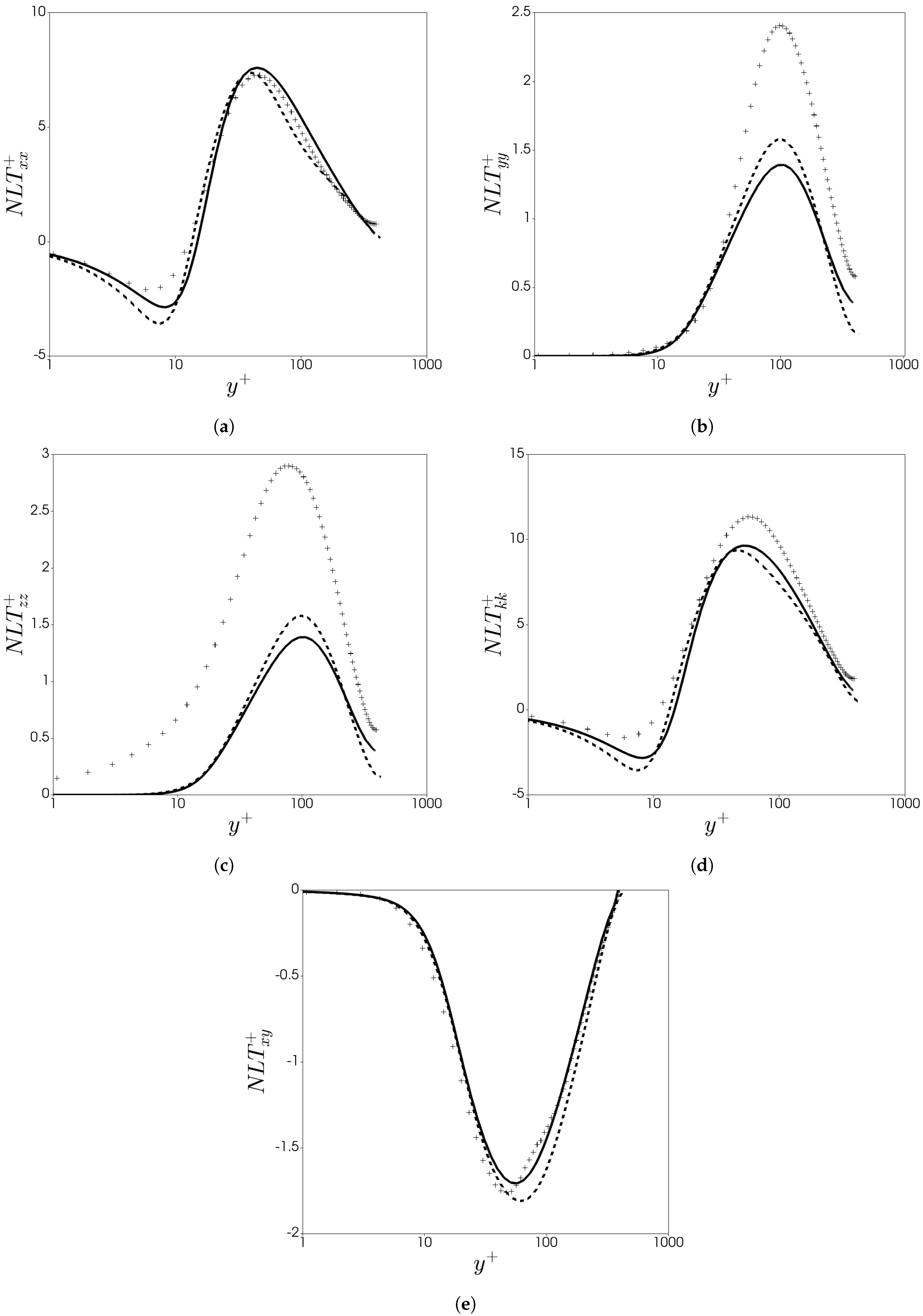
The performance of the N L T i j closure can be analysed in Figure 1 by comparing the predictions with DNS data case (19) in Table 1, and with the model of Resende et al. [32]. Figure 1a–c plots each normal component of N L T i j , with the predictions as accurate as the previous model [32]. The new N L T x x component is capable of predicting the maximum value and peak location of the destruction effect away from the wall along with the negative part near the wall, but requires a much simpler closure. The closure performance becomes more noticeable at higher Reynolds numbers, in which the polymer extension is largely overestimated previously. The N L T y y component is the leading order term in the C y y component away from the wall, which is the dominant contributor to an effective polymeric viscosity. This strongly influences the turbulent dynamics according to Thais et al. [40] and Benzi et al. [41] with their DNS and toy model analysis respectively. This term is represented by the first term in Equation (26), along with N L T z z . The N L T z z component was shown by Pinho et al. [20] to have low impact, and thus N L T z z = N L T y y is an appropriate approximation. The shear component, N L T x y , can be viewed in Figure 1e, where the predictions omit similar results compared with the previous model [32], but do not require additional L 2 variation via L 0.15 .
Overall, all main features of N L T i j are well captured such as the peak locations and magnitudes, but with a much simpler closure for the dominant contributor of polymer stretch, N L T x x . Further, the N L T x y and N L T y y terms responsible for the polymer shear stress contribution in the momentum balance are featured, which were previously represented ad-hoc with friction velocity dependence [26,28] or misrepresented [30].

3.2. Model for the Modified Damping Function, f ν

There have been many attempts to predict the eddy viscosity reduction as flow viscoelasticity increases for drag-reducing flows. In the case of low-Reynolds k ε models for FENE-P fluids, this was examined firstly by Pinho et al. [20] for the LDR regime; then later by Resende et al. [24] for the IDR regime. In both cases, there was a consistent reduction in the magnitude of k as DR increased, contrary to the DNS findings [23]. Similar attempts to model a modified damping function were made by Pinho [15]; Cruz et al. [16]; Resende et al. [17] and Tsukahara and Kawaguchi [31] to develop viscoelastic turbulence models using different constitutive equations.
Recently, Resende et al. [32] proposed a modified damping function which was able to predict the correct behavior of the eddy viscosity close to the wall, leading to the appropriate increase for the magnitude of k, and the shift away from the wall into the buffer layer as DR increased. This proposal was founded from the a-priori DNS data analysis by Resende et al. [42], demonstrating the necessary increase to the production of k close to the wall. The model derived by Resende et al. [32] is based on the DNS analysis of Li et al. [23], with an approximation of the form DR C k k / L , giving rise to the correct damping of near-wall eddies as DR increases. In the k ε v 2 f models proposed by Iaccarino et al. [26] and Masoudian et al. [28], the near-wall eddy viscosity damping effect is achieved by v 2 , as ν T = C μ v 2 k / ε . However, the reduction in v 2 is not enough to increase k as given by the DNS data.
The approach by Resende et al. [32] works well in increasing k in the buffer layer, but fails to capture the viscoelastic effects away from the wall, due to the fact that f μ Previous 1 as y h , which is contrary to the DNS data of Li et al. [22] and the analogous behavior of v 2 away from the wall. Therefore an additional model is required to capture the effect of nonequilibrium away from the wall, similarly to the Newtonian model of Park et al. [43]. Benzi et al. [41] demonstrated that the overall effect of polymer stretching is to introduce an effective viscosity proportional to C y y , which is dominated by the N L T y y component (modeled here with the first term in Equation (26)). An additional term is multiplied to the eddy viscosity to account for the global reduction of eddy structures for increasing DR. This approach is similar to the model of Resende et al. [24] and the study using DNS data of Resende et al. [42] which multiplies the damping function by a factor of 1 g ( VE ) , where g ( VE ) is a function of the viscoelastic terms, VE.
The final model presented for the modified damping function, f ν , is
f ν = 1 A 1 exp y * a μ 1 + B / a μ 2 ,
A = C A f N λ 2 L ˜ 3 / 2 f ( C k k ) 2 ε ν 0 0.3 ,
B = C B ( C k k 3 ) 1.25 / L ,
with model constants C A = 0.071 and C B = 0.44 . An additional contribution in the present model comes from an alternative representation of the dimensionless wall scaling y + = u τ / ν w , where ν w is the wall viscosity. The presence of the wall friction velocity poses a problem for flows with re-circulation or reattachment were the friction velocity becomes null at these points, causing floating point errors within computational solvers. Possibilities other than y + that solve this issue are R e y k y / ν 0 or the turbulent Reynolds number, R e t . Wallin and Johansson [44] formulated an alternative scaling, y * , in terms of R e y so that y * y + for y + 100 in channel flows. The form proposed is
y * = C y 1 R e y 1 / 2 + C y 2 R e y 2 ,
where C y 1 = 2.4 and C y 2 = 0.003 . The R e y -term is motivated by the fact that the near-wall asymptotic behaviour for R e y 1 / 2 is y 2 . The R e y 2 -term is artificially introduced to obtain a near linear relation in the buffer region.
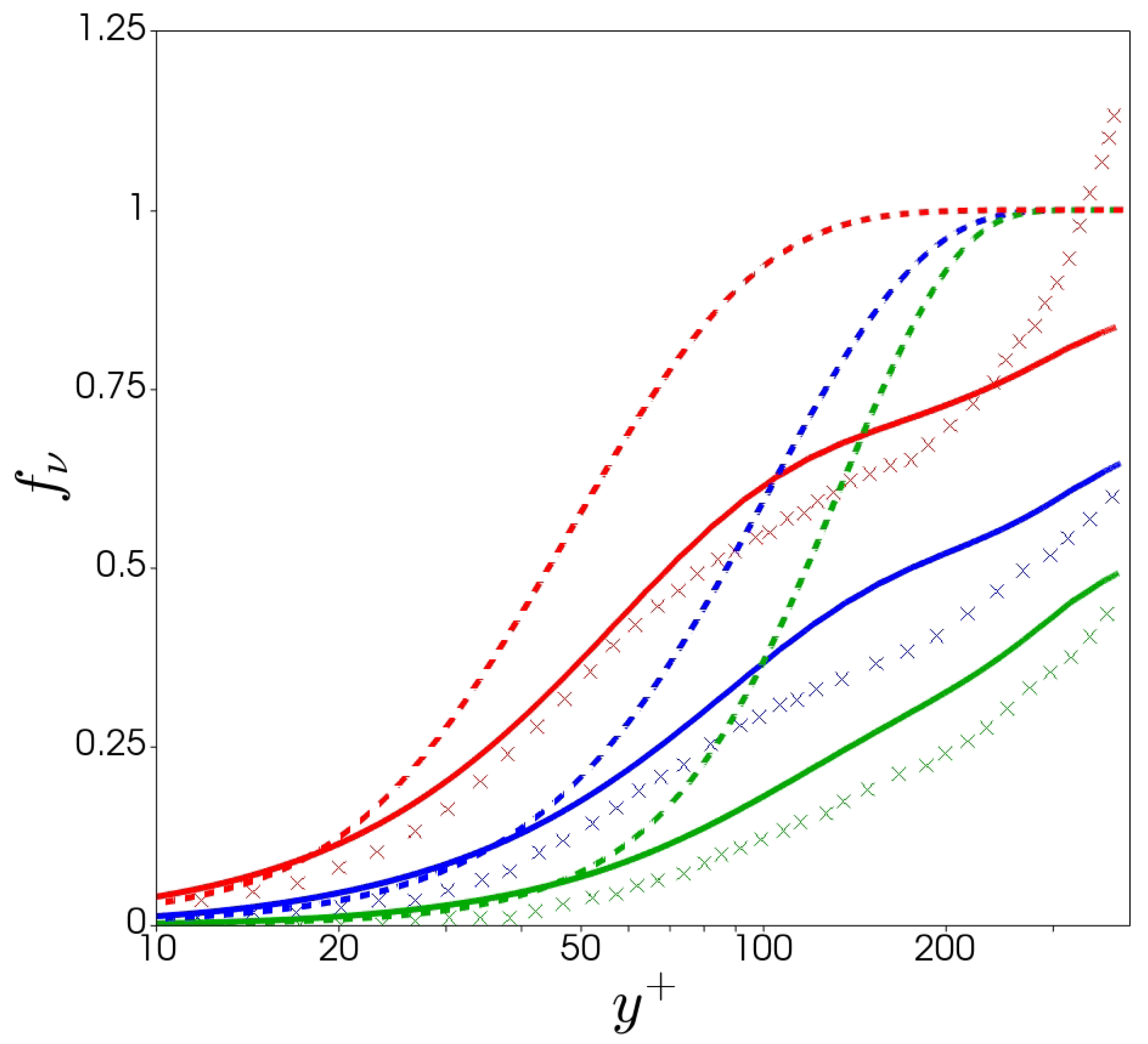
The performance of the f ν closure can be analyzed in Figure 2 by comparing the predictions with DNS data cases (16, 19, 20) for LDR, IDR and HDR respectively in Table 1 and with the model of Resende et al. [32]. The predictions offer significant improvement away from the wall compared to the previous model. The effects can be viewed for the turbulent kinetic energy and the eddy viscosity in the results section, offering improved results for various levels of DR and Reynolds numbers. The f ν closure more accurately represents the anisotropic effect akin to the v 2 f models of Masoudian et al. [28,30], with the thickening of the buffer layer from the stretched polymers, along with a global reduction with the new closure.

3.3. Development of Closures for ε V and E τ p

The closure model for ε V is approached following the DNS budget analysis of the governing terms proposed by Pinho et al. [20]. In their work, they verified that the double correlation can be neglected with respect to the triple correlation at LDR. This was later confirmed for IDR and HDR by Resende et al. [24] and Masoudian et al. [28], respectively. Pinho et al. [20] extended this analysis and demonstrated that the triple correlation can be decoupled and modeled as a function of N L T m m / 2 . Following this, Masoudian et al. [28] confirmed the model capabilities within 5% accuracy for all DR regimes via an extensive pdf study, and is the model used here given by
ε V ν p 2 λ f ( C m m ) N L T m m .
The closure model derived for E τ p assumes that it depends on the same quantities as the classical Newtonian destruction term of the transport equation of ε , but involving a viscoelastic quantity, typically with the viscoelastic stress work used by Resende et al. [24,32] and Masoudian et al. [28,30]. However, as ε V contains a negative part close to the wall via the N L T m m contribution, it is not feasible to include ε V in a suitable model for E τ P , based on the DNS analysis of ε being strictly decreasing near the wall for increasing DR.
The closure derived by Resende et al. [32] is complex with W i τ 0 dependence to force the correct trend in ε . Here, a much simpler approach is obtained with dependence through k and some viscoelastic quantities which increases proportional with DR. The closure is given by
E τ p C N 4 ε ˜ N k ν p C μ f μ L ˜ 3 / 4 k ν 0 2 ,
with model constant C N 4 = 0.083 . The effect of Equation (33) on ε predictions can be viewed in the results section for LDR and HDR.
Overall, it is clear that all the developed viscoelastic closures presented in this study perform well compared with DNS data. Most importantly, this was achieved without the use of friction velocity dependence. The simplicity of the governing closures allows easy implementation into 3D codes and can be extended to flows with reattachment when DNS data becomes available.

4. Summary of the Present Model

The governing equations with complete closure models that were developed in the previous sections are presented here.
Momentum equation:
ρ D U i D t = p ¯ x i + ρ x k ( ν s + ν T ) U i x k + ρ x k ν p λ f ( C n n ) C i k δ i k ,
where the eddy viscosity is given by
ν T = C μ f ν k 2 ε N ,
with modified damping function
f ν = 1 A 1 exp y * a μ 1 + B / a μ 2 ,
A = C A f N λ 2 L ˜ 3 / 2 f ( C k k ) 2 ε ν 0 0.3 ,
B = C B ( C k k 3 ) 1.25 / L ,
with constants a μ = 26.5 , C A = 0.071 and C B = 0.44 . y * is given by Equation (31).
Conformation tensor equation:
D C i j D t M i j N L T i j = 1 λ [ f ( C k k ) C i j δ i j ] ,
with
N L T i j f N C N 1 λ L ˜ ε N ν 0 f ( C m m ) δ i j f N 1 / 4 C N 2 M i j + C N 3 k ν 0 L ˜ M n n γ ˙ U i x k U j x k γ ˙ 2 ,
where f N = ν T / ν 0 is the local eddy viscosity, γ ˙ = 2 S p q S p q is the shear rate invariant, L ˜ = L 2 / 900 is the normalised maximum extension with the lowest DR, with model constants C N 1 = 0.11 , C N 2 = 0.3 and C N 3 = 0.3 .
Transport equation of k:
ρ D k D t = ρ x i ν s + f t ν T σ k k x i + P k ρ ( ε ˜ N + D ) ν p λ f ( C m m ) N L T m m 2 ,
where P k = ρ u i u j ¯ U i x j is the rate of production of k.
Dissipation transport equation:
ρ D ε ˜ N D t = ρ x i ν s + f t ν T σ ε ε ˜ N x i f 2 C ε 2 ρ ( ε ˜ N ) 2 k + ρ E + C ε 1 P k C N 4 ν p C μ f μ L ˜ 3 / 4 k ν 0 2 ε ˜ N k ,
with model constant C N 4 = 0.083 .
The remaining constants are from the Newtonian model and are C ε 1 = 1.45 , C ε 2 = 1.90 , C μ = 0.09 , σ k = 1.1 and σ ε = 1.3 .

5. Numerical Procedure

This section presents the numerical methods applied in order to examine the viscoelastic turbulence model against the available DNS data identified within the literature. A new finite volume C++ computational solver was developed in the OpenFOAM software by modifying the k ε sub-class files and introducing the FENE-P viscoelastic quantities such as: the polymer stress to the momentum equation; conformation tensor transport equation; and modified damping function to include elastic effects.
A fully-developed channel flow using half of the channel height, h, is applied given the symmetry of the governing geometry. We assigned 100 cells in the transverse (wall) direction with approximately 10 cells located inside the viscous sublayer. This is to provide mesh independent results, with errors within 0.5% for the mean velocity and the friction factor compared with a very fine mesh, similarly with [30]. The initial state of the simulation is the Newtonian solution until a steady-state solution was reached for each run case, except for HDR where a similar IDR developed case is applied to reduce computational time. Relaxation factors for the additional conformation tensor field are set to 0.2, along with residual control set to 10 5 . To improve numerical stability, an artificial diffusion term is added to the RACE of the form, κ k 2 C i j , where κ denotes a constant, isotropic, artificial numerical diffusivity. In earlier studies [10], the dimensionless artificial numerical diffusivity is taken to be κ / h u τ O ( 10 2 ) . Here, κ / h u τ O ( 10 3 ) and has negligible effect on mean values.
A pressure gradient is forced in the stream-wise direction to be unity, with periodic boundary conditions for all other flow fields, mimicking the DNS procedure of Li et al. [22]. No-slip boundary conditions were imposed on the solid wall for the velocity field U, along with k and ε ˜ set to zero (or very small, 10 15 ). A Dirichlet boundary condition for C i j is reported in Appendix A (similar to [26], but for all components), which is imposed within OpenFOAM under the swak4Foam library using the groovyBC functionality developed by Gschaider [45].
When normalizing the governing equations and inherently the various physical quantities, the velocity scale is taken to be the friction velocity (leading to the use of superscript +) and the length scale is the viscous length, x i = x i + ν 0 / U τ . The conformation tensor is already in dimensionless form.

6. Results and Discussion

Following the numerical procedure proposed in the previous section, the model performance is assessed against a range of different flow and rheological parameters presented in the DNS data within Table 1.

6.1. Analysis of Conformation Tensor

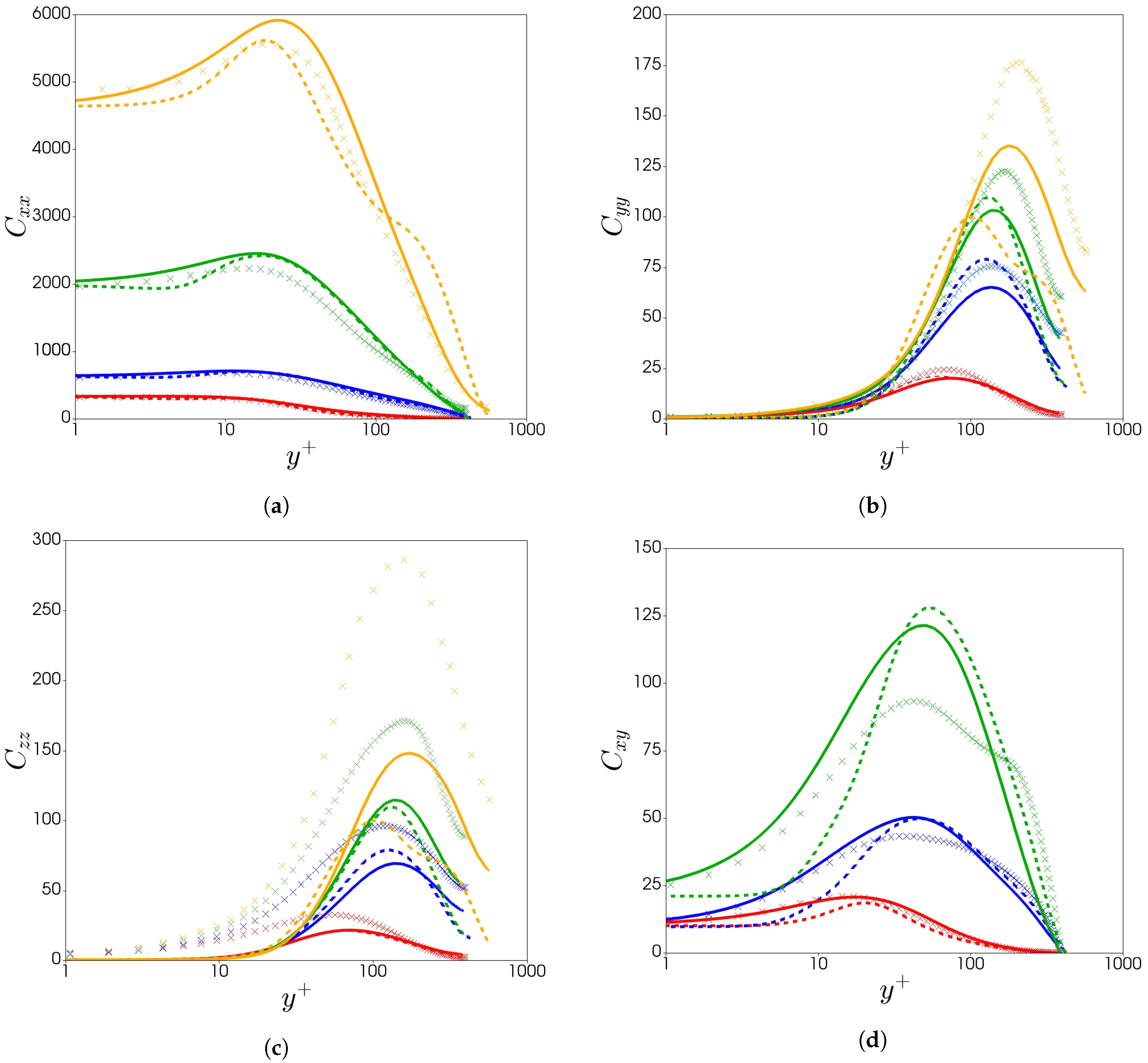
Figure 3 compares the individual components of the conformation tensor with the present model against the model of Resende et al. [32] and selected DNS data covering L 2 , W i τ 0 and R e τ 0 variations (cases 16, 19, 20 and 26 in Table 1). as can be viewed in Figure 3a, the C x x predictions are consistent with the DNS data. The new closure for N L T x x (see term III in Equation (26)) is responsible for the improved predictions and can capture the R e τ 0 , L 2 and W i τ 0 variations with much greater simplicity, especially for increased Reynolds number ( R e τ 0 = 590 ) compared with the model of Resende et al. [32].
Figure 3b plots the C y y component, showing good agreement with the DNS data and improving upon the most recent model, especially away from the wall. The important feature is the location of the value at the centre-line and the peak location which both show good improvement, especially for higher Reynolds numbers ( R e τ 0 = 590 ). The improvements are a result of the new E τ p closure (see Equation (33)) which directly impacts ε N in the N L T y y closure (see term I in Equation (26)). Figure 3c plots the C z z component and shows an under-prediction due to the isotropic assumption used in the model of N L T i j , however, its impact is not significant.
The model predictions of the C y y term are important in capturing the features of the C x y component. As can be observed in Figure 3d, the model is able to capture the near-wall region, which, according to the findings of Li et al. [22], is the region of high chain dumbbell extension (limited to y + < 50 ) where the effect of C x y acts towards the polymer shear stress.
It is evident that the overall predictions of the individual conformation tensor components are improved compared to the model of Resende et al. [32]. This is a result of the new N L T i j and E τ p closures developed in the present work, which allows more scope of predictability and increased numerical stability with simpler closures.

6.2. Analysis of k, ε and ν T

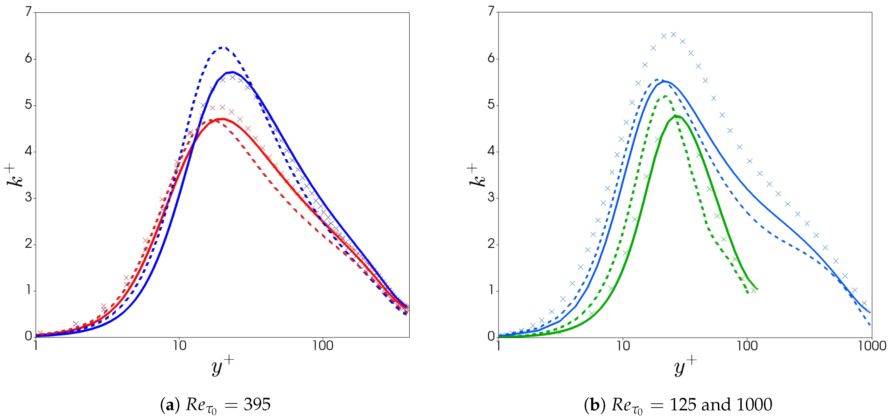
The predicted k profiles are shown in Figure 4a for cases 16 and 19 in Table 1, and Figure 4b for low and high Reynolds number cases (7 and 27). There is reasonable improvement of the profile away from the wall as a result of the new f ν closure for increasing drag reduction and for various Reynolds numbers.
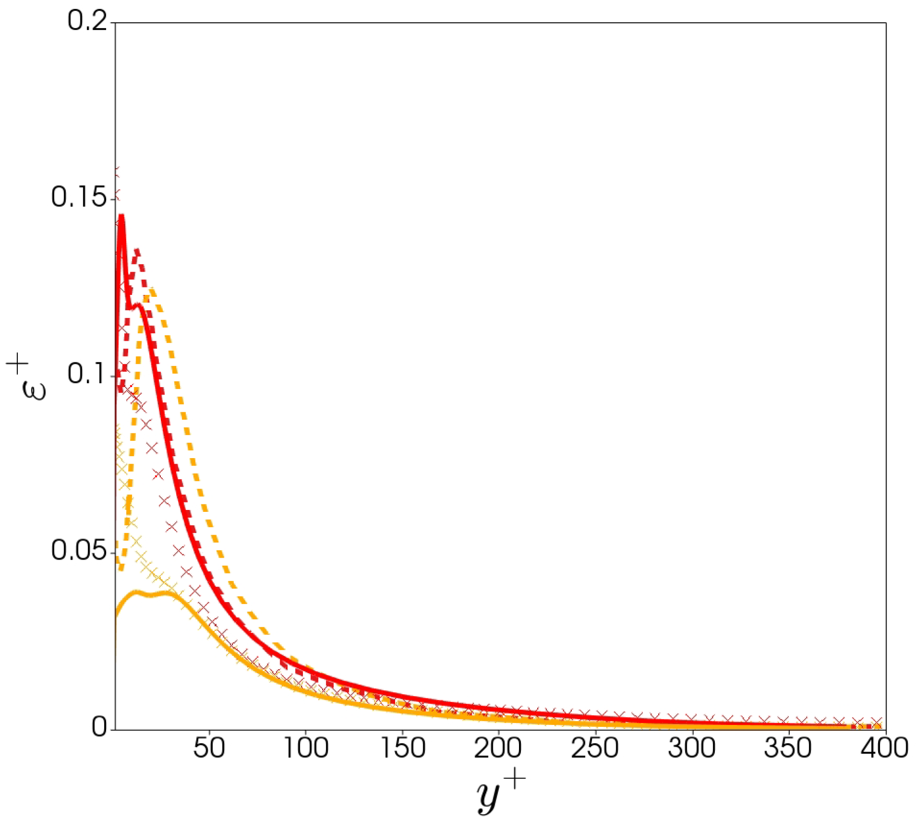
In Figure 5, the prediction of the dissipation rate are compared with the DNS data of both LDR (case 16) and very HDR (case 22), along with predictions for the v 2 f model of Masoudian et al. [28]. The predictions for LDR are captured well with the DNS for both near and far from the wall. For HDR, there is a significant improvement near the wall compared with the v 2 f model. This is a result of the E τ p closure formulated (See Equation (33)) which decreases ε as flow viscoelasticity increases. The model of Resende et al. [32] shows similar results to the current model and is not plotted so that the figure is clearer. However, the complexity of the present E τ p closure model is reduced substantially and removes all friction velocity dependence, but can still predict all the main flow features with good performance.
The local eddy viscosity is plotted in Figure 6a for all ranges of DR. The combined performance of f ν , k and ε gives rise to the predictions shown. We observe a reduction in the eddy structures within the buffer-layer and log-layer for increasing DR, as the DNS suggests. The damping function predicts well this behavior with the near-wall polymer extension via C k k and the global reduction via ( 1 A ) .

6.3. Analysis of Velocity Profiles

Figure 6b shows the mean stream-wise velocity profiles for all ranges of DR at R e τ 0 = 395 . All of the profiles reduce to the linear distribution u + = y + in the viscous sub-layer. Further from the wall, the velocity profiles are well-captured for all ranges of DR.
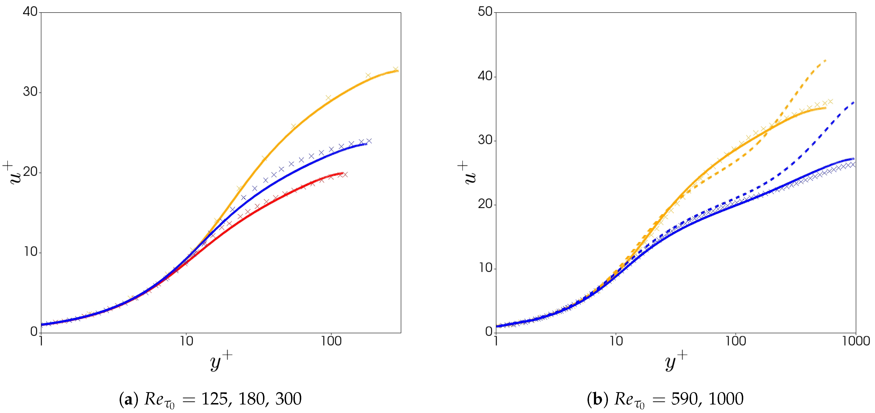
The model can also predict well a range of Reynolds numbers with varying rheological parameters as can be viewed in Figure 7a. This is extended in Figure 7b for high Reynolds numbers, where there is a significant improvement compared with the model of Resende et al. [32]. This is a result of the new closure model for N L T x x which scales well with Reynolds number and with reduced complexity.
The advantage of the current model is the ability to capture all velocity profiles well within the model limits, with more simplicity with regards to model closures and without friction velocity dependence.

7. Conclusions

A viscoelastic turbulence model in fully-developed drag-reducing channel flow is improved, with turbulent eddies modeled under a k ε representation, along with polymeric solutions described by the finitely extensible nonlinear elastic-Peterlin (FENE-P) constitutive model. A new finite volume C++ computational solver was developed in the OpenFOAM software by modifying the k ε sub-class files and introducing the FENE-P viscoelastic quantities such as: the polymer stress to the momentum equation; conformation tensor transport equation; and modified damping function to include elastic effects. The model performance is evaluated against a variety of rheological parameters within the DNS data literature, including: friction Reynolds number R e τ 0 = 125 , 180 , 300 , 395 , 590 , 1000 ; Wiessenberg number W i τ 0 = 25 , 36 , 50 , 100 , 116 , 200 ; and maximum molecular extensibility of the dumbbell chain L 2 = 900 , 1800 , 3600 , 10,000 , 14,400 . The DNS data case (19) in Table 1 ( R e τ 0 = 395 , DR = 37%) is used for the calibration of the closures developed for the turbulent cross-correlations identified in Section 3. The model is capable of predicting all flow features for low and high Reynolds numbers at all regimes of DR and improves significantly on the model of Resende et al. [32], with its ability to capture higher Reynolds numbers with simpler and physical-based closures.
The main feature is the formulation of the N L T i j term which accounts for the interactions between the fluctuating components of the conformation tensor and the velocity gradient tensor. The advantage of the closure is the reduction in the complexity and use of damping functions in the dominant contribution, N L T x x , modeled here to increase with turbulent kinetic energy as the flow viscoelasticity increases, demonstrating significant improvement with a range of rheological parameters and flow conditions.
Further improvements are developed for the viscoelastic destruction term, E τ p , within the dissipation rate transport equation. Modeled here with dependence on k and viscoelastic quantities, showing the ability to predict ε for low and high drag reduction.
An improved modified damping function, f ν , is also presented, which is able to predict the global reduction of the eddy viscosity and shift away from the wall for increasing viscoelasticity, whilst also improving the profiles of turbulent kinetic energy.
Overall, predictions compare very well with a wide range of DNS data and significantly improves on capturing all flow features with simplicity and performance compared with the most recent k ε model developed by Resende et al. [32]. The simplicity of the present model allows easy implementation into 3D codes and increases numerical stability. All friction velocity dependence is removed in the present model which is the first of its kind for damping function k ε models, whose main advantage is the realization of simulations in geometries with reattachment. Future work to extend to this study includes the development of an improved k ω model based on the present model [25]. This would require the same concept of the modified damping function developed in this paper to be applied, with capabilities to predict flow behavior in industrially represented geometries such as pipes and constrictions.
Author Contributions

Supervision: P.R., T.C., M.W., A.A., D.H. and G.d.B.; software: M.M., G.d.B. and A.A.; formal analysis: M.M., P.R., M.W. and G.d.B.; project administration: T.C., M.W., D.H. and G.d.B. All authors have read and agreed to the published version of the manuscript.

Funding

This research was funded by Engineering and Physical Sciences Research Council (EPSRC) [Grant number: EP/N5059681/1, Award Reference: 1958044].

Conflicts of Interest

The authors declare no conflict of interest.

Appendix A

The FENE-P equations simplify considerably if we consider 1D, laminar, parallel flow: u x = u z = 0 and u x = u x ( y ) u . The system becomes:
C y y d u d y 1 λ ( f ( C k k ) C x y ) = 0
1 λ 1 f ( C k k ) C y y = 0
1 λ 1 f ( C k k ) C z z = 0
2 C x y d u d y 1 λ 1 f ( C k k ) C x x = 0 ,
where f ( C k k ) = L 2 L 2 C k k . Introducing the Weissenberg number as W i = λ d u d y and solving the system of equations above, one finds the following cubic equation in f ( C k k ) f :
f 3 f 2 2 W i 2 L 2 = 0 ,
which omits one real solution, f R , that satisfies the laminar equations applicable at the wall:
C x x = 1 f R 2 W i 2 f R 2 + 1
C y y = 1 f R
C z z = 1 f R
C x y = W i f R 2
where
f R = 1 3 B 2 1 / 3 + 2 1 / 3 B + 1
with
B = ( A + [ ( A + 2 ) 2 4 ] 1 / 2 + 2 ) 1 / 3 and A = 54 W i L 2 .
In our numerical simulations, the explicit definition of the wall value using Equations (A6)–(A9) as a Dirichlet boundary condition considerably improves the stability of the solution procedure and is preferred over a zero-flux Neumann boundary condition for the conformation tensor.

References

  1. Toms, B.A. Some observations on the flow of linear polymer solutions through straight tubes at large Reynolds numbers. Proc. Int. Cong. Rheol. 1948, 2, 135–141. [Google Scholar]
  2. Virk, P.S. Drag reduction fundamentals. AIChE J. 1975, 21, 625–656. [Google Scholar] [CrossRef]
  3. Lumley, J.L. Drag reduction by additives. Annu. Rev. Fluid Mech. 1969, 1, 367–384. [Google Scholar] [CrossRef]
  4. Lumley, J.L. Drag reduction in turbulent flow by polymer additives. J. Polym. Sci. Macromol. Rev. 1973, 7, 263–290. [Google Scholar] [CrossRef]
  5. Hoyt, J. A Freeman scholar lecture: The effect of additives on fluid friction. J. Fluids Eng. 1972, 94, 258–285. [Google Scholar] [CrossRef]
  6. Virk, P.S.; Merrill, E.; Mickley, H.; Smith, K.; Mollo-Christensen, E. The Toms phenomenon: Turbulent pipe flow of dilute polymer solutions. J. Fluid Mech. 1967, 30, 305–328. [Google Scholar] [CrossRef] [Green Version]
  7. White, C.M.; Mungal, M.G. Mechanics and prediction of turbulent drag reduction with polymer additives. Annu. Rev. Fluid Mech. 2008, 40, 235–256. [Google Scholar] [CrossRef]
  8. Procaccia, I.; L’vov, V.S.; Benzi, R. Colloquium: Theory of drag reduction by polymers in wall-bounded turbulence. Rev. Mod. Phys. 2008, 80, 225. [Google Scholar] [CrossRef] [Green Version]
  9. Dubief, Y.; Terrapon, V.E.; White, C.M.; Shaqfeh, E.S.; Moin, P.; Lele, S.K. New answers on the interaction between polymers and vortices in turbulent flows. Flow Turbul. Combust. 2005, 74, 311–329. [Google Scholar] [CrossRef]
  10. Sureshkumar, R.; Beris, A.N.; Handler, R.A. Direct numerical simulation of the turbulent channel flow of a polymer solution. Phys. Fluids 1997, 9, 743–755. [Google Scholar] [CrossRef]
  11. L’vov, V.S.; Pomyalov, A.; Procaccia, I.; Tiberkevich, V. Drag reduction by polymers in wall bounded turbulence. Phys. Rev. Lett. 2004, 92, 244503. [Google Scholar] [CrossRef] [Green Version]
  12. De Angelis, E.; Casciola, C.M.; L’vov, V.S.; Pomyalov, A.; Procaccia, I.; Tiberkevich, V. Drag reduction by a linear viscosity profile. Phys. Rev. E 2004, 70, 055301. [Google Scholar] [CrossRef] [Green Version]
  13. Dallas, V.; Vassilicos, J.C.; Hewitt, G.F. Strong polymer-turbulence interactions in viscoelastic turbulent channel flow. Phys. Rev. E 2010, 82, 066303. [Google Scholar] [CrossRef] [Green Version]
  14. Min, T.; Yoo, J.Y.; Choi, H.; Joseph, D.D. Drag reduction by polymer additives in a turbulent channel flow. J. Fluid Mech. 2003, 486, 213–238. [Google Scholar] [CrossRef] [Green Version]
  15. Pinho, F. A GNF framework for turbulent flow models of drag reducing fluids and proposal for a kε type closure. J. Non-Newton. Fluid Mech. 2003, 114, 149–184. [Google Scholar] [CrossRef]
  16. Cruz, D.; Pinho, F.; Resende, P. Modelling the new stress for improved drag reduction predictions of viscoelastic pipe flow. J. Non-Newton. Fluid Mech. 2004, 121, 127–141. [Google Scholar] [CrossRef]
  17. Resende, P.; Escudier, M.; Presti, F.; Pinho, F.; Cruz, D. Numerical predictions and measurements of Reynolds normal stresses in turbulent pipe flow of polymers. Int. J. Heat Fluid Flow 2006, 27, 204–219. [Google Scholar] [CrossRef]
  18. Resende, P.; Pinho, F.; Cruz, D. A Reynolds stress model for turbulent flows of viscoelastic fluids. J. Turbul. 2013, 14, 1–36. [Google Scholar] [CrossRef]
  19. Leighton, R.; Walker, D.T.; Stephens, T.; Garwood, G. Reynolds stress modeling for drag reducing viscoelastic flows. In Proceedings of the ASME/JSME 2003 4th Joint Fluids Summer Engineering Conference, Honolulu, HI, USA, 6–10 July 2003; American Society of Mechanical Engineers: New York, NY, USA, 2003; pp. 735–744. [Google Scholar]
  20. Pinho, F.; Li, C.; Younis, B.; Sureshkumar, R. A low Reynolds number turbulence closure for viscoelastic fluids. J. Non-Newton. Fluid Mech. 2008, 154, 89–108. [Google Scholar] [CrossRef]
  21. Housiadas, K.D.; Beris, A.N.; Handler, R.A. Viscoelastic effects on higher order statistics and on coherent structures in turbulent channel flow. Phys. Fluids 2005, 17, 035106. [Google Scholar] [CrossRef]
  22. Li, C.; Gupta, V.; Sureshkumar, R.; Khomami, B. Turbulent channel flow of dilute polymeric solutions: Drag reduction scaling and an eddy viscosity model. J. Non-Newton. Fluid Mech. 2006, 139, 177–189. [Google Scholar] [CrossRef]
  23. Li, C.F.; Sureshkumar, R.; Khomami, B. Influence of rheological parameters on polymer induced turbulent drag reduction. J. Non-Newton. Fluid Mech. 2006, 140, 23–40. [Google Scholar] [CrossRef]
  24. Resende, P.; Kim, K.; Younis, B.; Sureshkumar, R.; Pinho, F. A FENE-P kε turbulence model for low and intermediate regimes of polymer-induced drag reduction. J. Non-Newton. Fluid Mech. 2011, 166, 639–660. [Google Scholar] [CrossRef]
  25. Resende, P.; Pinho, F.; Younis, B.; Kim, K.; Sureshkumar, R. Development of a Low-Reynolds-number k-ω Model for FENE-P Fluids. Flow Turbul. Combust. 2013, 90, 69–94. [Google Scholar] [CrossRef]
  26. Iaccarino, G.; Shaqfeh, E.S.; Dubief, Y. Reynolds-averaged modeling of polymer drag reduction in turbulent flows. J. Non-Newton. Fluid Mech. 2010, 165, 376–384. [Google Scholar] [CrossRef]
  27. Dubief, Y.; Laccarino, G.; Lele, S. A Turbulence Model for Polymer Flows; Center for Turbulence Research: Stanford, CA, USA, 2004. [Google Scholar]
  28. Masoudian, M.; Kim, K.; Pinho, F.; Sureshkumar, R. A viscoelastic kε–v2–f turbulent flow model valid up to the maximum drag reduction limit. J. Non-Newton. Fluid Mech. 2013, 202, 99–111. [Google Scholar] [CrossRef]
  29. Masoudian, M.; Kim, K.; Pinho, F.; Sureshkumar, R. A Reynolds stress model for turbulent flow of homogeneous polymer solutions. Int. J. Heat Fluid Flow 2015, 54, 220–235. [Google Scholar] [CrossRef]
  30. Masoudian, M.; Pinho, F.; Kim, K.; Sureshkumar, R. A RANS model for heat transfer reduction in viscoelastic turbulent flow. Int. J. Heat Mass Transf. 2016, 100, 332–346. [Google Scholar] [CrossRef]
  31. Tsukahara, T.; Kawaguchi, Y. Proposal of damping function for low-Reynolds-number-model applicable in prediction of turbulent viscoelastic-fluid flow. J. Appl. Math. 2013, 2013. [Google Scholar] [CrossRef] [Green Version]
  32. Resende, P.; Afonso, A.; Cruz, D. An improved k-ε turbulence model for FENE-P fluids capable to reach high drag reduction regime. Int. J. Heat Fluid Flow 2018, 73, 30–41. [Google Scholar] [CrossRef] [Green Version]
  33. Bird, R.B.; Armstrong, R.C.; Hassager, O. Dynamics of Polymeric Liquids, Volume 1: Fluid Mechanics; Wiley: New York, NY, USA, 1987. [Google Scholar]
  34. Alfonsi, G. Reynolds-averaged Navier–Stokes equations for turbulence modeling. Appl. Mech. Rev. 2009, 62, 040802. [Google Scholar] [CrossRef]
  35. Nagano, Y.; Hishida, M. Improved form of the k-ε model for wall turbulent shear flows. J. Fluids Eng. 1987, 109, 156–160. [Google Scholar] [CrossRef]
  36. Nagano, Y. Modeling the dissipation-rate equation for two-equation turbulence model. In Proceedings of the 9th Symposium on Turbulent Shear Flows, Kyoto, Japan, 16–18 August 1993; p. 23. [Google Scholar]
  37. Thais, L.; Gatski, T.B.; Mompean, G. Some dynamical features of the turbulent flow of a viscoelastic fluid for reduced drag. J. Turbul. 2012, 13, N19. [Google Scholar] [CrossRef]
  38. Thais, L.; Gatski, T.B.; Mompean, G. Analysis of polymer drag reduction mechanisms from energy budgets. Int. J. Heat Fluid Flow 2013, 43, 52–61. [Google Scholar] [CrossRef]
  39. Masoudian, M.; da Silva, C.; Pinho, F. Grid and subgrid-scale interactions in viscoelastic turbulent flow and implications for modelling. J. Turbul. 2016, 17, 543–571. [Google Scholar] [CrossRef]
  40. Thais, L.; Tejada-Martinez, A.; Gatski, T.; Mompean, G. Temporal large eddy simulations of turbulent viscoelastic drag reduction flows. Phys. Fluids 2010, 22, 013103. [Google Scholar] [CrossRef]
  41. Benzi, R. A short review on drag reduction by polymers in wall bounded turbulence. Phys. D Nonlinear Phenom. 2010, 239, 1338–1345. [Google Scholar] [CrossRef]
  42. Resende, P.; Cavadas, A. New developments in isotropic turbulent models for FENE-P fluids. Fluid Dyn. Res. 2018, 50, 025508. [Google Scholar] [CrossRef] [Green Version]
  43. Park, T.S.; Sung, H.J. A nonlinear low-Reynolds-number κ-ε model for turbulent separated and reattaching flows—I. Flow field computations. Int. J. Heat Mass Transf. 1995, 38, 2657–2666. [Google Scholar] [CrossRef]
  44. Wallin, S.; Johansson, A.V. An explicit algebraic Reynolds stress model for incompressible and compressible turbulent flows. J. Fluid Mech. 2000, 403, 89–132. [Google Scholar] [CrossRef]
  45. Gschaider, B.F. The incomplete swak4Foam reference. Tech. Rep. 2013, 131, 202. [Google Scholar]
Figure 1. Comparison of the N L T i j model between DNS data (+DR = 37%, case (19)) and predictions with the new model (continuum lines), and previous model (dash lines): (a) N L T x x + ; (b) N L T y y + ; (c) N L T z z + ; (d) N L T k k + ; (e) N L T x y + .
Applsci 10 08140 g001
Figure 2. Comparison of the f ν model between DNS data (× crosses) and predictions with the new model (continuum lines), and previous model (dash lines): each colour represents a different drag reduction regime: red (low drag reduction (LDR), case 16); blue (intermediate drag reduction (IDR), case 19); green (high drag reduction (HDR), case 20).
Applsci 10 08140 g002
Figure 3. Comparison of the conformation tensor between DNS data (× crosses) and predictions with the new model (continuum lines), and previous model (dash lines): (a) C x x ; (b) C y y ; (c) C z z ; (d) C x y . Each colour represents a different drag reduction regime: red (LDR, case 16); blue (IDR, case 19); green (HDR, case 20) and orange (very HDR, case 26. DNS data not available for C x y ).
Applsci 10 08140 g003
Figure 4. Comparison of turbulent kinetic energy between DNS data (× crosses) and predictions with the new model (continuum lines), and previous model (dash lines): (a) R e τ 0 = 395 —red (LDR case 16)—and blue (IDR case 19); (b) R e τ 0 = 125 —green (HDR, case 7) and R e τ 0 = 1000 —blue (IDR, case 27).
Applsci 10 08140 g004
Figure 5. Comparison of the rate of Newtonian dissipation of k between DNS data (× crosses) and predictions with the new model (continuum lines), and v 2 f model of Masoudian et al. [28] (dash lines). Each colour represents a different drag reduction regime: red (LDR case 16); orange (HDR case 22).
Applsci 10 08140 g005
Figure 6. Comparison of the (a) local eddy viscosity and (b) mean stream-wise velocity profile, between DNS data (× crosses) and model predictions (continuum lines). Each colour represents a different drag reduction regime: red (LDR case 16); blue (IDR case 19); green (HDR case 20); orange (very HDR case 22).
Applsci 10 08140 g006
Figure 7. Comparison of the velocity profiles between DNS data (× crosses), current model predictions (continuum lines) and previous model predictions [32] (dashed lines). Each colour represents a different drag reduction regime: (a) red (LDR case 1); blue (IDR case 10); orange (very HDR case 15). (b) blue (IDR case 27); orange (very HDR case 26).
Applsci 10 08140 g007
Table 1. Independent Direct Numerical Simulation data for turbulent channel flow of finitely extensible nonlinear elastic-Peterlin (FENE-P) fluids at β = 0.9 , with drag reduction (DR) model predictions.
CaseReferenceRheological ParametersDrag Reduction (%)
Re τ 0 Wi τ 0 L 2 DNSCurrent ModelModel [32]
(1)Li et al. [23]125259001920-
(2)Li et al. [23]1252536002223-
(3)Li et al. [23]1252514,4002425-
(4)Li et al. [23]12550900313035
(5)Li et al. [23]125100900373639
(6)Li et al. [23]12510018004543-
(7)Li et al. [23]1251003600565151
(8)Masoudian et al. [28]180259001919-
(9)Li et al. [23]18050900313034
(10)Masoudian et al. [28]180100900383839
(11)Masoudian et al. [28]1801003600545351
(12)Thais et al. [37]18011610,0006460-
(13)Iaccarino et al. [26]300363600333234
(14)Iaccarino et al. [26]3003610,000353532
(15)Iaccarino et al. [26]30012010,000595958
(16)Masoudian et al. [30]39525900192219
(17)Masoudian et al. [30]395509003030-
(18)Masoudian et al. [30]3955036003838-
(19)Masoudian et al. [30]395100900373738
(20)Masoudian et al. [30]3951003600484752
(21)Masoudian et al. [39]39510010,0005555-
(22)Masoudian et al. [30]39510014,400616062
(23)Thais et al. [37]39511610,0006260-
(24)Li et al. [23]39520014,400756967
(25)Masoudian et al. [30]590503600394064
(26)Thais et al. [37]59011610,000615974
(27)Thais et al. [38]100050900303360
Publisher’s Note: MDPI stays neutral with regard to jurisdictional claims in published maps and institutional affiliations.