An Investigation of Radial Basis Function Method for Strain Reconstruction by Energy-Resolved Neutron Imaging

Abstract

The main objective of the current work is to determine meshless methods using the radial basis function (rbf) approach to estimate the elastic strain field from energy-resolved neutron imaging. To this end, we first discretize the longitudinal ray transformation with rbf methods to give us an unconstrained optimization problem. This discretization is then transformed into a constrained optimization problem by adding equilibrium conditions to ensure uniqueness. The efficiency and accuracy of this approach are investigated for the situation of 2d plane stress. In addition, comparisons are made between the results obtained with rbf collocation, finite-element (fem) and analytical solution methods for test problems. The method is then applied to experimentally measured continuous and discontinuous strain fields using steel samples for an offset ring-and-plug and crushed ring, respectively.

1. Introduction

Consider a solid material sample composed of similar crystals with a uniform distribution of directions. There are three times as many crystallographic planes in each crystal as there are Miller indices. The sample if subject to a narrow neutron beam with a known distribution of kinetic energy. The neutrons behave as waves with the energy inversely proportional to the wavelength, and this wavelength is a similar magnitude to the crystallographic planes [1,2]. Parallel crystallographic planes with d separation scatter an incident wave if the wavelength is a multiple of $2dsin\theta$. If we detect only the transmitted neutrons, the scattered neutrons will be lost. If we look the number of transmitted neutrons as a function of wavelength, then at the wavelength $2d$ the transmission leaps dramatically. This jump is labelled as the Bragg edges. If the material is subjected to a $\epsilon$ linear elastic strain, the separation between planes with a normal $\mathbf{n}$ vector is in proportion to the strain component $\mathbf{n}·\epsilon ·\mathbf{n}$. For more information and additional sources, see [3,4,5]. If the strain were consistent along the neutron path, the Bragg edge would be shifted. Within ideal conditions, a linear wavelength function multiplied by the unit step function can model the Bragg edges. Abbey et al. [6] had previously explored whether strain could be reconstructed from the average of each ray shifts of a Bragg edge. Lionheart and Withers [7] noted that the transverse ray transformation is feasible for X-ray strain measurements.

Given the longitudinal ray transformation (lrt) data plane by plane, an attempt could be made to recover the strain from the ray measurements in that plane using appropriate additional a priori information [8]. The Lamé system could be represented by finite-element or finite difference methods provided that the Lamé coefficients are known. A linear system could be developed, and the least square solution determined together with a discretization of the lrt and prior knowledge. This method has been adopted by Gregg et al. [5] for axisymmetric objects, Wensrich et al. [9] for synthetic data, and Henriks et al. [10] for a generic case experimentally.

We consider here the measurement of the Bragg edges based on the calculation of the propagation spectrum using flight time or energy-resolved technologies. We note that other approaches exist [3,11,12,13]. The major contribution of neutron transmission strain tomography is the optimal use of the incident beam flux to reduce the data collection time. Recent developments in detector technology allow the acquisition of high-resolution strain images with Bragg neutron transmission [14]. The sample is placed on a rotating plate between the source and a micro-channel plate detector (mcp) [15,16]. This detector is pixelated with a spatial resolution of up to $512\times 512$ pixels of up to 55 $\mathsf{\mu }$m. This imaging raises the possibility of strain tomography, and efforts have been made over the past few years to solve the resulting tensor reconstruction challenge—special cases such as axial symmetry revolved around reconstruction techniques [5,17]. A well-known fact about this inverse problems is that it is not well-posed. Therefore it is not possible to reconstruct the strain without the inclusion of additional conditions or without easing assumptions [10]. The question of how to better execute these additional criteria was discussed and various approaches were used in the literature [5,9]. Recently, reconstruction has been accomplished by incorporating either equilibrium or compatibility conditions. The main distinction between these approaches is the set of basis functions representing the strain field [6,10].

Recently, considerable attention has been given in the science and engineering community to the concept of using meshfree methods as a modern tool for numerical solution for partial differential equations. As stated in [18,19], the growing interest in these methods is due partly to their high versatility, particularly in the case of high-dimensional problems. Conventional grid-based approaches such as finite difference (FDM) [20] and finite-element (fem) [21] methods have inherent problems, namely a mesh generation requirement. Mesh generation is not a simple job, particularly for domains with irregular and complex geometries requiring additional mathematical transformations that can be as costly as solving the problem. Meshfree avoid this problem since the conventional definition of the concept does not include the meshing procedure. This makes it easy to understand the behavior of complex solids, structures and stress and strain fields arbitrarily distributed in the domain without any constraints. Moreover, we do not need to consider the connectivity between the nodes while applying the meshfree process. For a survey of various meshless approaches and underlying findings, we refer the reader to [22,23,24,25].

The paper describes a meshless process by which the elastic strain of a series of Bragg-edge strain measurements can be reconstructed tomographically. Because of the attractive properties of radial basis functions (rbf), the approach has some advantages over previous approaches. Especially its ability to represent extremely spatially varying functions accurately. The proposed algorithm is evaluated on a two-dimensional simulated beam data for which a thorough comparison of the fem and rbf methods is shown. It is shown to be able to reconstruct a tensor field, after [26,27] imposed equilibrium conditions. The framework is then extended to real experiment measurements for the steel geometry of an offset ring-and-plug and a crushed ring.

The paper has the following structure: Section 2 discusses strain measurement through the Longitudinal Ray Transformation. Section 3 offers an overview and algorithm of the meshless method for strain field reconstruction and presents the proposed algorithm structure and the finite-element approach. Section 4 addresses the validation of the algorithm using a cantilevered beam and the key difference between the fem and the solution being suggested. Finally, the experimental findings with the ring-and-plug and crushed ring steel samples are addressed in Section 5. Section 6 summarizes the work in this paper and lists the work to be done in the future.

2. Strain Measurement

Here we discuss the recent experimental method that provides information on the average strain component for the set of incident neutron beam [11]. This approach can have a significant influence in several experimental fields in mechanics. Bragg-edge strain tomography guarantees a unique structured approach for the study of materials with residual stress field over practical scales. The Bragg edges, as mentioned above, are generated by backscattering radiation. As a result, relative shifts in their position calculate the average normal strain of the sample towards the ray [28]. This challenge revolves around the lrt inversion, which represents an effective measurement process model. Although this is a three-dimensional problem in general, for convenience, this article takes only two dimensions into account. The average strain within the body measured by Bragg-edge neutron transmission is often idealized as a longitudinal line integral, namely lrt, which captures the average strain component along the line towards the normal unit direction $\mathbf{n}={(n_1,n_2)}^T$. ${\mathsf{\Gamma }}_{\epsilon }$ is a form of ray transform specifically known as lrt. Hence, lrt shown in Figure 1 with reference to the coordinate system and geometry is defined as

$${\mathsf{\Gamma }}_{\epsilon }(x,y,\vartheta )=\frac{1}{L}\left[\sum _{i=1}^2\sum _{j=1}^2{\int }_0^L{n}_i{\epsilon }_{ij}(x(s,a),y(s,a))n_{j}ds\right],$$

(1)

where ${\epsilon }_{ij}$ is the $(i,j)th$ component of tensor strain field $\epsilon \in {\mathbf{R}}^{2\times 2}$, which is mapped to an average normal component of a strain in the direction of $\widehat{\mathbf{n}}$. A ray projection enters the sample at the location ${\mathbf{x}}_a=(x(s,a),y(s,a))$, where s is the ray propagation distance coordinate and L is the length of the ray within the sample at the particular angle. Every pixel of a strain image measures the average normal strain in the ray direction through the thickness of the domain, say ${\mathsf{\Gamma }}_{\epsilon }$. It is based on the overall change of the gauge distance within that ray [6,7]. Measurements are taken in each orientation, ${\vartheta }_i$, where the profile is calculated in the form ${\mathsf{\Gamma }}_{\epsilon }(x,y,{\vartheta }_i)$.

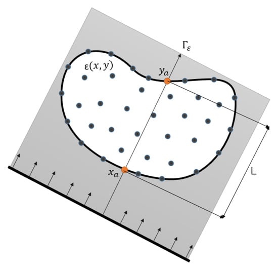
Figure 1. Coordinate system and geometry of Longitudinal Ray transform with the node set.

3. Meshless Approach Overview

One of the most common techniques among meshfree methods is the Radial Basis Functions (rbf). The formal definition of a radial function is given below.

Definition 1.

A function $\mathsf{\Phi }:R^d\times R^d\to R$ is called radial provided there exists a univariate function $\psi :[0,\infty ]\to R$ such that $\mathsf{\Phi }(\mathbf{x}-\mathbf{y})=\psi (r)$, where $r=\parallel \mathbf{x}-\mathbf{y}\parallel$, where we choose $\parallel ·\parallel$ to be the Euclidean norm on $R^d$.

The proposed approach is similar to the three-layer feed-forward rbf neural network [29,30]. The first layer is the network inputs, the second a hidden layer consisting of a collection of nonlinear rbf activation units, and the third corresponds to the final network output. In Radial Basis Function Networks (rbfn), activation functions are usually implemented as Gaussian functions. An overview of rbfn structure is shown in Figure 2. To illustrate how the rbfn works, assume that we have a set of D data with N patterns of $(x_p,y_p)$ in which $x_p$ is the input of the set of data and $y_p$ is the actual output. The $i\mathrm{th}$ activation function in the hidden network layer can be determined from the gap between input pattern x and centers i based on Equation (2)

$${\varphi }_i(\parallel \mathbf{x}-{\mathbf{c}}_i\parallel )=exp\left(-{\displaystyle \frac{\parallel \mathbf{x}-{\mathbf{c}}_i{\parallel }^2}{r_i^2}}\right),$$

(2)

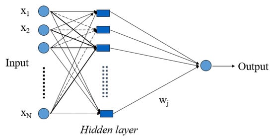
Figure 2. Radial basis function model network architecture.

Here, $\parallel ·\parallel$ is the Euclidean norm, $c_i$ and $r_i$ are the center and width of the hidden neuron i, respectively. Then the contribution of the k node from the network output layer can be computed with Equation (3)

$$y_k=\sum _{i=1}^n{w}_{ik}{\varphi }_i(\mathbf{x}).$$

(3)

3.1. Methodology

The addition of polynomials to the radial basis functions will ensure consistency and guarantees the approximation properties of the scheme. However, it complicates the system of equations making them difficult to enforce and contribute extra to computational cost and time. In the proposed method, $2\times 2$ symmetric strain tensor field $\epsilon (\mathbf{x})$ is composed of two parts: radial basis functions $R_i(\mathbf{x})$ and polynomial basis functions $P_j(\mathbf{x})$ [25,31]. Hence, the local approximation is given by

$${\epsilon }_{lk}(\mathbf{x})=\sum _{i=1}^n{a}_i{R}_i(\mathbf{x})+\sum _{j=1}^m{b}_j{P}_j(\mathbf{x}),l,k=\{1,2\},$$

(4)

where m is the number of polynomial terms and n is the number of nodes in the local support domain $\mathsf{\Omega }$. Unknown vectors to be calculated are a and b. The addition of polynomial terms is an additional prerequisite. The following conditions are generally imposed to ensure a unique approximation [32]

$$\sum _{i=1}^n{P}_j({\mathbf{x}}_i)b_i=0,j=1,2,\dots ,m,$$

(5)

where m is a number of augmented multivariate polynomial basis functions, see Table A1. We assume $P_j(\mathbf{x})=1+x+y+xy+x^2+y^2$ and $R_i(\mathbf{x})=exp(-{\alpha }^2\parallel \mathbf{x}-{\mathbf{c}}_i{\parallel }^2)$ where $\alpha$ is the shaping parameter. Hence, above Equation (4) is expressed in the matrix form

$$U=R\mathbf{a}+P\mathbf{b},$$

(6)

where U is the vector of function values: $U={[{\epsilon }_{lk}^1,{\epsilon }_{lk}^2,\cdots ,{\epsilon }_{lk}^n]}^T$, R is the matrix of rbfs, P is the matrix of polynomial basis function and $\mathbf{a},\mathbf{b}$ are the values of unknown coefficients (Radial and polynomial respectively). We note that to obtain the unique solution of Equation (4), the constraint condition (5) should be combined with Equation (6) as follows

$$U_1=\left[\begin{array}{c}U\\ 0\end{array}\right]=\left[\begin{array}{cc}R& P\\ P^T& 0\end{array}\right]\left[\begin{array}{c}\mathbf{a}\\ \mathbf{b}\end{array}\right]=F{\mathbf{a}}_{\mathbf{0}},$$

(7)

The unknown vector in Equation (7) is obtained by the inversion of the matrix $F=\left[\begin{array}{cc}R& P\\ P^T& 0\end{array}\right].$

3.1.1. Weak Form for Longitudinal Ray Transform Integral

Let us consider a two-dimension strain reconstruction problem in domain $\mathsf{\Omega }$ whose strong form is given by Equation (1) and generalized weak form is obtained as

$${\mathsf{\Gamma }}_{\epsilon }=\frac{1}{L}{\int }_0^L{n}_1^2{\epsilon }_{11}+2n_1{n}_2{\epsilon }_{12}+n_2^2{\epsilon }_{22}ds,$$

(8)

Enforcing (8) to pass through all node values in the domain $\mathsf{\Omega }$, the following equations are obtained

$$CU=\mathsf{\Gamma },$$

(9)

where C is the coefficient matrix; U is the vector of unknowns and $\mathsf{\Gamma }$ is the vector of integral values. Now, rewriting (4) in a matrix form to find weights

$$\left[\begin{array}{cc}{(A)}_{N\times N}& {(P)}_{N\times 3}\\ {(P^T)}_{3\times N}& {(0)}_{3\times 3}\end{array}\right]\left[\begin{array}{c}{(U_1)}_{N\times 1}\\ {(U_2)}_{3\times 1}\end{array}\right]=\left[\begin{array}{c}{({\epsilon }_{11}(x_i,y_i))}_{N\times 1}\\ {(0)}_{3\times 1}\end{array}\right],$$

$$\left[\begin{array}{cc}{(A)}_{N\times N}& {(P)}_{N\times 3}\\ {(P^T)}_{3\times N}& {(0)}_{3\times 3}\end{array}\right]\left[\begin{array}{c}{(V_1)}_{N\times 1}\\ {(V_2)}_{3\times 1}\end{array}\right]=\left[\begin{array}{c}{({\epsilon }_{12}(x_i,y_i))}_{N\times 1}\\ {(0)}_{3\times 1}\end{array}\right],$$

$$\left[\begin{array}{cc}{(A)}_{N\times N}& {(P)}_{N\times 3}\\ {(P^T)}_{3\times N}& {(0)}_{3\times 3}\end{array}\right]\left[\begin{array}{c}{(W_1)}_{N\times 1}\\ {(W_2)}_{3\times 1}\end{array}\right]=\left[\begin{array}{c}{({\epsilon }_{22}(x_i,y_i))}_{N\times 1}\\ {(0)}_{3\times 1}\end{array}\right],$$

(10)

where N is the total number of nodes in the domain $\mathsf{\Omega }$,

$$A=\left[\begin{array}{cccc}\varphi (\parallel {\mathbf{x}}_1,{\mathbf{x}}_1\parallel )& \varphi (\parallel {\mathbf{x}}_1,{\mathbf{x}}_2\parallel )& \cdots & \varphi (\parallel {\mathbf{x}}_1,{\mathbf{x}}_N\parallel )\\ \varphi (\parallel {\mathbf{x}}_2,{\mathbf{x}}_1\parallel )& \varphi (\parallel {\mathbf{x}}_2,{\mathbf{x}}_2\parallel )& \cdots & \varphi (\parallel {\mathbf{x}}_2,{\mathbf{x}}_N\parallel )\\ ⋮& ⋮& & ⋮\\ \varphi (\parallel {\mathbf{x}}_N,{\mathbf{x}}_1\parallel )& \varphi (\parallel {\mathbf{x}}_n,{\mathbf{x}}_2\parallel )& \cdots & \varphi (\parallel {\mathbf{x}}_n,{\mathbf{x}}_N\parallel )\end{array}\right],$$

(11)

$${({\epsilon }_{lk}(x_i,y_i))}_{N\times 1}={({\epsilon }_{lk}(x_1,y_1),{\epsilon }_{lk}(x_2,y_2),\dots ,{\epsilon }_{lk}(x_N,y_N))}^T,l,k=1,2,$$

(12)

and

$$P=\left[\begin{array}{ccccc}1& x_1& y_1& \cdots & P_m(x_1,y_1)\\ 1& x_2& y_2& \cdots & P_m(x_2,y_2)\\ ⋮& & ⋮& & ⋮\\ 1& x_N& y_N& \cdots & P_m(x_N,y_N)\end{array}\right].$$

(13)

Hence,

$$\left[\begin{array}{c}{(U_1)}_{N\times 1}\\ {(U_2)}_{3\times 1}\end{array}\right]={\left[\begin{array}{cc}{(A)}_{N\times N}& {(P)}_{N\times 3}\\ {(P^T)}_{3\times N}& {(0)}_{3\times 3}\end{array}\right]}^{-1}\left[\begin{array}{c}{({\epsilon }_{11}(x_i,y_i))}_{N\times 1}\\ {(0)}_{3\times 1}\end{array}\right]$$

(14)

$$\left[\begin{array}{c}{(V_1)}_{N\times 1}\\ {(V_2)}_{3\times 1}\end{array}\right]={\left[\begin{array}{cc}{(A)}_{N\times N}& {(P)}_{N\times 3}\\ {(P^T)}_{3\times N}& {(0)}_{3\times 3}\end{array}\right]}^{-1}\left[\begin{array}{c}{({\epsilon }_{12}(x_i,y_i))}_{N\times 1}\\ {(0)}_{3\times 1}\end{array}\right]$$

(15)

$$\left[\begin{array}{c}{(W_1)}_{N\times 1}\\ {(W_2)}_{3\times 1}\end{array}\right]={\left[\begin{array}{cc}{(A)}_{N\times N}& {(P)}_{N\times 3}\\ {(P^T)}_{3\times N}& {(0)}_{3\times 3}\end{array}\right]}^{-1}\left[\begin{array}{c}{({\epsilon }_{22}(x_i,y_i))}_{N\times 1}\\ {(0)}_{3\times 1}\end{array}\right]$$

(16)

and

$$U={[{(U_1)}_{N\times 1},{(U_2)}_{3\times 1},{(V_1)}_{N\times 1},{(V_2)}_{3\times 1},{(W_1)}_{N\times 1},{(W_2)}_{3\times 1}]}^T$$

(17)

Now, using Equations (14)–(17) in the previous system (9), we get

$$B\epsilon =\mathsf{\Gamma },$$

(18)

which lead to an optimization problem as follows

$${min\parallel B\epsilon -\mathsf{\Gamma }\parallel }_2.$$

(19)

To ensure uniqueness, equilibrium equations are imposed as follows:

$$\underset{\mathsf{\Omega }}{\int \int }\left(\frac{\partial }{\partial x}({\epsilon }_{11}+\nu {\epsilon }_{22})+\frac{\partial }{\partial y}(1-\nu ){\epsilon }_{12}\right)R_i(x)=0,i=1,2,\dots ,n,$$

(20)

$$\underset{\mathsf{\Omega }}{\int \int }\left(\frac{\partial }{\partial y}({\epsilon }_{22}+\nu {\epsilon }_{11})+\frac{\partial }{\partial x}(1-\nu ){\epsilon }_{12}\right)R_i(x)=0,i=1,2,\dots ,n,$$

(21)

This will give us another system of equations

$$C\epsilon =0.$$

(22)

The least square algorithm, described in [33], is well suited to this task. In general, least square computes a solution $\epsilon$ to problems of the following form

$$\underset{C\epsilon =0}{min}{\parallel B\epsilon -\mathsf{\Gamma }\parallel }_2,$$

(23)

which is solved using least square optimization intrinsic function “lsqlin” in matlab.

3.1.2. Shape Parameter

For the precise implementation of the framework, the shape parameter evaluation is important [34]. Therefore, careful attention should be given for determining shape parameter value. Detailed discussions regarding values for the shape parameter can be found in Fasshauer [35], Franke [36], and Hardy [37]. Most formulations for shape parameters depend on the distance, d, and node numbers, N. Other formulations display a changing shape parameter depending on the location of the node. In general, the shape parameter depends upon several variables such as the data point distribution, the basis function, and a computer precision (see [38]). The effect of the rbf Gaussian shaping parameter $\alpha$ mentioned above is shown in Figure 3.

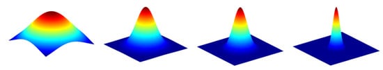
Figure 3. Effect of Shaping Parameter for $\alpha =$1, 5 10, and 40, respectively.

3.1.3. Algorithm

Here, we discuss the difference between two methods; namely fem and rbf. Detailed pseudo-code algorithm is given below Algorithms 1 and 2 for both the methods, respectively.

Algorithm 1: Pseudo-Code for the fem algorithm

Algorithm 2: Pseudo-Code for the proposed rbf algorithm

The complicated meshing rules are not required while performing rbf, and here lies the advantage of the proposed method over the framework of finite elements. The use of meshless methods over the finite-element approach for reconstruction tensor strain field [39,40,41] has many other benefits. We can quickly increase the support domain, change basis functions, adopt nodal densities, and many more. Those characteristics can be useful in the case of irregularities like sharp discontinuations or other situations in complex simulations. In the next section, we talk about this difference between methods with a simulated example.

4. Cantilevered Beam

Here we illustrate the practical performance of the proposed algorithm, starting with the well-known two-dimensional cantilevered beam problem that was previously successfully determined by other authors [9]. In this case, we take the $[0,20]\times [-5,5]$ a two-dimensional strain domain into account with a 2 kN load over the beam. The beam’s material properties reflect common steel, while other parameters are listed below.

The data consist of 9 projections evenly spaced in ${[0,170]}^{\circ }$ with 200 lines each, yielding a total of 1800 measurements. Figure 4 shows two types of nodal mesh (uniform and non-uniform) used for beam strain field reconstruction using rbf. Both nodal mesh consist of 400 nodes including boundary points. Figure 5 shows the reconstruction of strain field using rbf, whereas Figure 6 shows the analytical solution of the cantilevered beam. The plane stress Saint-Venant approximation to the strain field is [42]:

$${\epsilon }_{xx}=\frac{P(L-x)y}{EI},{\epsilon }_{xy}=-\frac{(1+\nu )P}{2EI}\left(\frac{h^2}{y}-y^2\right),{\epsilon }_{yy}=-\frac{\nu P(L-x)y}{EI},$$

where I represents the second moment of area, L the beam length, h the beam height, t is the thickness, E is Young’s modulus, $\nu$ is the Poisson ratio, and the dimensions are shown in Table A2.

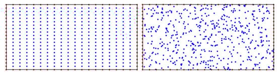
Figure 4. Uniform node set containing $N=400$ versus non-uniform nodal domain containing $N=400$ randomly spaced nodes.

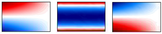
Figure 5. rbf Beam solution (Reconstructed solution ${\epsilon }_{xx},{\epsilon }_{xy},{\epsilon }_{yy}$).

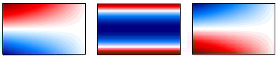
Figure 6. Beam solution (True solution ${\epsilon }_{xx},{\epsilon }_{xy},{\epsilon }_{yy}$).

Error Analysis through Simulation Results for rbf Methods

A $L^2$ error analysis of strain field associated with both fem and rbf methods is shown in Figure 7. Started with 9 projections evenly spaced in ${[0,170]}^{\circ }$ with 10 lines each and ended with 700 lines each 9 projections. Both rbf case results shows better agreement than fem in the final stage. However, faster convergence is seen in the case of uniform rbf. Figure 8 shows the rms error between the reconstructed and analytical strain field as we change Gaussian function shaping parameter value.

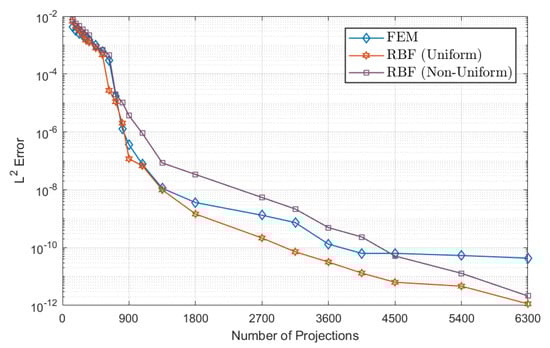
Figure 7. $L^2$ error.

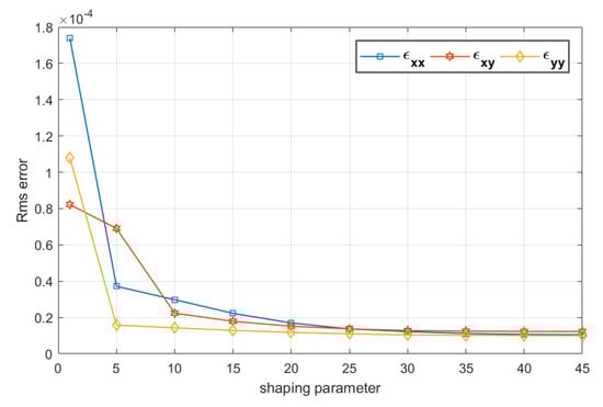
Figure 8. Rms error.

The numerical rms error with different shaping parameter values are calculated using the root-mean-square error and shown in Figure 8

$$\mathrm{Error}=\sqrt{{\displaystyle \frac{{\sum }_{i=1}^N{(T_i-R_i)}^2}{N}}},$$

where N is the total number of nodes, $T_i$ is the true strain value and $R_i$ is the reconstructed strain value at the particular node i. We found out the proposed reconstruction algorithm extremely useful for the reconstruction of the strain field. The simulation results imply that the reconstruction algorithm will converge to an appropriate reconstruction provided measurements over ${180}^{\circ }$ of a sample are calculated. Discretization problems and numerical errors will undoubtedly lead to noisy reconstruction. As the number of projections increased, rapid convergence to the analytic solution was observed. The constrained optimization problem (23) can be solved using a variety of approaches. Our algorithm uses the “lsqlin” inbuild function in MATLAB. This convergence gives us confidence that in the face of real experimental uncertainties, the algorithm will converge to an analytic solution.

5. Experimental Demonstration

The rbf approximation methods presented above have been tested on synthetic and real data sets. We are now testing the algorithm on the experimental data previously studied for the offset ring-and-plug, and the crushed ring sample [26]. The crushed ring sample was 14 mm thick with 23 mm outer diameter and, 10 mm inner diameter. To test the algorithm for continuous and discontinuous stress fields, specific samples were selected. The ring-and-plug sample is designed to test the discontinuous strain field and the crushed ring for continuous strain field testing. The offset ring-and-plug sample geometry is shown in Figure 9, and the crushed ring is shown on the left side of Figure 10. The sample described included a total interference of $40\pm 2\mathsf{\mu }$m generated by cylindrical grinding. Although the plastic deformation of the crushed ring sample by 1.5 mm on the diameter was achieved using 8.4 kN rigid steel plates. A brief description of the model and experimental settings is provided below and can be found in [26]. Two EN26 steel bars have been heated to relieve stress and provide a uniform structure before assembly. The final test hardness of the sample was 290 HV for both models. The strain profile was calculated on raden along with an MCP detector (512 × 512 pixels, $55\mathsf{\mu }$m per pixel) at 17.9 m from the beam source of power 409 kW (January 2018). In the Japan Proton Accelerator Research Complex j-parc, Japan, the neutron-energy-resolved imaging instrument was used to obtain the relative shifts of the Bragg edges corresponding to the lattice plane of the samples. Neutron strain scanning was performed on kowari, a residual stress diffractometer at the Australian Nuclear Society and Technology Organization (ansto), Australia, to verify our reconstruction independently. This strain-scan provide measurements of the three in-plane components of strain over a mesh of points within the sample using a $0.5\times 0.5\times 14$ mm gauge volume. Sampling times on kowari were based on the providing of strain uncertainty around $7\times {10}^{-5}$, which required about 30 h of beam time per component. The raden sampling times, however, were based on the $1\times {10}^{-4}$ statistical uncertainty. A total of 50 profiles were measured at golden angle increments in the angle with a sampling time of two hours per projection.

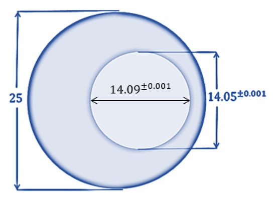
Figure 9. Offset-Ring-and-Plug sample geometry.

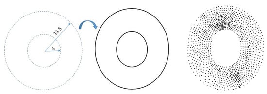
Figure 10. Crushed Ring Sample. The figure on the left shows the sample geometry for crushed ring steel sample before and after applying force (all dimensions are in mm). The figure on the right shows a node set containing $N=$ non-uniform spaced nodes on the crushed ring sample.

A two-dimensional scattered data point net is used to discretize the domain of the sample, as shown in Figure 9. Two different types of node discretization have been considered: uniform and non-uniform (random). Nodal set can be seen in Figure 11 and reconstructed strain fields can be seen with each discretization in Figure 12 and Figure 13 respectively. As stated earlier, for the simulated problem, the reconstructed strain field did contain noise which can be from either experimental measurement or numerical discretizations.

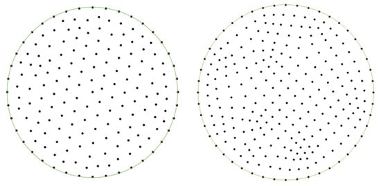
Figure 11. Offset-Ring-and-Plug Sample. The figure on the left shows a uniform data points set containing $N=260$. The figure on the right shows a scattered data points set containing $N=261$ non-uniform spaced nodes on the sample geometry.

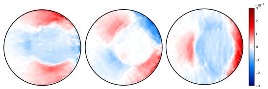
Figure 12. The reconstructed full-field two-dimensional strain components (${\epsilon }_{xx},{\epsilon }_{xy}$, and ${\epsilon }_{yy}$) with non-uniform node distribution.

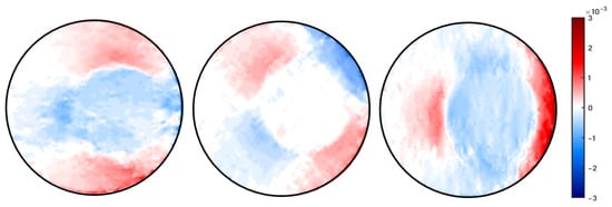
Figure 13. The reconstructed full-field two-dimensional strain components (${\epsilon }_{xx},{\epsilon }_{xy}$, and ${\epsilon }_{yy}$) with uniform node distribution.

To summarize, we proposed a meshless approach using rbf. They are the natural generalization in a multivariate sense of univariate polynomial splines. It works well for high-dimensional arbitrary structures, and no mesh requirement is the main benefit of this form of approximation. A rbf is a function, the value of which depends only on the distance between the points. Due to the use of distance functions, one can conveniently deploy rbfs to recreate the surface using data points in 2d, 3d or higher-dimensional spaces.

The Least square solution was found for 3790 nodes for the non-uniform and 3795 nodes for uniform ring-and-plug discretization from 22,678 projections. Figure 12 and Figure 13 shows the reconstructed field of ring-and-plug with uniform and non-uniform node distribution respectively in terms of three Cartesian strain components namely; ${\epsilon }_{xx},{\epsilon }_{xy}$ and ${\epsilon }_{yy}$. The reconstructed strain field was found for 1352 nodes and 1086 quadrilateral elements via fem approach and 1352 nodes for crushed ring discretization via rbf approach from 20,664 projections. Figure 14 and Figure 15 shows the reconstructed strain field of crushed ring with fem and rbf respectively in terms of three Cartesian strain components. Figure 16 and Figure 17 show the corresponding validated strain field from kowari data. The effectiveness of the suggested approach is not based solely on sample structures and can, thus, be extended to three-dimensional sample bodies. Due to radial basis function computation, the real challenge is the computational cost and time since the size of the problem is quite large.

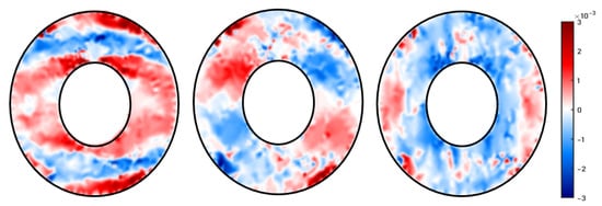
Figure 14. The reconstructed full-field two-dimensional strain components (${\epsilon }_{xx},{\epsilon }_{xy}$, and ${\epsilon }_{yy}$) with fem.

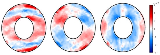
Figure 15. The reconstructed full-field two-dimensional strain components (${\epsilon }_{xx},{\epsilon }_{xy}$, and ${\epsilon }_{yy}$) with rbf.

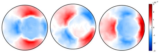
Figure 16. Two-dimensional strain components ${\epsilon }_{xx},{\epsilon }_{xy},{\epsilon }_{yy}$ respectively with kowari Data.

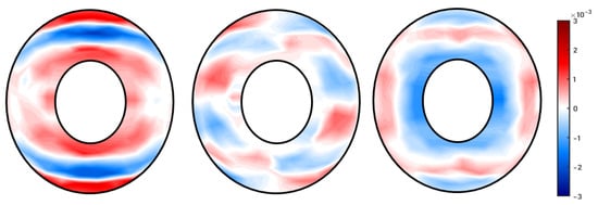
Figure 17. Two-dimensional strain components ${\epsilon }_{xx},{\epsilon }_{xy},{\epsilon }_{yy}$ respectively with kowari Data.

6. Conclusions

From Bragg-edge neutron images, an elastic strain tensor field reconstruction algorithm has been presented. Unlike previous algorithms such as fem, our suggested methodology is capable of reconstructing residual strain field as no elastic strain compatibility is assumed. Simulated and experimental data from kowari and raden have shown this process. The analysis revealed a strong agreement with the strain maps measured using the constant diffractometer Kowari. A complete strain field tomography can now be achieved using physical constraints as an equilibrium without thinking about two-dimensional mesh. This approach opens up more study, including three dimensions, for future studies. The framework taken allows us to concentrate on the highly stressed region of the sample using adaptive node discretization, which can be accomplished by calculating the gradient over the sample.

Appendix A.1. Polynomial Basis Functions

Table A1. Number of polynomial terms based on the degree of polynomial.

Polynomial Degree (${\mathit{P}}_{\mathit{d}}$)	Polynomial Basis	$\mathit{m}={\displaystyle \frac{({\mathit{P}}_{\mathit{d}}+2)!}{2!{\mathit{P}}_{\mathit{d}}!}}$
0	1	1
1	$1,x,y$	3
2	$1,x,y,x^2,y^2,xy$	6
3	$1,x,y,x^2,y^2,xy,x^{2}y,x{y}^2,x^3,y^3$	10
4	⋯	15
⋮	⋮	⋮

Table A1. Number of polynomial terms based on the degree of polynomial.

Polynomial Degree (${\mathit{P}}_{\mathit{d}}$)	Polynomial Basis	$\mathit{m}={\displaystyle \frac{({\mathit{P}}_{\mathit{d}}+2)!}{2!{\mathit{P}}_{\mathit{d}}!}}$
0	1	1
1	$1,x,y$	3
2	$1,x,y,x^2,y^2,xy$	6
3	$1,x,y,x^2,y^2,xy,x^{2}y,x{y}^2,x^3,y^3$	10
4	⋯	15
⋮	⋮	⋮

Appendix A.2. Parameter Used for Cantilevered Beam Simulation

Table A2. Beam Problem Parameters.

Parameter	Symbol	Value
Young’s Modulus	E	200 GPa
Edge Load	P	2 kN
Beam Length	L	12 mm
Beam height	W	10 mm
Beam thickness	t	3 mm
Poisson’s ratio	$\nu$	0.3

Table A2. Beam Problem Parameters.

Parameter	Symbol	Value
Young’s Modulus	E	200 GPa
Edge Load	P	2 kN
Beam Length	L	12 mm
Beam height	W	10 mm
Beam thickness	t	3 mm
Poisson’s ratio	$\nu$	0.3

References

- Boothroyd, A. Principles of Neutron Scattering from Condensed Matter; Oxford University Press: Oxford, UK, 2020. [Google Scholar]
- Schelten, J.; Ballard, D.G.H.; Wignall, G.D.; Longman, G.; Schmatz, W. Small-angle neutron scattering studies of molten and crystalline polyethylene. Polymer 1976, 17, 751–757. [Google Scholar] [CrossRef]
- Santisteban, J.R.; Edwards, L.; Fizpatrick, M.E.; Steuwer, A.; Withers, P.J. Engineering applications of Bragg-edge neutron transmission. Appl. Phys. A 2002, 74, 1433–1436. [Google Scholar] [CrossRef]
- Song, G.; Lin, J.Y.; Bilheux, J.C.; Xie, Q.; Santodonato, L.J.; Molaison, J.J.; Skorpenske, H.D.; Santos, A.M.D.; Tulk, C.A.; An, K.; et al. Characterization of Crystallographic Structures Using Bragg-Edge Neutron Imaging at the Spallation Neutron Source. J. Imaging 2017, 3, 65. [Google Scholar] [CrossRef]
- Gregg, A.; Hendriks, J.N.; Wensrich, C.; Meylan, M.H. Tomographic reconstruction of residual strain in axisymmetric systems from Bragg-edge neutron imaging. Mech. Res. Commun. 2017, 85, 96–103. [Google Scholar] [CrossRef]
- Abbey, B.; Zhang, S.Y.; Vorster, W.J.J.; Korsunsky, A.M. Feasibility study of neutron strain tomography. Procedia Eng. 2009, 1, 185–188. [Google Scholar] [CrossRef]
- Lionheart, W.R.B.; Withers, P.J. Diffraction tomography of strain. Inverse Probl. 2015, 31, 045005. [Google Scholar] [CrossRef]
- Hammer, H.; Lionheart, B. Application of Sharafutdinov’s ray transform in integrated photoelasticity. J. Elast. 2004, 75, 229–246. [Google Scholar] [CrossRef]
- Wensrich, C.; Hendriks, J.; Gregg, A.; Meylan, M.; Luzin, V.; Tremsin, A. Bragg-edge neutron transmission strain tomography for in situ loadings. Nucl. Instrum. Methods Phys. Res. B 2016, 383, 52–58. [Google Scholar] [CrossRef]
- Hendriks, J.N.; Gregg, A.W.T.; Wensrich, C.M.; Tremsin, A.S.; Shinohara, T.; Meylan, M.; Kisi, E.H.; Luzin, V.; Kirsten, O. Bragg-edge elastic strain tomography for in situ systems from energy-resolved neutron transmission imaging. Phys. Rev. Mater. 2017, 1, 053802. [Google Scholar] [CrossRef]
- Santisteban, J.; Edwards, L.; Fitzpatrick, M.; Steuwer, A.; Withers, P.; Daymond, M.; Johnson, M.; Rhodes, N.; Schooneveld, E. Strain Imaging by Bragg-edge neutron transmission. Nucl. Instrum. Methods Phys. Res. A 2002, 481, 765–768. [Google Scholar] [CrossRef]
- Kardjilov, N.; Manke, I.; Woracek, R.; Hilger, A.; Banhart, J. Advances in Neutron Imaging. Mater. Today 2018, 21, 652–672. [Google Scholar] [CrossRef]
- Sato, H.; Iwase, K.; Kamiyama, T.; Kiyanagi, Y. Simultaneous Broadening Analysis of Multiple Bragg Edges Observed by Wavelength-resolved Neutron Transmission Imaging of Deformed Low-carbon Ferritic Steel. ISIJ Int. 2020, 60, 1254–1263. [Google Scholar] [CrossRef]
- Tremsin, A.; McPhate, J.; Vallerga, J.; Siegmund, O.; Feller, W.; Lehmann, E.; Dawson, M. Improved efficiency of high resolution thermal and cold neutron imaging. Nucl. Instrum. Methods Phys. Res. A 2011, 628, 415–418. [Google Scholar] [CrossRef]
- Tremsin, A.S.; McPhate, J.B.; Kockelmann, W.; Vallerga, J.V.; Siegmund, O.H.W.; Feller, W.B. High resolution Bragg edge transmission spectroscopy at pulsed neutron sources: Proof of principle experiments with a neutron counting MCP detector. Nucl. Instrum. Methods Phys. Res. A 2011, 633, 235–238. [Google Scholar] [CrossRef]
- Tremsin, A.; McPhate, J.; Steuwer, A.; Kockelmann, W.; Paradowska, A.M.; Kelleher, J.; Vallerga, J.; Siegmund, O.; Feller, W. High-resolution strain mapping through time-of-flight neutron transmission diffraction with a microchannel plate neutron counting detector. Strain 2012, 48, 296–305. [Google Scholar] [CrossRef]
- Kirkwood, H.J.; Zhang, S.Y.; Tremsin, A.S.; Korsunsky, A.M.; Baimpas, N.; Abbey, B. Neutron Strain Tomography using the Radon Transform. Mater. Today Proc. 2015, 2, S414–S423. [Google Scholar] [CrossRef]
- Srivastava, M.H.; Ahmad, H.; Ahmad, I.; Thounthong, P.; Khan, N.M. Numerical simulation of three-dimensional fractional-order convection-diffusion PDEs by a local meshless method. Therm. Sci. 2020, 210. [Google Scholar] [CrossRef]
- Ahmad, I.; Siraj-ul-Islama; Khaliq, A.Q.M. Local RBF method for multi-dimensional partial differential equations. Comput. Math. Appl. 2017, 74, 292–324. [Google Scholar] [CrossRef]
- Smith, G.D.; Smith, G.D.; Smith, G.D.S. Numerical Solution of Partial Differential Equations: Finite Difference Methods; Oxford University Press: Oxford, UK, 1985. [Google Scholar]
- Reddy, J.N. An Introduction to the Finite Element Method; McGraw-Hill: New York, NY, USA, 1993; pp. 199–226. [Google Scholar]
- Flyer, N.; Wright, G.B.; Fornberg, B. Radial basis function-generated finite differences: A mesh-free method for computational geosciences. In Handbook of Geomathematics; Springer: Berlin/Heidelberg, Germany, 2014; pp. 1–30. [Google Scholar]
- Fasshauer, G.E. Meshfree Approximation Methods with MATLAB; World Scientific: Singapore, 2007; Volume 6. [Google Scholar]
- Zhang, H.; Zhang, Y. Mesh-free method. In Deterministic Numerical Methods for Unstructured-Mesh Neutron Transport Calculation; Elsevier: Amsterdam, The Netherlands, 2004; pp. 215–242. [Google Scholar]
- Liu, G. An overview on meshfree methods: For computational solid mechanics. Int. J. Comput. Methods 2016, 13, 1630001. [Google Scholar] [CrossRef]
- Gregg, A.W.T.; Hendriks, J.N.; Wensrich, C.M.; Will, A.; Tremsin, A.S.; Luzin, V.; Shinohara, T.; Kirstein, O.; Meylan, M.H.; Kisi, E.H. Tomographic Reconstruction of Two-Dimensional Residual Strain Fields from Bragg-Edge Neutron Imaging. Phys. Rev. Appl. 2018, 10, 064034. [Google Scholar] [CrossRef]
- Jidling, C.; Hendriks, J.; Wahlström, N.; Gregg, A.; Schön, T.B.; Wensrich, C.; Wills, A. Probabilistic modelling and reconstruction of strain. Nucl. Instrum. Methods Phys. Res. B 2018, 436, 141–155. [Google Scholar] [CrossRef]
- Ramadhan, R.S.; Syed, A.K.; Tremsin, A.S.; Kockelmann, W.; Dalgliesht, R.; Chen, B.; Parfitt, D.; Fitzpatrick, M.E. Mapping residual strain induced by cold working and by laser shock peening using neutron transmission spectroscopy. Mater. Des. 2018, 143, 56–64. [Google Scholar] [CrossRef]
- Park, J.; Sandberg, I.W. Universal approximation using radial-basis-function networks. Neural Comput. 1991, 3, 246–257. [Google Scholar] [CrossRef] [PubMed]
- Orr, M.J. Introduction to Radial Basis Function Networks; University of Edinburgh: Edinburgh, UK, 1996. [Google Scholar]
- Majdisova, Z.; Skala, V. Radial basis function approximations: Comparison and applications. Appl. Math. Model. 2017, 51, 728–743. [Google Scholar] [CrossRef]
- Chandhini, G.; Sanyasiraju, Y. Local RBF-FD solutions for steady convection–diffusion problems. Int. J. Numer. Meth. Eng. 2007, 72, 352–378. [Google Scholar] [CrossRef]
- Paige, C.; Saunders, M. An Algorithm for Sparse Linear Equations and Sparse Least Squares: ACM Transactions in Mathematical Software, ACMSCU; ACM: New York, NY, USA, 1982. [Google Scholar]
- Koupaei, J.A.; Firouznia, M.; Hosseini, S.M.M. Finding a good shape parameter of RBF to solve PDEs based on the particle swarm optimization algorithm. Alex. Eng. J. 2018, 57, 3641–3652. [Google Scholar] [CrossRef]
- Fasshauer, G.E.; Zhang, J.G. On choosing “optimal” shape parameters for RBF approximation. Numer. Algorithms 2007, 45, 345–368. [Google Scholar] [CrossRef]
- Franke, R. Scattered data interpolation: Tests of some methods. Math. Comput. 1982, 38, 181–200. [Google Scholar]
- Hardy, R.L. Multiquadric equations of topography and other irregular surfaces. J. Geophys. Res. 1971, 76, 1905–1915. [Google Scholar] [CrossRef]
- Roque, C.; Ferreira, A.J. Numerical experiments on optimal shape parameters for radial basis functions. Numer. Methods Partial Differ. Equ. 2010, 26, 675–689. [Google Scholar] [CrossRef]
- Aggarwal, R.; Meylan, M.H.; Lamichhane, B.P.; Wensrich, C.M. Energy Resolved Neutron Imaging for Strain Reconstruction Using the Finite Element Method. J. Imaging 2020, 6, 13. [Google Scholar] [CrossRef]
- Aggarwal, R.; Lamichhane, B.; Meylan, M.; Wensrich, C. A comparison of triangular and quadrilateral finite element meshes for Bragg edge neutron transmission strain tomography. ANZIAM J. 2019, 61, C242–C254. [Google Scholar] [CrossRef]
- Aggarwal, R.; Meylan, M.; Lamichhane, B.; Wensrich, C. Finite element approach to Bragg edge neutron strain tomography. ANZIAM J. 2018, 60, C279–C294. [Google Scholar] [CrossRef]
- Beer, F.; Johnston, E.J.; DeWolf, J.; Mazurek, D. Mechanics of Materials; McGraw-Hill Science: Columbus, OH, USA, 2008. [Google Scholar]
Publisher’s Note: MDPI stays neutral with regard to jurisdictional claims in published maps and institutional affiliations. |
© 2021 by the authors. Licensee MDPI, Basel, Switzerland. This article is an open access article distributed under the terms and conditions of the Creative Commons Attribution (CC BY) license (http://creativecommons.org/licenses/by/4.0/).