MANTRA: An Effective System Based on Augmented Reality and Infrared Thermography for Industrial Maintenance

 ,
,  ,
,  ,
, 
Abstract
Featured Application
Abstract
1. Introduction
Proposals
- To our knowledge, it is the first time that an AR system has been used in combination with IRT in the field of industrial maintenance.
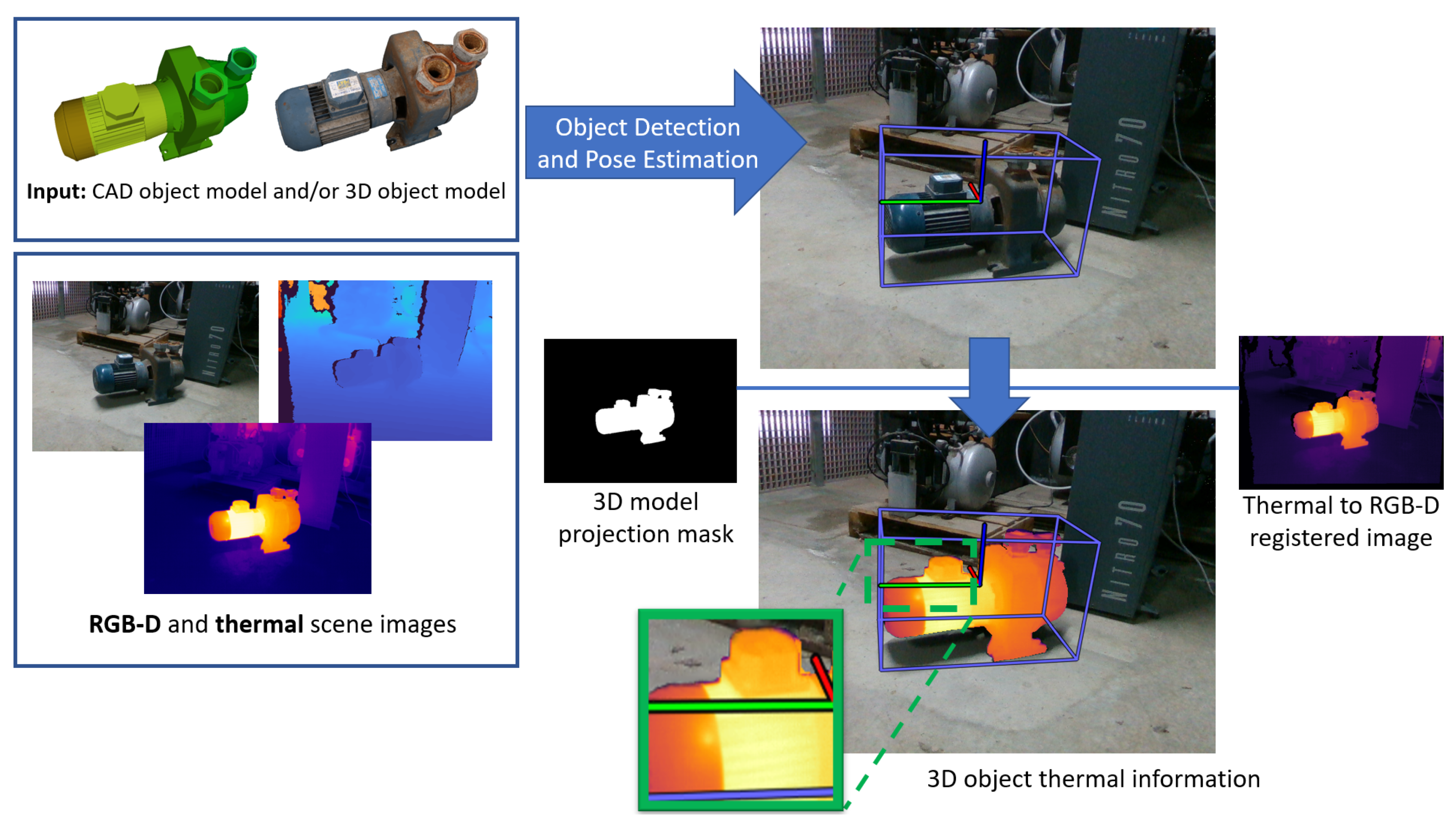
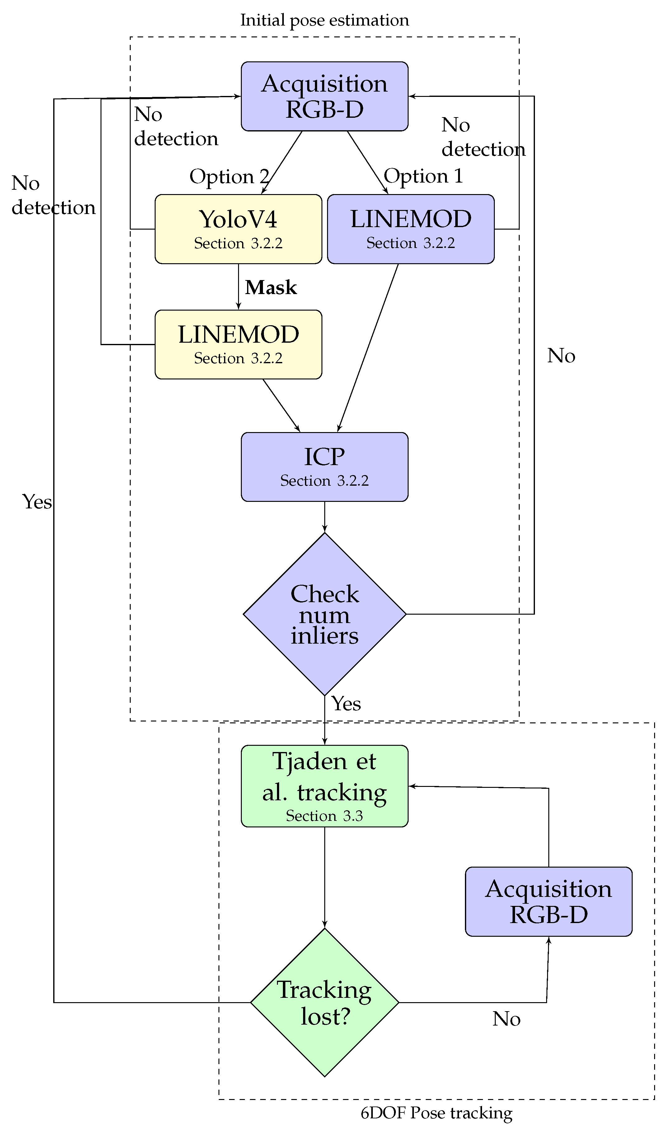
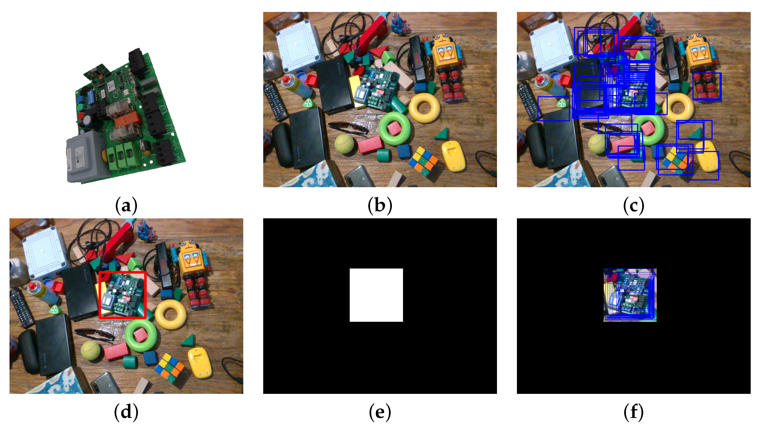
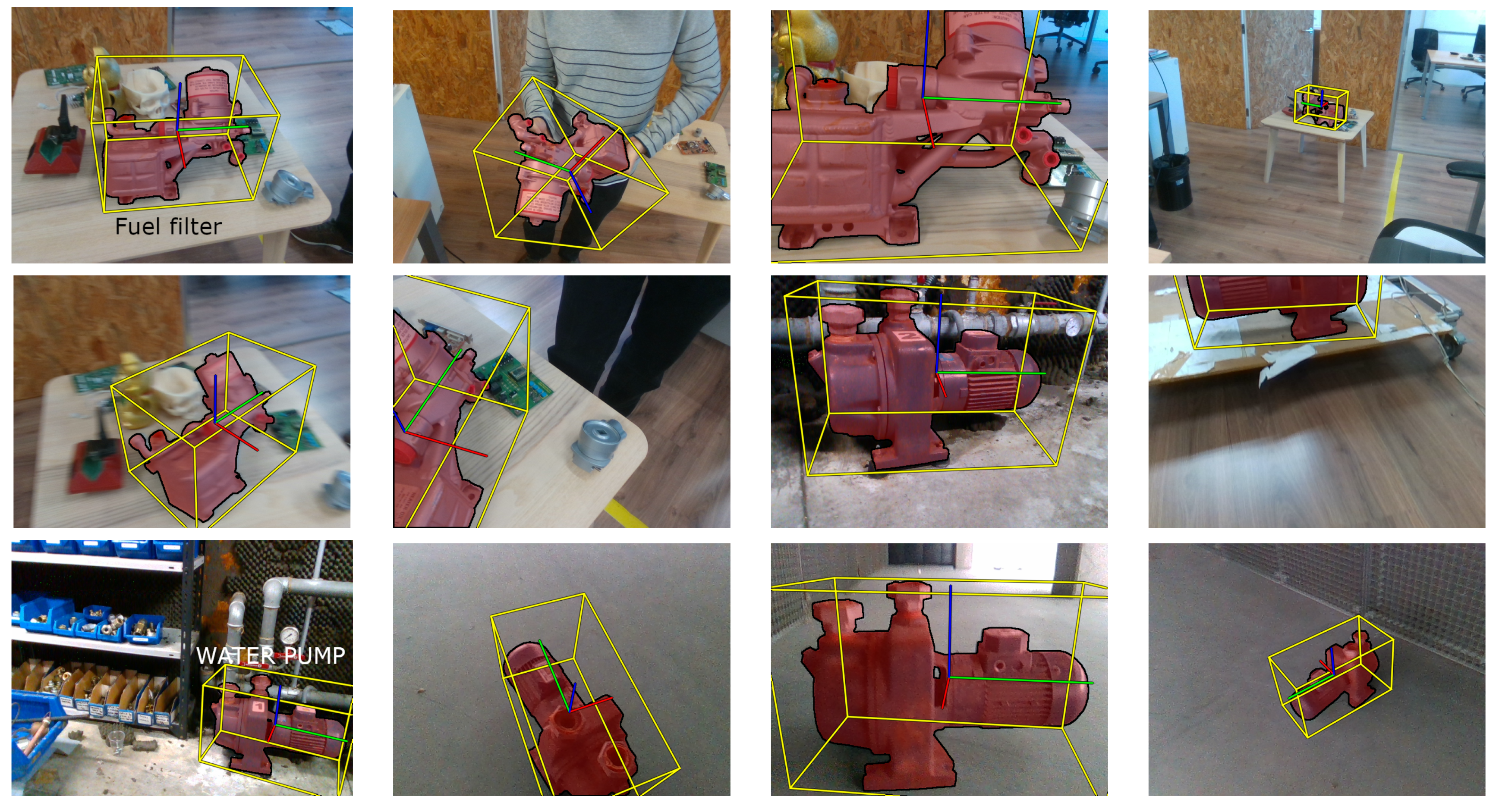
- We develop a new AR system using a combination of multiple methods that can align virtual content on 3D objects automatically, precisely, robustly, and in real time. Specifically, the 3D object detection and pose estimation method is based on a modified LINEMOD method [15] with a built-in deep-learning method called YOLOV4 [16]. In addition, a 6 Degree of Freedom (6DOF) pose tracking method, based on the work of Tjaden et al. [17], was also integrated. Finally, it is important to note that the YOLOV4 detection method was trained only with photorealistic synthetic images generated automatically by BlenderProc [18].
- The MANTRA system allows for obtaining the temperature information of a 3D object precisely and in real time, as well as that of its components, using the information of the previously calculated object pose.
- A new calibration pattern is designed, to spatially calibrate RGB-D and IRT cameras.
- The 3D object detection and pose estimation method used by the MANTRA system is validated on different public data sets.
- Both quantitative and qualitative validation of the MANTRA system, as applied to industrial maintenance in a real use-case, demonstrate its effectiveness, compared to traditional maintenance methods and those using only AR.
2. Related Work
3. Materials and Methods
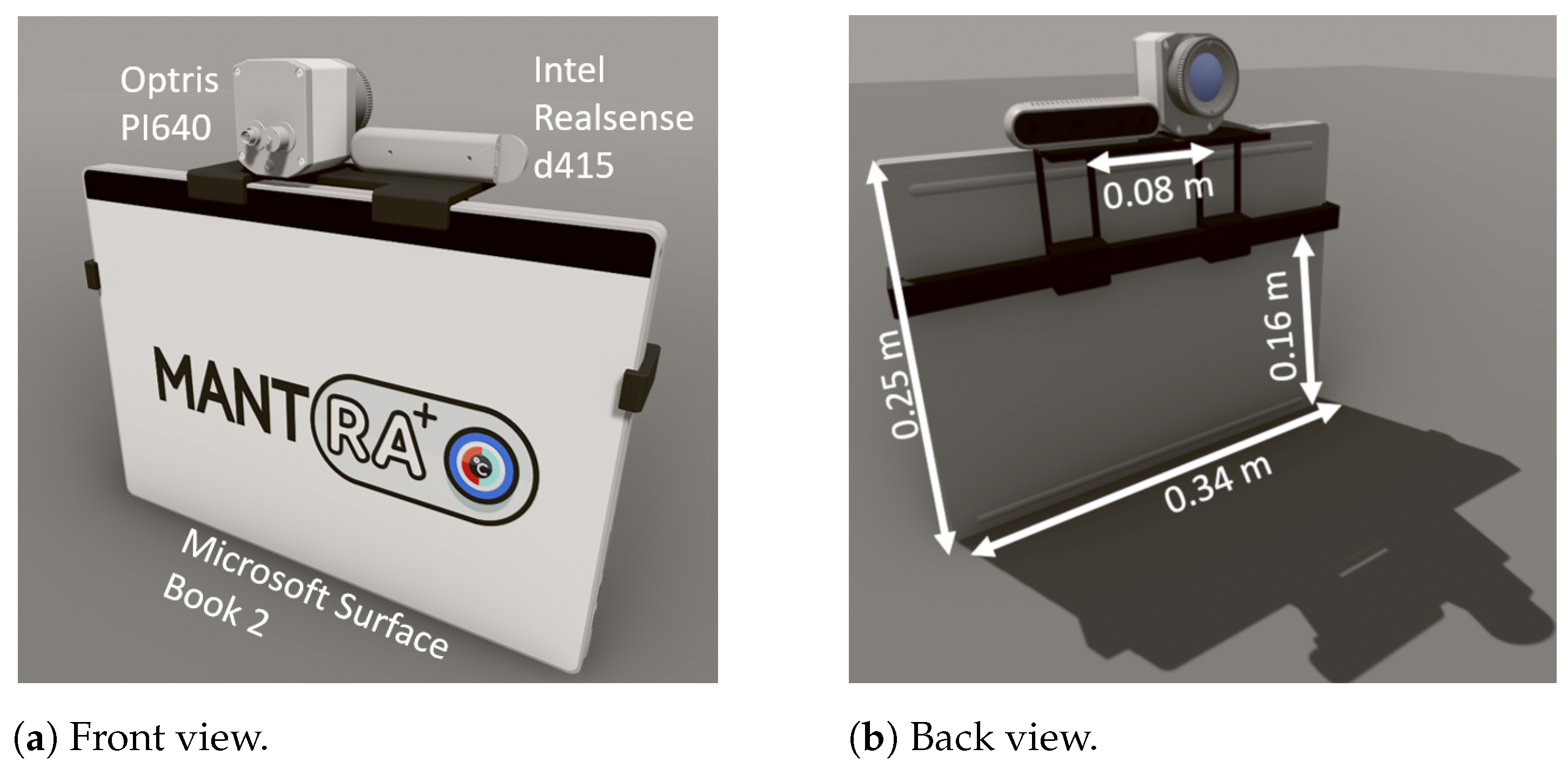
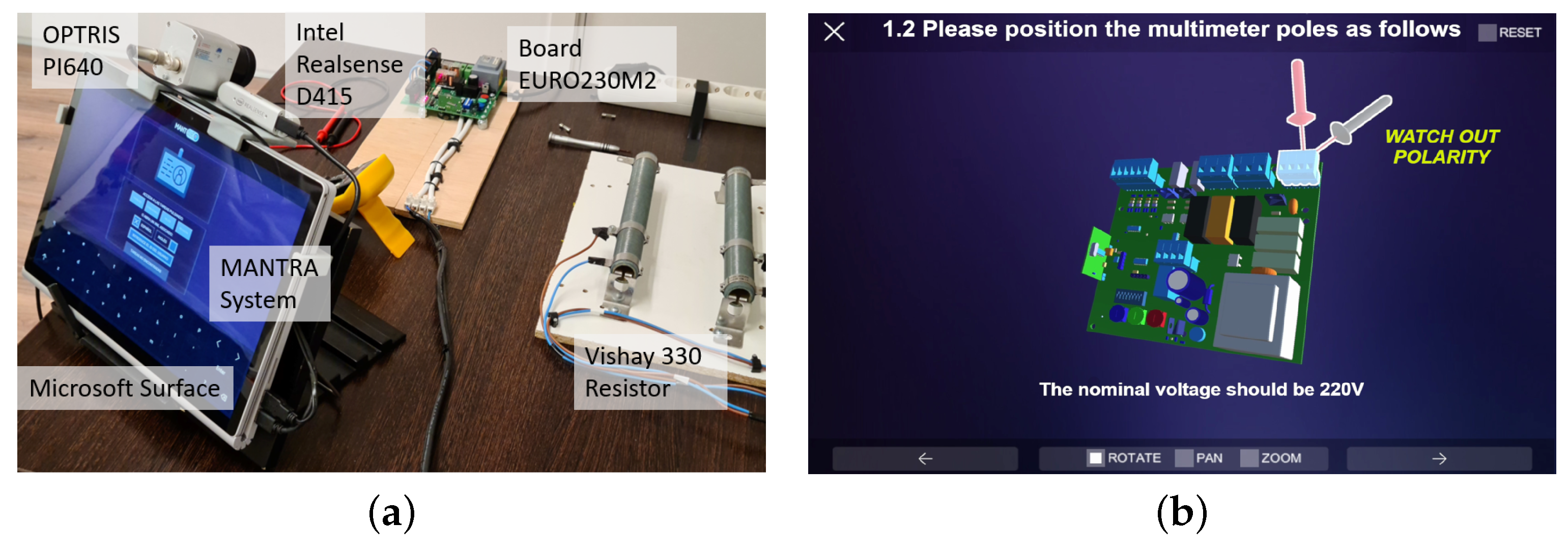
3.1. MANTRA System Description
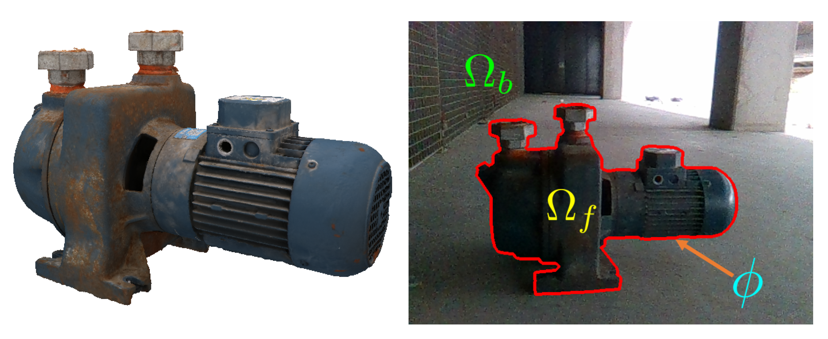
3.2. 3D Object Detection and Pose Estimation Module
3.2.1. Foundation
3.2.2. Method for Initial 3D Object Detection and Pose Estimation
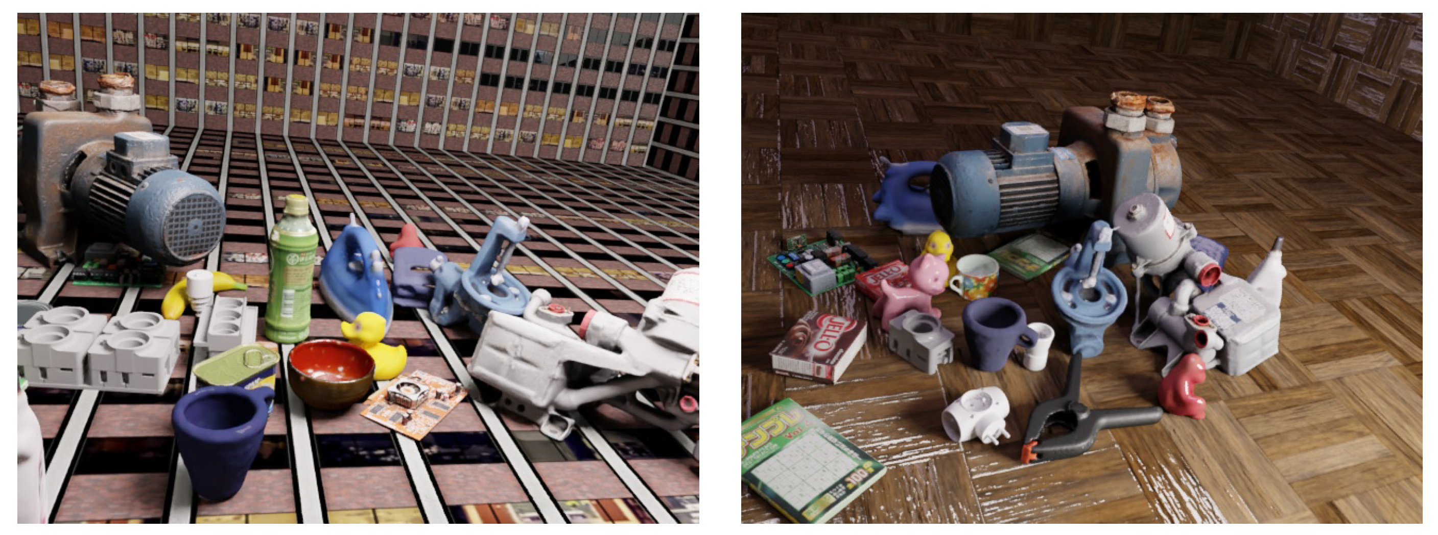
3.2.3. Training Detection Model
3.3. 6DOF Pose Tracking Module
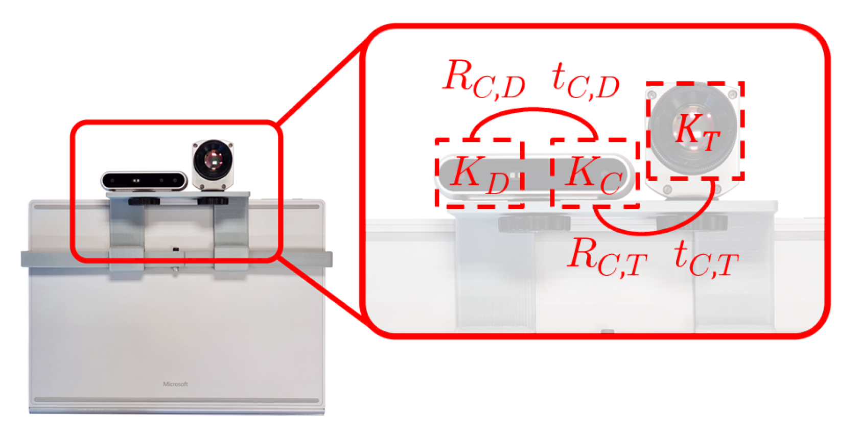
3.4. RGB-D and IRT Images Fusion Module
3.4.1. Sensor Calibration
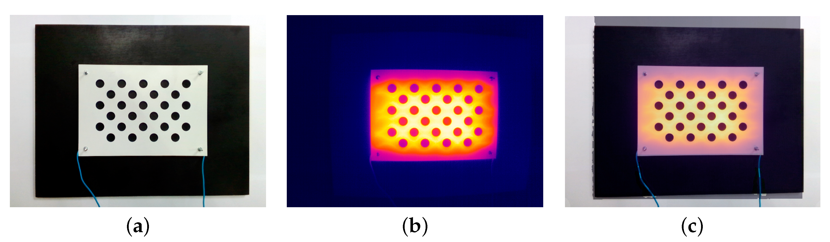
3.4.2. Calibration Target Used to Calibrate the IRT Camera
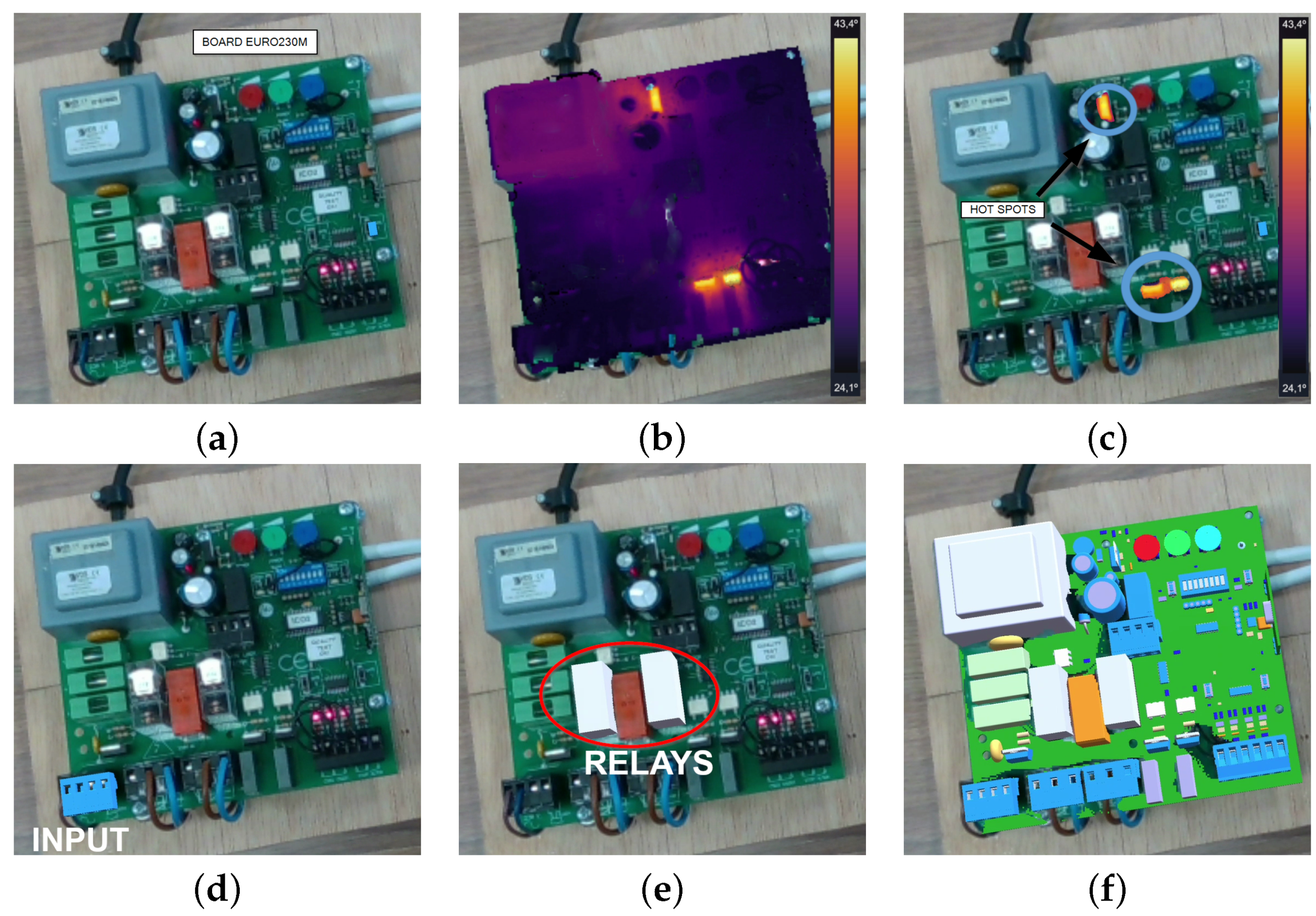
3.4.3. Thermal and RGB-D Image Fusion
4. Results
4.1. Quantitative Validation of the Results of the 3D Object Pose Detection and Estimation Method
4.2. Time Efficiency
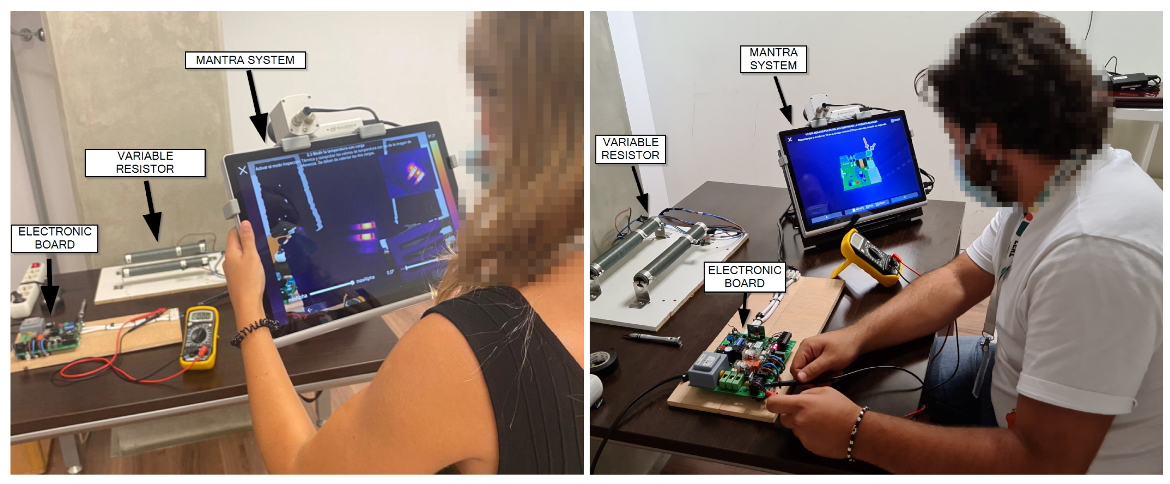
4.3. Maintenance Task Use-Case Efficiency Validation
- Reference state: This is the case where the electronic board works correctly. In this state, the board is programmed to complete the electromechanical process in 5 s by pressing the operation button.
- Blown fuse: This consists of the detection and replacement of one or more fuses on the board. To simulate this failure, a blown fuse was installed.
- Bad input connections: This occurs when a wire has come loose from the power input terminals or has burned out and does not conduct electricity.
- Relay malfunction: Relays control the activation of the outputs. If the mechanism is not making full contact or is stressed due to higher inrush current, carbon build-up can happen, due to excessive electrical arcing. This could lead to blockage, such that they cannot open or close the circuit.
- Bad contact in load outputs: This occurs when the wires have come loose from the output terminals and are not making good contact. This failure, which can lead to more severe failures and even lead to breakage of the device, consists of the appearance of bad contacts in the load connections where the different drives are powered.
- Overload/underload in the board drive: This fault occurs when the current to be supplied to the actuators is not as expected, which may be due to the interference of some type of external factor on the drive itself, which requires a higher power demand.
- Manual (M): This is the standard procedure, in which they have a manual, the equipment specification sheets, and an electrical diagram.
- MANTRA with AR (AR): They used the MANTRA system, but without the thermal camera.
- MANTRA with AR and IRT (AR+IRT): They used the full MANTRA system.
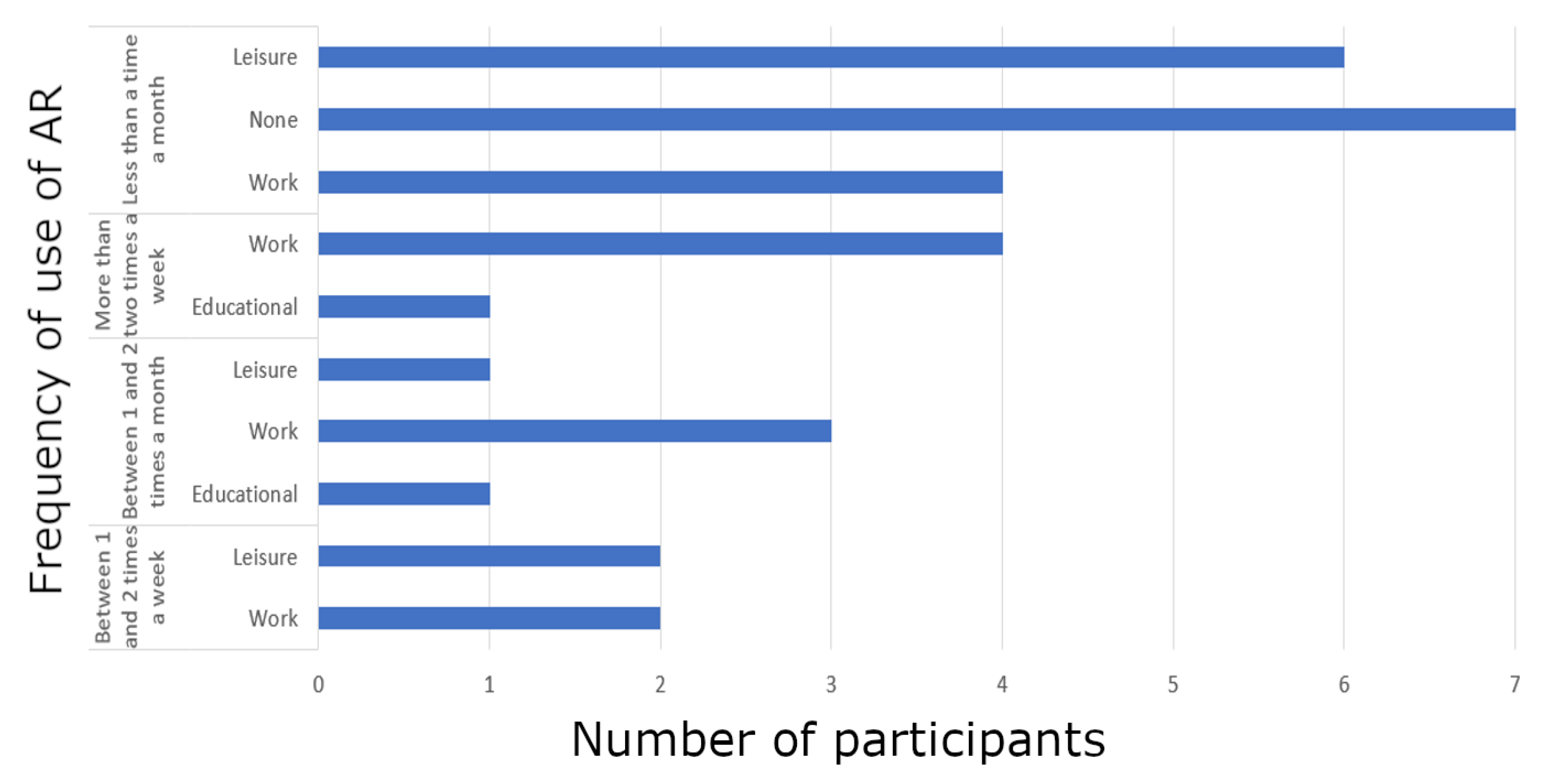
4.3.1. Subjects
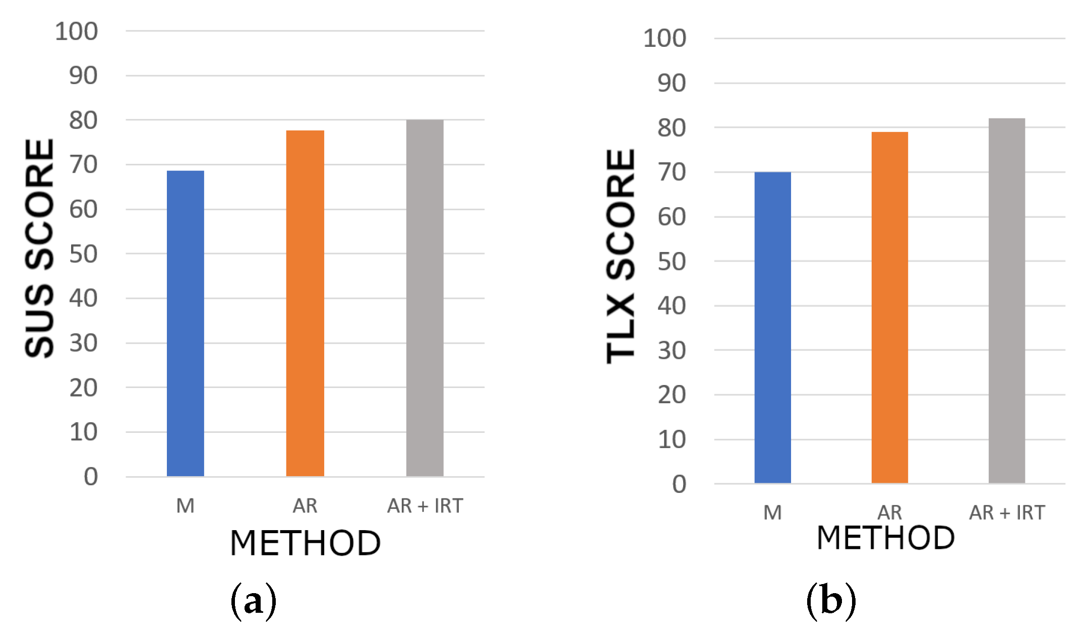
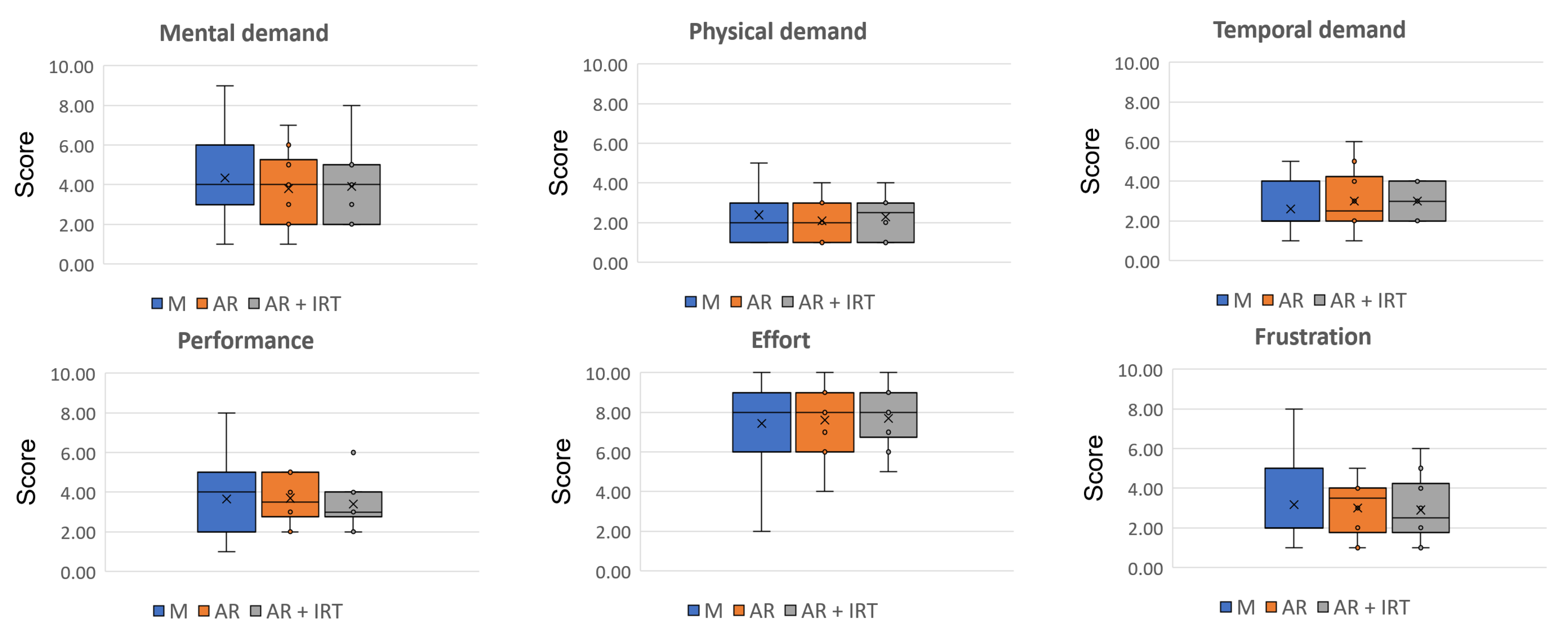
4.3.2. Results
5. Conclusions
Author Contributions
Funding
Institutional Review Board Statement
Informed Consent Statement
Data Availability Statement
Conflicts of Interest
Abbreviations
| AR | Augmented Reality |
| IRT | Infrared Radiation Thermography |
| 6DOF | 6 Degree of Freedom |
| LM | LINEMOD dataset |
| LM-O | LINEMOD-OCCLUDED dataset |
References
- Lamberti, F.; Manuri, F.; Sanna, A.; Paravati, G.; Pezzolla, P.; Montuschi, P. Challenges, opportunities, and future trends of emerging techniques for augmented reality-based maintenance. IEEE Trans. Emerg. Top. Comput. 2014, 2, 411–421. [Google Scholar] [CrossRef]
- Palmarini, R.; Erkoyuncu, J.A.; Roy, R.; Torabmostaedi, H. A systematic review of augmented reality applications in maintenance. Robot. Comput.-Integr. Manuf. 2018, 49, 215–228. [Google Scholar] [CrossRef]
- Lim, G.M.; Bae, D.M.; Kim, J.H. Fault diagnosis of rotating machine by thermography method on support vector machine. J. Mech. Sci. Technol. 2014, 28, 2947–2952. [Google Scholar] [CrossRef]
- Bagavathiappan, S.; Lahiri, B.; Saravanan, T.; Philip, J.; Jayakumar, T. Infrared thermography for condition monitoring—A review. Infrared Phys. Technol. 2013, 60, 35–55. [Google Scholar] [CrossRef]
- Jadin, M.S.; Taib, S. Recent progress in diagnosing the reliability of electrical equipment by using infrared thermography. Infrared Phys. Technol. 2012, 55, 236–245. [Google Scholar] [CrossRef]
- You, M.Y.; Liu, F.; Wang, W.; Meng, G. Statistically planned and individually improved predictive maintenance management for continuously monitored degrading systems. IEEE Trans. Reliab. 2010, 59, 744–753. [Google Scholar] [CrossRef]
- Zubizarreta, J.; Aguinaga, I.; Amundarain, A. A framework for augmented reality guidance in industry. Int. J. Adv. Manuf. Technol. 2019, 102, 4095–4108. [Google Scholar] [CrossRef]
- Maldague, X. Theory and practice of infrared technology for nondestructive testing. In Wiley Series in Microwave and Optical Engineering; Wiley: New York, NY, USA, 2001. [Google Scholar]
- Rytov, S.M. Theory of Electric Fluctuations and Thermal Radiation; Technical Report; Air force Cambridge Research Lab Hanscom: Arlington, TX, USA, 1959. [Google Scholar]
- Diakides, M.; Bronzino, J.D.; Peterson, D.R. Medical Infrared Imaging: Principles and Practices; CRC Press: Boca Raton, FL, USA, 2012. [Google Scholar]
- Balaras, C.A.; Argiriou, A. Infrared thermography for building diagnostics. Energy Build. 2002, 34, 171–183. [Google Scholar] [CrossRef]
- Fukuda, T.; Yokoi, K.; Yabuki, N.; Motamedi, A. An indoor thermal environment design system for renovation using augmented reality. J. Comput. Des. Eng. 2019, 6, 179–188. [Google Scholar] [CrossRef]
- Kurz, D. Thermal touch: Thermography-enabled everywhere touch interfaces for mobile augmented reality applications. In Proceedings of the 2014 IEEE International Symposium on Mixed and Augmented Reality (ISMAR), Munich, Germany, 10–12 September 2014; pp. 9–16. [Google Scholar]
- Cifuentes, I.J.; Dagnino, B.L.; Salisbury, M.C.; Perez, M.E.; Ortega, C.; Maldonado, D. Augmented reality and dynamic infrared thermography for perforator mapping in the anterolateral thigh. Arch. Plast. Surg. 2018, 45, 284. [Google Scholar] [CrossRef] [PubMed]
- Hinterstoisser, S.; Lepetit, V.; Ilic, S.; Holzer, S.; Bradski, G.; Konolige, K.; Navab, N. Model based training, detection and pose estimation of texture-less 3D objects in heavily cluttered scenes. In Proceedings of the Asian Conference on Computer Vision, Daejeon, Korea, 5–9 November 2012; pp. 548–562. [Google Scholar]
- Alexey, A. YOLOv4—Neural Networks for Object Detection (Windows and Linux Version of Darknet). 2020. Available online: https://github.com/AlexeyAB/darknet (accessed on 3 November 2020).
- Tjaden, H.; Schwanecke, U.; Schomer, E. Real-time monocular pose estimation of 3D objects using temporally consistent local color histograms. In Proceedings of the IEEE International Conference on Computer Vision, Venice, Italy, 22–29 October 2017; pp. 124–132. [Google Scholar]
- Denninger, M.; Sundermeyer, M.; Winkelbauer, D.; Zidan, Y.; Olefir, D.; Elbadrawy, M.; Lodhi, A.; Katam, H. BlenderProc. arXiv 2019, arXiv:1911.01911. [Google Scholar]
- Masood, T.; Egger, J. Augmented reality in support of Industry 4.0—Implementation challenges and success factors. Robot. Comput.-Integr. Manuf. 2019, 58, 181–195. [Google Scholar] [CrossRef]
- Fiorentino, M.; Uva, A.E.; Gattullo, M.; Debernardis, S.; Monno, G. Augmented reality on large screen for interactive maintenance instructions. Comput. Ind. 2014, 65, 270–278. [Google Scholar] [CrossRef]
- Ceruti, A.; Marzocca, P.; Liverani, A.; Bil, C. Maintenance in aeronautics in an Industry 4.0 context: The role of Augmented Reality and Additive Manufacturing. J. Comput. Des. Eng. 2019, 6, 516–526. [Google Scholar] [CrossRef]
- Webel, S.; Bockholt, U.; Engelke, T.; Gavish, N.; Olbrich, M.; Preusche, C. An augmented reality training platform for assembly and maintenance skills. Robot. Auton. Syst. 2013, 61, 398–403. [Google Scholar] [CrossRef]
- Castellanos, M.J.; Navarro-Newball, A.A. Prototyping an Augmented Reality Maintenance and Repairing System for a Deep Well Vertical Turbine Pump. In Proceedings of the 2019 International Conference on Electronics, Communications and Computers (CONIELECOMP), Cholula, Mexico, 27 February–1 March 2019; pp. 36–40. [Google Scholar]
- Alvarez, H.; Aguinaga, I.; Borro, D. Providing guidance for maintenance operations using automatic markerless augmented reality system. In Proceedings of the 2011 10th IEEE International Symposium on Mixed and Augmented Reality, Basel, Switzerland, 26–29 October 2011; pp. 181–190. [Google Scholar]
- Klein, G.; Murray, D. Parallel tracking and mapping for small AR workspaces. In Proceedings of the 2007 6th IEEE and ACM International Symposium on Mixed and Augmented Reality, Nara, Japan, 13–16 November 2007; pp. 225–234. [Google Scholar]
- Lowe, D.G. Distinctive image features from scale-invariant keypoints. Int. J. Comput. Vis. 2004, 60, 91–110. [Google Scholar] [CrossRef]
- Drost, B.; Ulrich, M.; Navab, N.; Ilic, S. Model globally, match locally: Efficient and robust 3D object recognition. In Proceedings of the 2010 IEEE Computer Society Conference on Computer Vision and Pattern Recognition, San Francisco, CA, USA, 13–18 June 2010; pp. 998–1005. [Google Scholar]
- Drummond, T.; Cipolla, R. Real-time visual tracking of complex structures. IEEE Trans. Pattern Anal. Mach. Intell. 2002, 24, 932–946. [Google Scholar] [CrossRef]
- Choi, C.; Christensen, H.I. Real-time 3D model-based tracking using edge and keypoint features for robotic manipulation. In Proceedings of the 2010 IEEE International Conference on Robotics and Automation, Anchorage, AK, USA, 3–8 May 2010; pp. 4048–4055. [Google Scholar]
- Prisacariu, V.A.; Reid, I.D. PWP3D: Real-time segmentation and tracking of 3D objects. Int. J. Comput. Vis. 2012, 98, 335–354. [Google Scholar] [CrossRef]
- Rad, M.; Lepetit, V. BB8: A scalable, accurate, robust to partial occlusion method for predicting the 3D poses of challenging objects without using depth. In Proceedings of the IEEE International Conference on Computer Vision, Venice, Italy, 22–29 October 2017; pp. 3828–3836. [Google Scholar]
- Kehl, W.; Manhardt, F.; Tombari, F.; Ilic, S.; Navab, N. Ssd-6D: Making RGB-based 3D detection and 6D pose estimation great again. In Proceedings of the IEEE International Conference on Computer Vision, Venice, Italy, 22–29 October 2017; pp. 1521–1529. [Google Scholar]
- Zakharov, S.; Shugurov, I.; Ilic, S. Dpod: 6D pose object detector and refiner. In Proceedings of the IEEE International Conference on Computer Vision, Seoul, Korea, 27 October–2 November 2019; pp. 1941–1950. [Google Scholar]
- Su, Y.; Rambach, J.; Minaskan, N.; Lesur, P.; Pagani, A.; Stricker, D. Deep Multi-state Object Pose Estimation for Augmented Reality Assembly. In Proceedings of the 2019 IEEE International Symposium on Mixed and Augmented Reality Adjunct (ISMAR-Adjunct), Beijing, China, 14–18 October 2019; pp. 222–227. [Google Scholar]
- Ivorra, E.; Ortega, M.; Catalán, J.; Ezquerro, S.; Lledó, L.; Garcia-Aracil, N.; Alcañiz, M. Intelligent Multimodal Framework for Human Assistive Robotics Based on Computer Vision Algorithms. Sensors 2018, 18, 2408. [Google Scholar] [CrossRef]
- Hodan, T.; Haluza, P.; Obdržálek, Š.; Matas, J.; Lourakis, M.; Zabulis, X. T-LESS: An RGB-D dataset for 6D pose estimation of texture-less objects. In Proceedings of the 2017 IEEE Winter Conference on Applications of Computer Vision (WACV), Santa Rosa, CA, USA, 24–31 March 2017; pp. 880–888. [Google Scholar]
- Du, B.; He, Y.; He, Y.; Zhang, C. Progress and trends in fault diagnosis for renewable and sustainable energy system based on infrared thermography: A review. Infrared Phys. Technol. 2020, 109, 103383. [Google Scholar] [CrossRef]
- Lopez-Perez, D.; Antonino-Daviu, J. Application of infrared thermography to failure detection in industrial induction motors: Case stories. IEEE Trans. Ind. Appl. 2017, 53, 1901–1908. [Google Scholar] [CrossRef]
- Hakimollahi, H.; Zamani, D.; Hosseini, S.H.; Rahimi, R.; Abbasi, M. Evaluation of thermography inspections effects on costs and power losses reduction in Alborz Province Power Distribution Co. In Proceedings of the 2016 21st Conference on Electrical Power Distribution Networks Conference (EPDC), Karaj, Iran, 26–27 April 2016; pp. 222–226. [Google Scholar]
- Leal-Meléndrez, J.A.; Altamirano-Robles, L.; Gonzalez, J.A. Occlusion handling in video-based augmented reality using the kinect sensor for indoor registration. In Iberoamerican Congress on Pattern Recognition; Springer: Berlin, Germany, 2013; pp. 447–454. [Google Scholar]
- Hinterstoisser, S.; Cagniart, C.; Ilic, S.; Sturm, P.; Navab, N.; Fua, P.; Lepetit, V. Gradient response maps for real-time detection of textureless objects. IEEE Trans. Pattern Anal. Mach. Intell. 2011, 34, 876–888. [Google Scholar] [CrossRef] [PubMed]
- Zhang, Z. Iterative point matching for registration of free-form curves and surfaces. Int. J. Comput. Vis. 1994, 13, 119–152. [Google Scholar] [CrossRef]
- Chen, S.; Hong, J.; Liu, X.; Li, J.; Zhang, T.; Wang, D.; Guan, Y. A Framework for 3D Object Detection and Pose Estimation in Unstructured Environment Using Single Shot Detector and Refined LineMOD Template Matching. In Proceedings of the 2019 24th IEEE International Conference on Emerging Technologies and Factory Automation (ETFA), Zaragoza, Spain, 10–13 September 2019; pp. 499–504. [Google Scholar]
- Liu, W.; Anguelov, D.; Erhan, D.; Szegedy, C.; Reed, S.; Fu, C.Y.; Berg, A.C. Ssd: Single shot multibox detector. In European Conference on Computer Vision; Springer: Berlin, Germany, 2016; pp. 21–37. [Google Scholar]
- Bochkovskiy, A.; Wang, C.Y.; Liao, H.Y.M. YOLOv4: Optimal Speed and Accuracy of Object Detection. arXiv 2020, arXiv:2004.10934. [Google Scholar]
- Lin, T.Y.; Maire, M.; Belongie, S.; Hays, J.; Perona, P.; Ramanan, D.; Dollár, P.; Zitnick, C.L. Microsoft coco: Common objects in context. In European Conference on Computer Vision; Springer: Berlin, Germany, 2014; pp. 740–755. [Google Scholar]
- Redmon, J.; Farhadi, A. Yolov3: An incremental improvement. arXiv 2018, arXiv:1804.02767. [Google Scholar]
- Lin, T.Y.; Goyal, P.; Girshick, R.; He, K.; Dollár, P. Focal loss for dense object detection. In Proceedings of the IEEE International Conference on Computer Vision, Venice, Italy, 22–29 October 2017; pp. 2980–2988. [Google Scholar]
- Ren, S.; He, K.; Girshick, R.; Sun, J. Faster r-cnn: Towards real-time object detection with region proposal networks. IEEE Trans. Pattern Anal. Mach. Intell. 2016, 39, 1137–1149. [Google Scholar] [CrossRef]
- Dwibedi, D.; Misra, I.; Hebert, M. Cut, Paste and Learn: Surprisingly Easy Synthesis for Instance Detection. In Proceedings of the 2017 IEEE International Conference on Computer Vision (ICCV), Venice, Italy, 22–29 October 2017; pp. 1310–1319. [Google Scholar]
- Tremblay, J.; Prakash, A.; Acuna, D.; Brophy, M.; Jampani, V.; Anil, C.; To, T.; Cameracci, E.; Boochoon, S.; Birchfield, S. Training deep networks with synthetic data: Bridging the reality gap by domain randomization. In Proceedings of the IEEE Conference on Computer Vision and Pattern Recognition Workshops, Salt Lake City, UT, USA, 18–22 June 2018; pp. 969–977. [Google Scholar]
- Hodaň, T.; Vineet, V.; Gal, R.; Shalev, E.; Hanzelka, J.; Connell, T.; Urbina, P.; Sinha, S.N.; Guenter, B. Photorealistic Image Synthesis for Object Instance Detection. In Proceedings of the 2019 IEEE International Conference on Image Processing (ICIP), Taipei, Taiwan, 22–25 September 2019; pp. 66–70. [Google Scholar]
- Dai, J.S. Euler–Rodrigues formula variations, quaternion conjugation and intrinsic connections. Mech. Mach. Theory 2015, 92, 144–152. [Google Scholar] [CrossRef]
- Brown, D.C. Decentering distortion of lenses. Photogramm. Eng. Remote. Sens. 1966, 32, 444–462. [Google Scholar]
- Zhang, Z. A flexible new technique for camera calibration. IEEE Trans. Pattern Anal. Mach. Intell. 2000, 22, 1330–1334. [Google Scholar] [CrossRef]
- Fischler, M.; Bolles, R. Random sample consensus: A paradigm for model fitting with applications to image analysis and automated cartography. Commun. ACM 1981, 24, 381–395. [Google Scholar] [CrossRef]
- Rangel, J.; Soldan, S.; Kroll, A. 3D thermal imaging: Fusion of thermography and depth cameras. In Proceedings of the International Conference on Quantitative InfraRed Thermography, Bordeaux, France, 7–11 July 2014; Volume 3. [Google Scholar]
- Vidas, S.; Lakemond, R.; Denman, S.; Fookes, C.; Sridharan, S.; Wark, T. A mask-based approach for the geometric calibration of thermal-infrared cameras. IEEE Trans. Instrum. Meas. 2012, 61, 1625–1635. [Google Scholar] [CrossRef]
- Brachmann, E.; Krull, A.; Michel, F.; Gumhold, S.; Shotton, J.; Rother, C. Learning 6D object pose estimation using 3D object coordinates. In European Conference on Computer Vision; Springer: Berlin, Germany, 2014; pp. 536–551. [Google Scholar]
- Brachmann, E.; Michel, F.; Krull, A.; Ying Yang, M.; Gumhold, S. Uncertainty-driven 6D pose estimation of objects and scenes from a single rgb image. In Proceedings of the IEEE Conference on Computer Vision and Pattern Recognition, Las Vegas, NV, USA, 27–30 June 2016; pp. 3364–3372. [Google Scholar]
- Song, C.; Song, J.; Huang, Q. Hybridpose: 6D object pose estimation under hybrid representations. In Proceedings of the IEEE/CVF Conference on Computer Vision and Pattern Recognition, Seattle, WA, USA, 13–19 June 2020; pp. 431–440. [Google Scholar]
- Aguilar, M.I.H.; Villegas, A.A.G. Análisis comparativo de la Escala de Usabilidad del Sistema (EUS) en dos versiones/Comparative analysis of the System Usability Scale (SUS) in two versions. RECI Rev. Iberoam. Las Cienc. Comput. Inform. 2016, 5, 44–58. [Google Scholar]
- Martinetti, A.; Rajabalinejad, M.; Van Dongen, L. Shaping the future maintenance operations: Reflections on the adoptions of Augmented Reality through problems and opportunities. Procedia CIRP 2017, 59, 14–17. [Google Scholar] [CrossRef]
- Glowacz, A. Fault diagnosis of electric impact drills using thermal imaging. Measurement 2021, 171, 108815. [Google Scholar] [CrossRef]


| Markerless | |||
| Model-based | |||
| Tracking by detection | |||
| Marker-based [20] | SLAM-based [25] | • Local appearance features [26] | |
| • Local 3D geometric descriptors [27] | 6DOF pose tracking [17,28,29,30] | ||
| • Template-based [15] | |||
| • Deep-learning methods [31,32,33,34] | |||
| Input Images Size | Batch Size | Subdivisions | Momentum | Initial Learning Rate | Decay | Max Batches |
|---|---|---|---|---|---|---|
| 416 × 416 | 64 | 8 | 0.949 | 0.0003 | 0.0005 | 40k |
| Dataset | mAP@.5 IOU | mAP@.75 IOU |
|---|---|---|
| LM | 99.01% | 94.24% |
| LM-O | 91.46% | 72.55% |
| Model | LM | LM-O | ||||||
|---|---|---|---|---|---|---|---|---|
| LINEYOLO | LINEMOD | LINEYOLO | LINEMOD | |||||
| ADD | Proj.2D | ADD | Proj.2D | ADD | Proj.2D | ADD | Proj.2D | |
| Ape | 97.97% | 98.62% | 94.17% | 94.41% | 63.24% | 68.11% | 58.80% | 62.73% |
| Bench Vise | 99.01% | 98.84% | 97.94% | 97.04% | × | × | × | × |
| Bowl | 96.48% | 93.34% | 95.13% | 94.32% | × | × | × | × |
| Cam | 90.00% | 89.67% | 89.34% | 89.34% | × | × | × | × |
| Can | 92.05% | 95.31% | 89.54% | 93.06% | × | × | × | × |
| Cat | 99.15% | 99.32% | 96.52% | 96.52% | 63.19% | 64.66% | 49.18% | 50.90% |
| Cup | 95.72% | 79.75% | 91.12% | 75.32% | 17.42% | 17.69% | 12.58% | 12.58% |
| Driller | 88.55% | 86.36% | 81.73% | 78.11% | 36.88% | 34.77% | 27.81% | 26.32% |
| Duck | 96.73% | 98.96% | 95.77% | 96.65% | 60.28% | 69.29% | 54.08% | 60.38% |
| Box | 98.48% | 98.16% | 98.96% | 98.80% | 29.57% | 25.72% | 18.30% | 17.14% |
| Glue | 91.55% | 88.85% | 56.39% | 54.67% | 33.33% | 27.92% | 8.67% | 8.30% |
| Hole Punch | 97.00% | 97.49% | 74.13% | 74.13% | 90.05% | 90.68% | 59.06% | 59.19% |
| Iron | 96.78% | 96.70% | 92.79% | 92.62% | × | × | × | × |
| Lamp | 92.99% | 91.76% | 84.59% | 83.86% | × | × | × | × |
| Phone | 91.15% | 90.82% | 67.09% | 66.93% | × | × | × | × |
| Average | 94.90% | 93.59% | 87.01% | 85.71% | 49.24% | 49.85% | 36.06% | 37.19% |
| PHASE | PARTS | TIME (s) | |
|---|---|---|---|
| Initial detector and pose estimation | Option 1: | LINEMOD | 0.069 |
| Option 2: | YOLOV4 | 0.036 | |
| LINEYOLO | LINEMOD | 0.035 | |
| Parallel ICP | 0.051 | ||
| 6DOF pose tracking | Tjaden et al. method [17] | 0.023 | |
| IRT Fusion | IRT to RGB-D Registration | 0.012 | |
| Metric | Diagnosis Task | Repair Task | |||||
|---|---|---|---|---|---|---|---|
| M | AR | AR + IRT | M | AR | AR + IRT | ||
| Time (Minutes) | Mean value | 6.74 | 6.00 | 5.60 | 5.01 | 4.07 | 3.91 |
| Standard deviation | 5.45 | 3.21 | 2.35 | 2.58 | 1.34 | 2.00 | |
| Reduction (%) | −10.98 | −16.88 | −18.81 | −21.84 | |||
| Errors (Quantity) | Mean value | 3.60 | 1.33 | 1.00 | 3.1 | 1.4 | 0.8 |
| Standard deviation | 2.27 | ||||||
| Reduction (%) | −62.96 | −72.22 | −54.84 | −74.19 | |||
Publisher’s Note: MDPI stays neutral with regard to jurisdictional claims in published maps and institutional affiliations. |
© 2021 by the authors. Licensee MDPI, Basel, Switzerland. This article is an open access article distributed under the terms and conditions of the Creative Commons Attribution (CC BY) license (http://creativecommons.org/licenses/by/4.0/).
Share and Cite
Ortega, M.; Ivorra, E.; Juan, A.; Venegas, P.; Martínez, J.; Alcañiz, M. MANTRA: An Effective System Based on Augmented Reality and Infrared Thermography for Industrial Maintenance. Appl. Sci. 2021, 11, 385. https://doi.org/10.3390/app11010385
Ortega M, Ivorra E, Juan A, Venegas P, Martínez J, Alcañiz M. MANTRA: An Effective System Based on Augmented Reality and Infrared Thermography for Industrial Maintenance. Applied Sciences. 2021; 11(1):385. https://doi.org/10.3390/app11010385
Chicago/Turabian StyleOrtega, Mario, Eugenio Ivorra, Alejandro Juan, Pablo Venegas, Jorge Martínez, and Mariano Alcañiz. 2021. "MANTRA: An Effective System Based on Augmented Reality and Infrared Thermography for Industrial Maintenance" Applied Sciences 11, no. 1: 385. https://doi.org/10.3390/app11010385
APA StyleOrtega, M., Ivorra, E., Juan, A., Venegas, P., Martínez, J., & Alcañiz, M. (2021). MANTRA: An Effective System Based on Augmented Reality and Infrared Thermography for Industrial Maintenance. Applied Sciences, 11(1), 385. https://doi.org/10.3390/app11010385