A Theoretical Model with Which to Safely Optimize the Configuration of Hydraulic Suspension of Modular Trailers in Special Road Transport

 ,
,  ,
, 
 and
and 
Abstract
1. Introduction
2. Materials and Methods
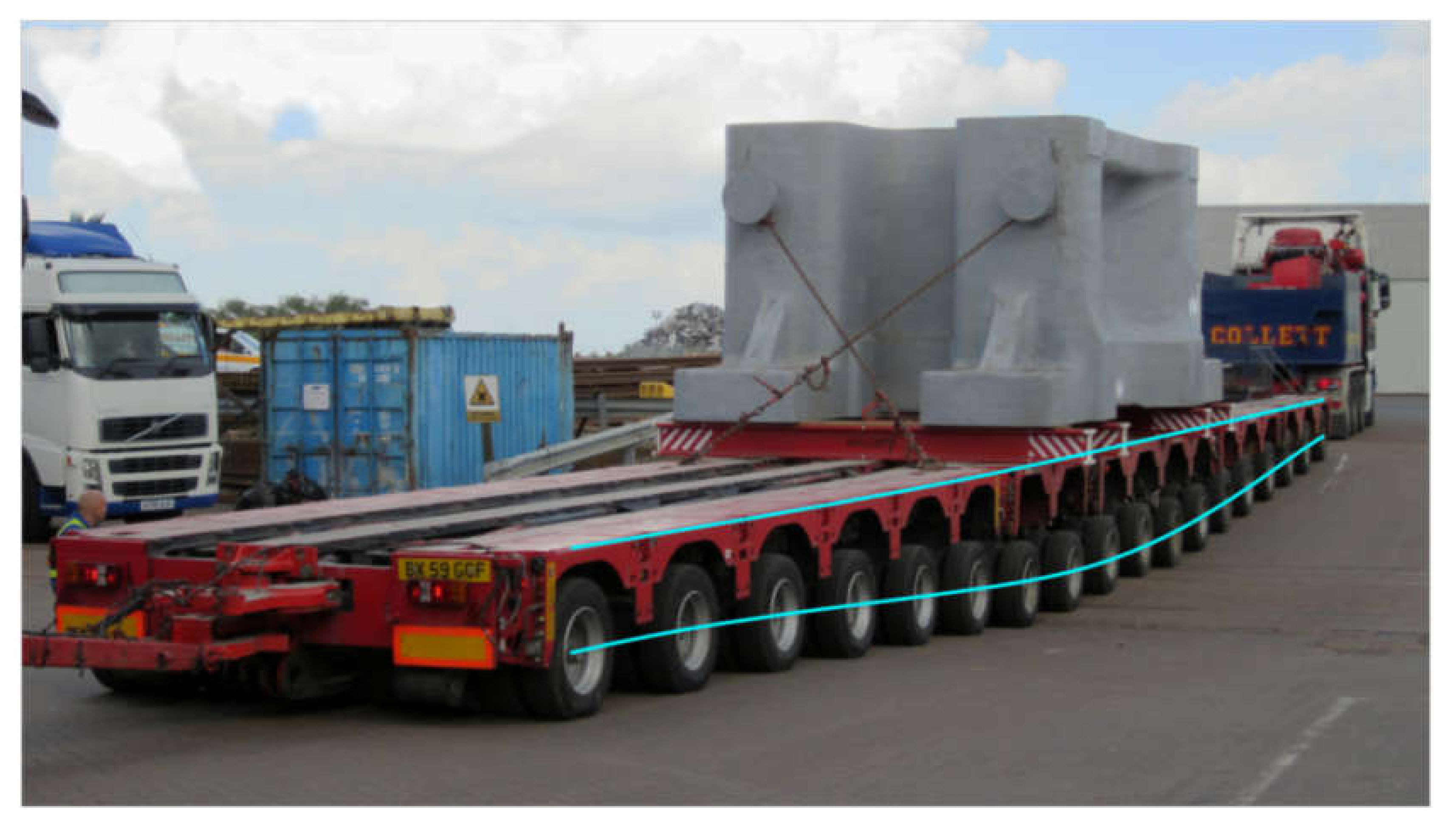
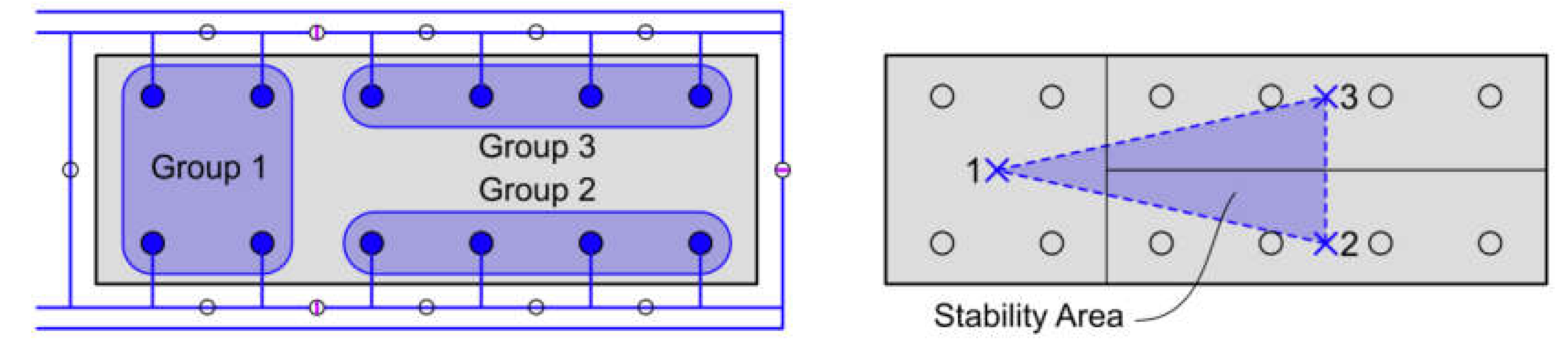
2.1. Modular Trailers
2.2. Stability Area
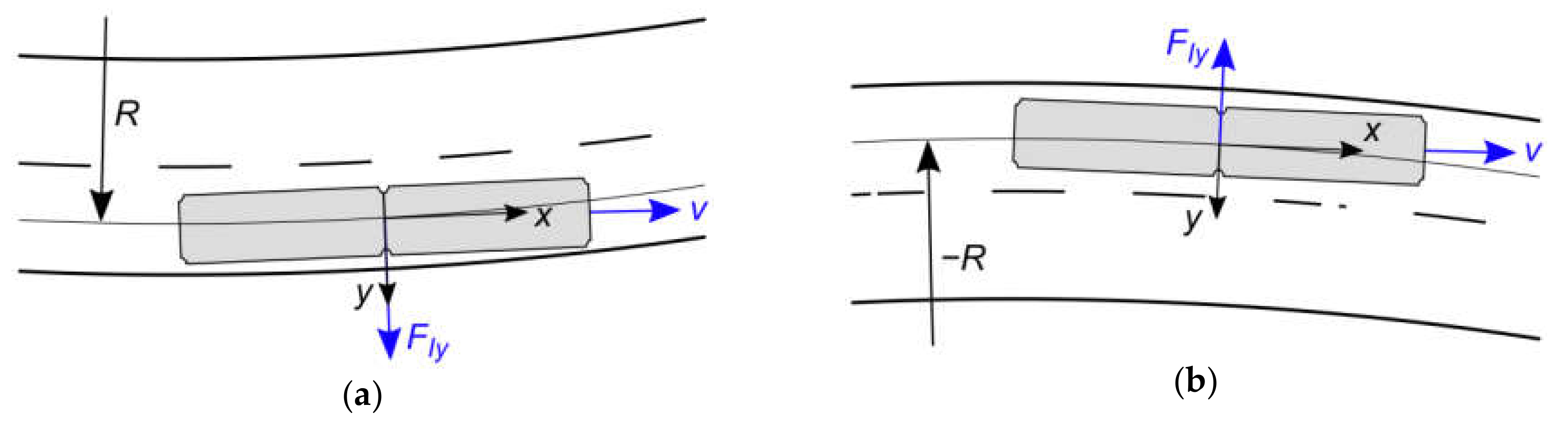
2.3. Forces Acting upon the Transportation Model
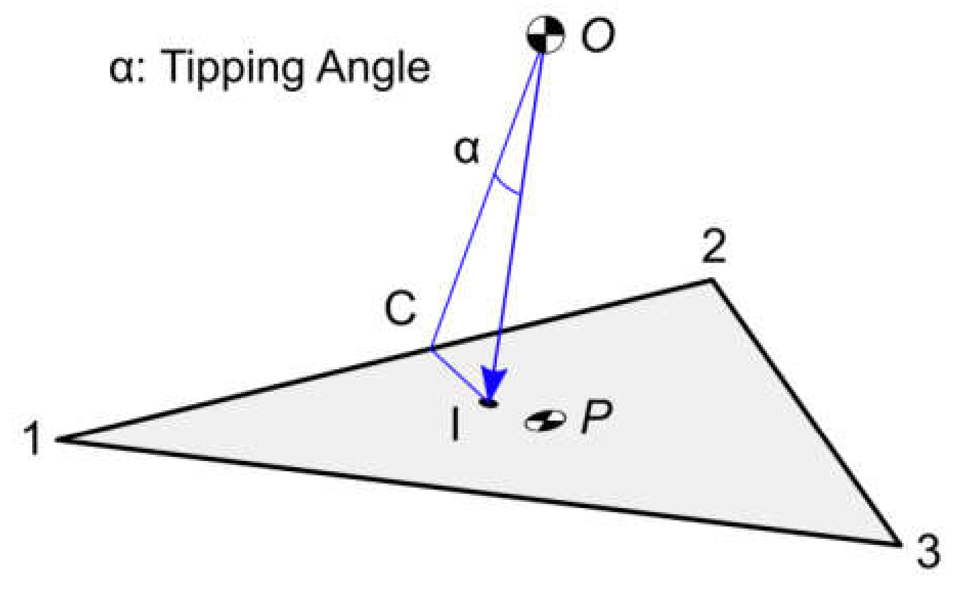
2.4. Stability Calculation
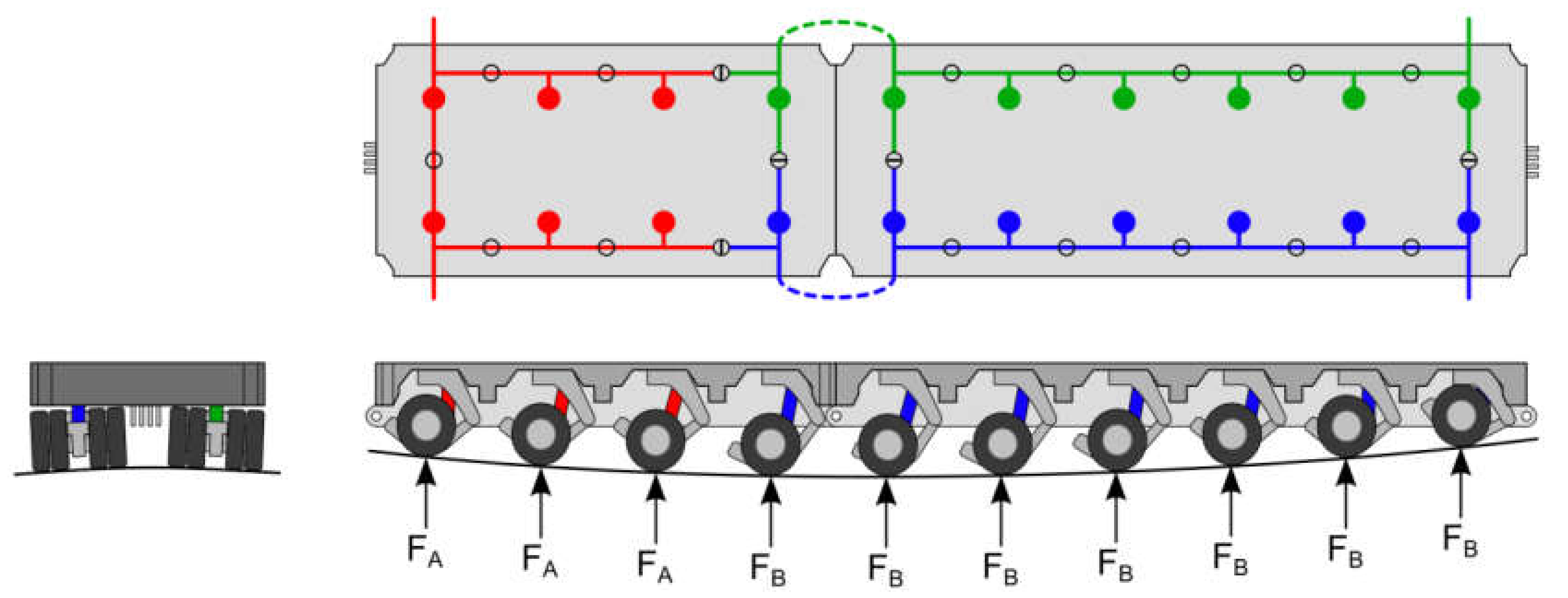
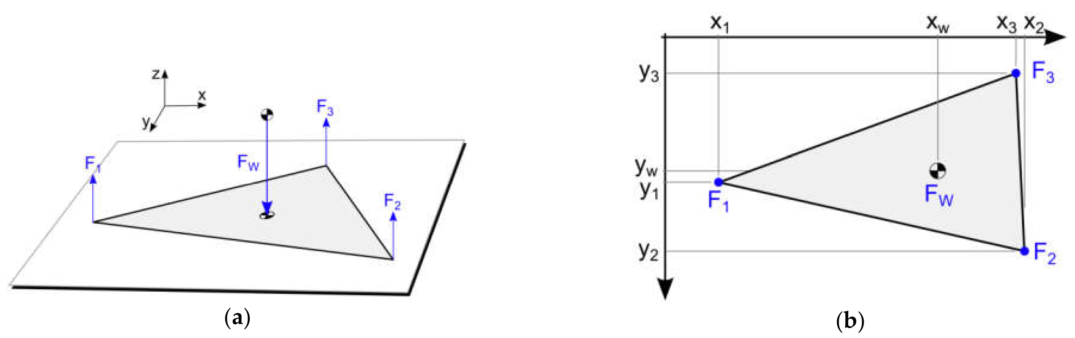
2.5. Reactions of the Suspension Groups
- Load (W) and reactions (F1, F2, and F3) are perpendicular to the stability plane.
- There are no forces in X or Y and/or moment in Z. Thus, the equilibrium equations are three in number.
- The system affects quasi-static loading. That is, it is assumed that the time and mass do not influence the load.
- The ground is assumed to be a completely rigid plane.
3. Results and Discussion
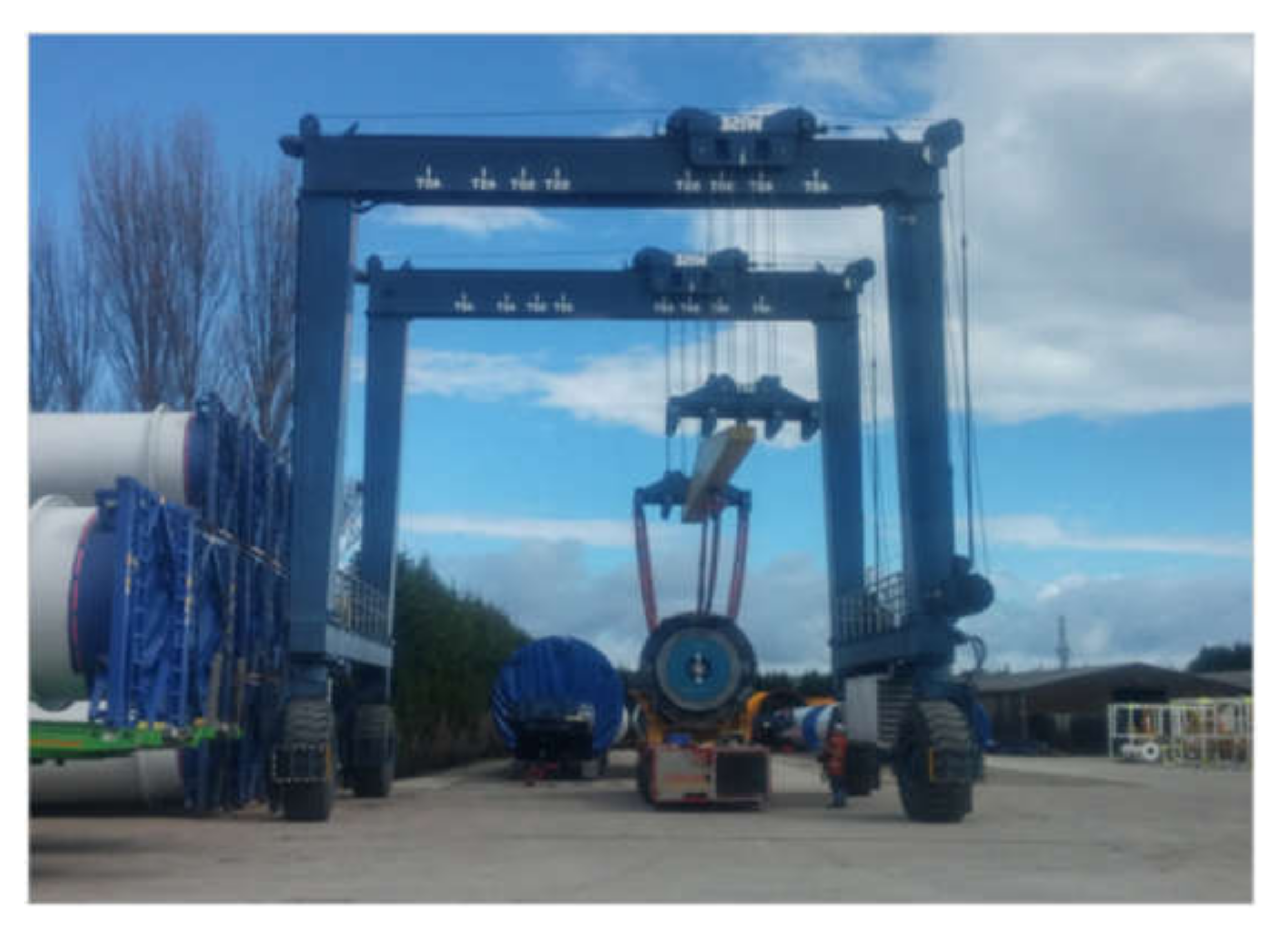
3.1. Experimental Validation of the Proposed Model
- Trailer: SPMT 6-axle: weight 23.5 and maximum capacity 216.3 Tn.
- The oil pressure is supplied to the hydraulic cylinders at the axles by a Power Unit (PPU).
- Even surface: camber and slope equal zero.
- Weight: 42,500 kg.
- Dimensions: 5133 × 2650 × 2975 mm.
- CoG position: 97.5 × 0 × −180 mm.
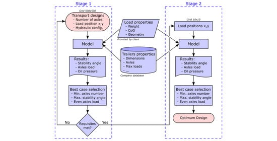
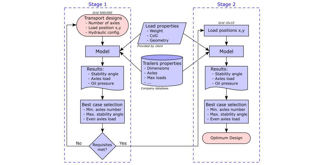
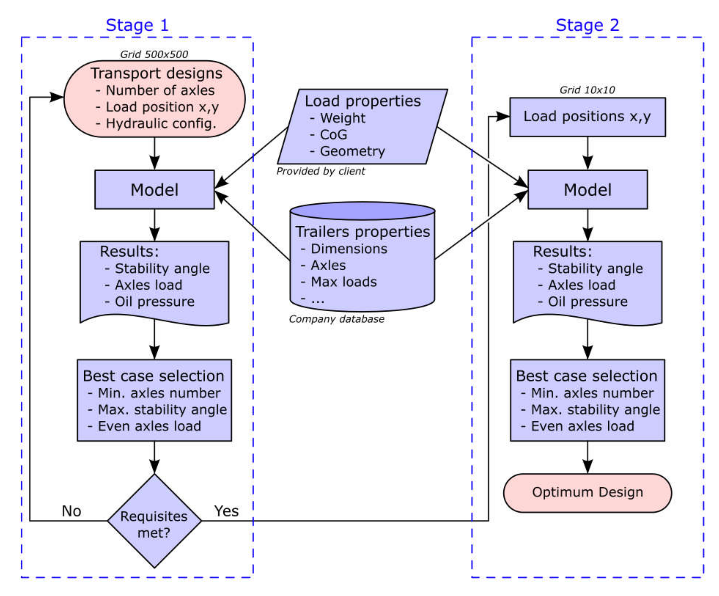
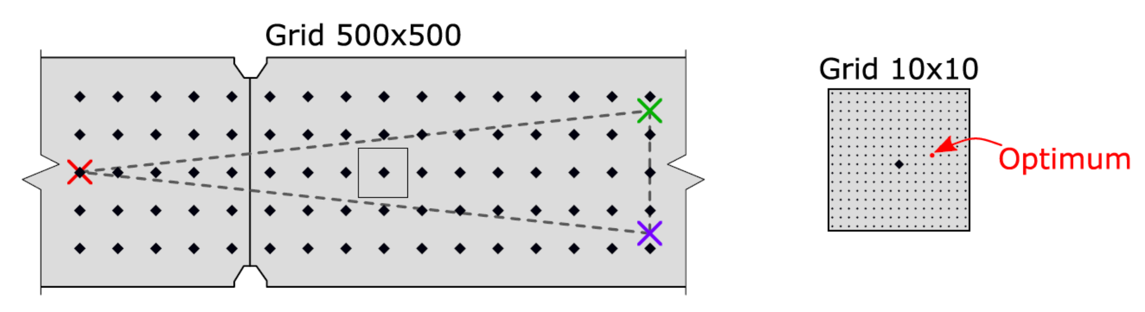
3.2. Optimization Process Proposed
4. Conclusions
Author Contributions
Funding
Institutional Review Board Statement
Informed Consent Statement
Data Availability Statement
Acknowledgments
Conflicts of Interest
References
- Gong, I.; Lee, K.; Kim, J.; Min, Y.; Shin, K. Optimizing Vehicle Routing for Simultaneous Delivery and Pick-Up Considering Reusable Transporting Containers: Case of Convenience Stores. Appl. Sci. 2020, 10, 4162. [Google Scholar] [CrossRef]
- Conesa, J.; Cavas-Martínez, F.; Fernández-Pacheco, D.G. An agent-based paradigm for detecting and acting on vehicles driving in the opposite direction on highways. Expert Syst. Appl. 2013, 40, 5113–5124. [Google Scholar] [CrossRef]
- Water Preferred Policy: Guidelines for the Movement of Abnormal Indivisible Loads; UK Highways Agency: Birmingham, UK, 2012.
- Taylor, N.B. The Impact of Abnormal Loads on Road Traffic Congestion; Transport Research Laboratory: Berkshire, UK, 2005. [Google Scholar]
- El-Gindy, M.; Kenis, W. Influence of a Trailer’s Axle Arrangement and Load on the Stability and Control of a Tractor Tractor-Semitrailer; Federal Highway Administration: Washington, DC, USA, 1998; p. 178.
- Lisowski, F.; Lisowski, E. Testing and Fatigue Life Assessment of Timber Truck Stanchions. Appl. Sci. 2020, 10, 6134. [Google Scholar] [CrossRef]
- Kim, J. Truck Platoon Control Considering Heterogeneous Vehicles. Appl. Sci. 2020, 10, 5067. [Google Scholar] [CrossRef]
- Zhao, L.; Zhang, Y.; Yu, Y.; Zhou, C.; Li, X.; Li, H. Truck Handling Stability Simulation and Comparison of Taper-Leaf and Multi-Leaf Spring Suspensions with the Same Vertical Stiffness. Appl. Sci. 2020, 10, 1293. [Google Scholar] [CrossRef]
- Ervin, R.D.; Nisonger, R.L.; Mallikarjunarao, C.; Gillespie, T.D. The Yaw Stability of Tractor-Semitrailers during Cornering; Technical Report for Transportation Research Institute: Ann Arbor, MI, USA, 1979. [Google Scholar]
- Chen, Y.; Huang, S.; Davis, L.; Du, H.; Shi, Q.; He, J.; Wang, Q.; Hu, W. Optimization of Geometric Parameters of Longitudinal-Connected Air Suspension Based on a Double-Loop Multi-Objective Particle Swarm Optimization Algorithm. Appl. Sci. 2018, 8, 1454. [Google Scholar] [CrossRef]
- Guowei, D.; Wenhao, Y.; Zhongxing, L.; Khajepour, A.; Senqi, T. Sliding Mode Control of Laterally Interconnected Air Suspensions. Appl. Sci. 2020, 10, 4320. [Google Scholar] [CrossRef]
- Martínez, F.C.; Fernandez-Pacheco, D.G. Simulación virtual: Una tecnología para el impulso de la innovación y la competitividad en la industria. DYNA Ing. Ind. 2019, 94, 118–119. [Google Scholar]
- García, L.O.; Wilson, F.R.; Innes, J.D. Heavy truck dynamic rollover: Effect of load distribution, cargo type, and road design characteristics. Transp. Res. Rec. J. Transp. Res. Board 2003, 1851, 25–31. [Google Scholar] [CrossRef]
- Ervin, R.D.; Yoram, G. The Influence of Weights and Dimensions on the Stability and Control of Heavy Duty Trucks in Canada; Transportation Association of Canada: Ottawa, ON, Canada, 1986; Volume I, p. 132. [Google Scholar]
- Gertsch, J.; Eichelhard, O. Simulation of Dynamic Rollover Threshold for Heavy Trucks; SAE International: Warrendale, PA, USA, 2003. [Google Scholar]
- Bernard, J.; Shannan, J.; Vanderploeg, M. Vehicle Rollover on Smooth Surfaces; SAE International: Warrendale, PA, USA, 1989. [Google Scholar]
- Winkler, C.B.; Blower, D.; Ervin, R.; Chalasani, R.M. Rollover of Heavy Commercial Vehicle; University of Michigan Transportation Research Institute: Ann Arbor, MI, USA, 2000. [Google Scholar]
- BS EN 12195-1:2010. Load Restraining on Road Vehicles—Safety. Part 1: Calculation of Securing Forces; BSI: London, UK, 2013. [Google Scholar]
- Zhang, Q.; Su, C.; Zhou, Y.; Zhang, C.; Ding, J.; Wang, Y. Numerical Investigation on Handling Stability of a Heavy Tractor Semi-Trailer under Crosswind. Appl. Sci. 2020, 10, 3672. [Google Scholar] [CrossRef]
- Cooper, K.R.; Watkins, S. The Unsteady Wind Environment of Road Vehicles, Part One: A Review of the on-Road Turbulent Wind Environment; SAE International: Warrendale, PA, USA, 2007; pp. 1259–1276. [Google Scholar]
- Cai, C.S.; Chen, S.R. Framework of vehicle–bridge–wind dynamic analysis. J. Wind Eng. Ind. Aerodyn. 2004, 92, 579–607. [Google Scholar] [CrossRef]
- Hammache, M.; Browand, F. On the Aerodynamics of Tractor-Trailers. In The Aerodynamics of Heavy Vehicles: Trucks, Buses, and Trains; McCallen, R., Browand, F., Ross, J., Eds.; Springer: Berlin/Heidelberg, Germany, 2004; Volume 19, pp. 185–205. ISBN 978-3-642-53586-4. [Google Scholar]
- Mccallen, R.; Flowers, D.; Dunn, T.; Owens, J.; Browand, F.; Hammache, M.; Leonard, A.; Brady, M.; Salari, K.; Rutledge, W.; et al. Aerodynamic Drag of Heavy Vehicles (Class 7–8): Simulation and Benchmarking; SAE International: Warrendale, PA, USA, 2000. [Google Scholar]
- Bettle, J.; Holloway, A.G.L.; Venart, J.E.S. A Computational Study of the Aerodynamic Forces Acting on a Tractor-Trailer Vehicle on a Bridge in Cross-Wind. J. Wind Eng. Ind. Aerodyn. 2003, 91, 573–592. [Google Scholar] [CrossRef]
- Baker, C.J. The effects of high winds on vehicle behaviour. In Proceedings of the International Symposium on Advances in Bridge Aerodynamics, Copenhagen, Denmark, 10–13 May 1998; pp. 267–282. [Google Scholar]
- King, J.P.C.; Mikitiuk, M.J.; Davenport, A.G.; Isyumov, N. A Study of Wind Effects for the Northumberland Straits Crossing; Boundary Layer Wind Tunnel Laboratory, University of Western Ontario: London, ON, Canada, 1994. [Google Scholar]
- Scheuerle. Operating Instructions: Combi Modular Transport System. Available online: https://www.scheuerle.com/products/self-propelled-transporters/intercombi.html (accessed on 28 December 2020).
- Collett & Sons Ltd. Available online: https://www.collett.co.uk/ (accessed on 28 December 2020).
- Van Daal, M.J. The Art of the Heavy Transport; The Works international: London, UK, 2009. [Google Scholar]
- Corral Bobadilla, M.; Lostado Lorza, R.; Somovilla Gómez, F.; Escribano García, R. Adsorptive of Nickel in Wastewater by Olive Stone Waste: Optimization through Multi-Response Surface Methodology Using Desirability Functions. Water 2020, 12, 1320. [Google Scholar] [CrossRef]
- Somovilla-Gómez, F.; Lostado-Lorza, R.; Corral-Bobadilla, M.; Escribano-García, R. Improvement in determining the risk of damage to the human lumbar functional spinal unit considering age, height, weight and sex using a combination of FEM and RSM. Biomech. Model. Mechanobiol. 2020, 19, 351–387. [Google Scholar] [CrossRef] [PubMed]
- Íñiguez-Macedo, S.; Lostado-Lorza, R.; Escribano-García, R.; Martínez-Calvo, M.Á. Finite Element Model Updating Combined with Multi-Response Optimization for Hyper-Elastic Materials Characterization. Materials 2019, 12, 1019. [Google Scholar] [CrossRef] [PubMed]
- Ruiz, L.; Torres, M.; Gómez, A.; Díaz, S.; González, J.M.; Cavas, F. Detection and Classification of Aircraft Fixation Elements during Manufacturing Processes Using a Convolutional Neural Network. Appl. Sci. 2020, 10, 6856. [Google Scholar] [CrossRef]
- Fisher, R.A. The Design of Experiments; Hafner Press: New York, NY, USA, 1974; ISBN 0-02-844690-9. [Google Scholar]
- Lendrem, D.; Owen, M.; Godbert, S. DOE (design of experiments) in development chemistry: Potential obstacles. Org. Process Res. Dev. 2001, 5, 324–327. [Google Scholar] [CrossRef]
- Weissman, S.A.; Anderson, N.G. Design of experiments (DoE) and process optimization. A review of recent publications. Org. Process Res. Dev. 2015, 19, 1605–1633. [Google Scholar] [CrossRef]
- R Core Team. R Core Team. R: A Language and Environment for Statistical Computing. Available online: https://www.r-project.org/ (accessed on 28 December 2020).
- InterCombi. Available online: https://www.scheuerle.com/products/self-propelled-transporters/intercombi.html (accessed on 28 December 2020).


| Inputs | Symbol | Unit | Levels | ||
|---|---|---|---|---|---|
| −1 | 0 | +1 | |||
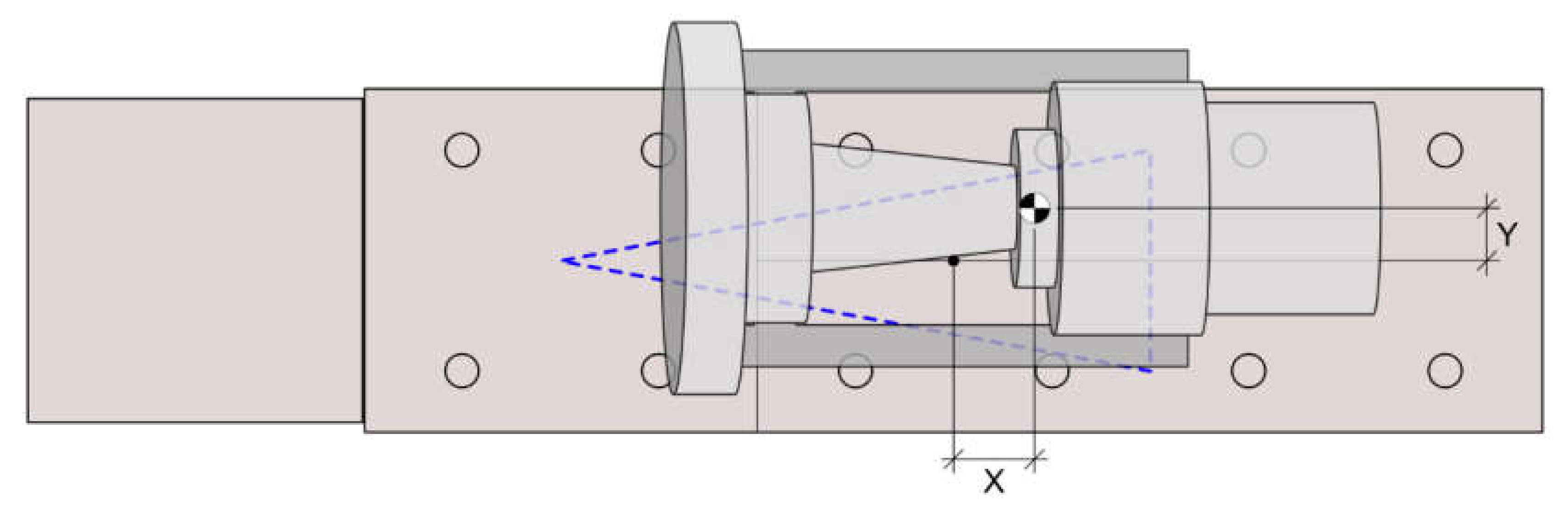
| Longitudinal location of the load | X | mm | 0 | 675 | 1350 |
| Transversal location of the load | Y | mm | 0 | 175 | 350 |
| X | Y | Pressures [bar] | ||||
|---|---|---|---|---|---|---|
| A | B | C | D | |||
| 1 | 0 | 0 | 59 | 61 | 77 | 75 |
| 2 | 0 | 0 | 55 | 62 | 80 | 79 |
| 3 | 0 | 0 | 60 | 61 | 75 | 72 |
| 4 | 0 | 0 | 64 | 56 | 90 | 92 |
| 5 | 0 | 0 | 58 | 63 | 78 | 74 |
| 6 | 0 | 335 | 24 | 97 | 80 | 80 |
| 7 | 0 | 435 | 13 | 108 | 81 | 85 |
| 8 | 675 | 0 | 66 | 75 | 58 | 58 |
| 9 | 675 | 335 | 38 | 103 | 58 | 59 |
| 10 | 675 | 435 | 27 | 117 | 58 | 58 |
| 11 | 1350 | 0 | 79 | 85 | 39 | 40 |
| 12 | 1350 | 335 | 47 | 120 | 39 | 38 |
| 13 | 1350 | 435 | 38 | 127 | 38 | 38 |
| Case | Range | Mean [μ] | SD [s] |
|---|---|---|---|
| Pressure A | 9 bar | 59.2 bar | 2.9 bar |
| Pressure B | 7 bar | 60.6 bar | 2.4 bar |
| Pressure C | 15 bar | 80.0 bar | 5.3 bar |
| Pressure D | 20 bar | 78.4 bar | 7.2 bar |
| Average values | 69.55 bar | 4.45 bar |
| Case | Pressures | ||||
|---|---|---|---|---|---|
| A [bar] | B [bar] | C [bar] | D [bar] | MAPE [%] | |
| 1–5 | 59.0 | 58.0 | 84.4 | 84.4 | 4.4 |
| 6 | 28.0 | 89.3 | 84.4 | 84.4 | 8.8 |
| 7 | 18.3 | 98.7 | 84.4 | 84.4 | 13.6 |
| 8 | 69.8 | 68.9 | 62.6 | 62.6 | 7.4 |
| 9 | 38.6 | 100.2 | 62.6 | 62.6 | 4.6 |
| 10 | 29.2 | 109.6 | 62.6 | 62.6 | 7.6 |
| 11 | 80.7 | 79.8 | 40.9 | 40.9 | 3.8 |
| 12 | 49.4 | 111.1 | 40.9 | 40.9 | 6.2 |
| 13 | 40.1 | 120.4 | 40.9 | 40.9 | 6.4 |
| Average: | 7.0% | ||||
| Characteristics | Value |
|---|---|
| Load | Cylindrical tank |
| Dimensions | 19.5 × 3.2 × 2.5 m |
| Load weight | 108,500 kg |
| Trailer weight | 33,000 kg |
| Initial CoG coordinates | 0.0 × 0.2 × 2.1 m |
| Optimum CoG coordinates | 0.3 × 0.0 × 2.1 m |
| Number of trailers | 2 |
| Number of axles | 10 (4 + 6) |
| Tipping angle (on even road) | 7.2° |
| Maximum axle load | 21,600 kg |
| Oil pressures | 8.1 × 8.1 × 5.9 bar |
| Hydraulic configuration | 6, 7, 7 |
Publisher’s Note: MDPI stays neutral with regard to jurisdictional claims in published maps and institutional affiliations. |
© 2020 by the authors. Licensee MDPI, Basel, Switzerland. This article is an open access article distributed under the terms and conditions of the Creative Commons Attribution (CC BY) license (http://creativecommons.org/licenses/by/4.0/).
Share and Cite
Escribano-García, R.; Corral-Bobadilla, M.; Somovilla-Gómez, F.; Lostado-Lorza, R.; Ahmed, A. A Theoretical Model with Which to Safely Optimize the Configuration of Hydraulic Suspension of Modular Trailers in Special Road Transport. Appl. Sci. 2021, 11, 305. https://doi.org/10.3390/app11010305
Escribano-García R, Corral-Bobadilla M, Somovilla-Gómez F, Lostado-Lorza R, Ahmed A. A Theoretical Model with Which to Safely Optimize the Configuration of Hydraulic Suspension of Modular Trailers in Special Road Transport. Applied Sciences. 2021; 11(1):305. https://doi.org/10.3390/app11010305
Chicago/Turabian StyleEscribano-García, Rubén, Marina Corral-Bobadilla, Fátima Somovilla-Gómez, Rubén Lostado-Lorza, and Ash Ahmed. 2021. "A Theoretical Model with Which to Safely Optimize the Configuration of Hydraulic Suspension of Modular Trailers in Special Road Transport" Applied Sciences 11, no. 1: 305. https://doi.org/10.3390/app11010305
APA StyleEscribano-García, R., Corral-Bobadilla, M., Somovilla-Gómez, F., Lostado-Lorza, R., & Ahmed, A. (2021). A Theoretical Model with Which to Safely Optimize the Configuration of Hydraulic Suspension of Modular Trailers in Special Road Transport. Applied Sciences, 11(1), 305. https://doi.org/10.3390/app11010305