Article

Traffic Simulation of Future Intelligent Vehicles in Duisburg City Inner Ring

Department of Mechatronics, University of Duisburg-Essen, 47057 Duisburg, Germany
*
Author to whom correspondence should be addressed.
Appl. Sci. 2021, 11(1), 29; https://doi.org/10.3390/app11010029
Submission received: 9 December 2020 / Revised: 18 December 2020 / Accepted: 21 December 2020 / Published: 23 December 2020

Abstract

:

Featured Application

This article can be applied to the simulations of vehicles with different degrees of automation in different city scenarios.

Abstract

Intelligent vehicles gradually enter the vehicular fleet with advanced driver-assistance technologies. Their impact on traffic should, therefore, be considered by transportation decision-makers. This paper examines the effect of vehicles with different levels of automation on traffic flow, such as non-assisted vehicles, vehicles with driver assistance systems, and fully autonomous vehicles. The accuracy of the examined traffic scenario is also an important factor in microscopic traffic simulation. In this paper, the central part of the city of Duisburg, Duisburg’s inner ring, is chosen for the traffic scenario. Through the cooperation with local government, official data of Origin/Destination matrices, induction loops, and traffic light plans are provided for this work. Thus, traffic demand from Origin/Destination matrices and induction loops are generated and compared, respectively. Finally, vehicles with different levels of automation are simulated in the Duisburg inner ring scenario.

1. Introduction

As the urban population grows continuously, traffic congestion, traffic accidents, and other negative impacts of the cities are becoming worse. The United Nations predict that, by 2050, the proportion of the global urban population will increase from 55 to 68% in 2018 [1]. The development of urbanization may increase residents’ demand for urban mobility, and emerging technologies including intelligent vehicles may make transportation modes more complicated but have the potential to address some of the problems mentioned. Worldwide, about 1.2 million people die from vehicle-related traffic accidents each year [2]; the resulting medical expenses, legal expenses, property losses, insurance costs, and loss of quality of life exceed 1 trillion US dollars [3]. The majority of traffic accidents can be attributed to human error, such as driving under external influences, drowsiness, or distraction. Automated vehicle systems support or replace human drivers with sensors such as cameras and radars. These devices that cannot be drunk, do not experience burnout, and cannot be distracted, and thus may reduce or even eliminate driver-related errors. Intelligent vehicles may have great significance for the development of public health. In addition to reducing traffic accident deaths, autonomous driving systems can improve people’s quality of life [2,4]. For energy consumption, partially automated vehicles might reduce greenhouse gas emissions and energy use by nearly half [5].
Before the realization of fully autonomous vehicles, the development of autonomous driving still faces many challenges [6]. However, a large number of simulation experiments and field trials are helping to promote the development of autonomous driving technology. As of August 2019, as many as 90 cities around the world have implemented pilot projects for autonomous vehicles [7]. So far, investment in the development of autonomous driving technology has reached more than 80 billion US dollars and is expected to show an upward trend [8]. Although some people expect the popularizing of fully autonomous vehicles by 2050 [9], the process of realization is still gradual, from few to many, from simple to complex. In the early stages of adopting autonomous vehicles, ordinary people cannot afford autonomous vehicles [4]. Although prices may decline in the foreseeable future, the cost of autonomous vehicles is expected to be higher than that of non-autonomous vehicles [10]. This has been reflected in the addition of existing vehicles and the addition of certain automatic functions, such as adaptive cruise control, night vision, and pedestrian detection, making vehicles equipped with these systems more expensive than ordinary vehicles. In addition to price factors, many drivers have doubts about the safety of autonomous vehicles. Urban residents and car users of different counties, ages, genders educational backgrounds, and income levels have different views on the current and future safety of autonomous vehicles [11]. Due to the considerations of price and safety, road vehicles will gradually shift from low level to high-level degrees of automation. The choice of different types of vehicle owners and the transformation of urban alternative transportation modes (such as car-sharing and self-driving taxis) will result in a long hybrid period of vehicles of various automation levels. From the perspective of travel demand, almost 85% of urban autonomous car-sharing trips can be covered using vehicles with significantly reduced requirements in the simulation scenario of the year 2035 [12]. An increasing number of partly and fully automated vehicles will likely enter into public roads [13].
Previous works regarding the traffic flow effects of different degrees of automation focus on many different aspects. Zohdy et al. [14] pointed out that modellinlg and simulation is an effective tool in understanding different aspects of interactions between vehicles with different levels of automation in a mixed environment, but no specific models or simulations are implemented. Van Arem et al. [15] introduced a MIXIC (Microscopic Model for Simulation of Intelligent Cruise Control) simulation model for vehicles with CACC (Cooperative Adaptive Cruise Control) and conducted simulations in a highway scenario. They concluded that only a high-CACC-penetration rate (>60%) has benefits on traffic stability while a low penetration rate of CACC (<40%) does not affect traffic flow throughput. Reece et al. [16] introduced a computational driving model called Ulysses for autonomous vehicles and simulated the traffic in a simple intersection scenario. However, no comparisons with vehicles of other degrees of automation were performed. Based on the previous studies, Talebpou et al. [17] introduced a car-following and lane-changing model for autonomous vehicles with limited sensors’ range and accuracy. Subsequently, the model was simulated with regular vehicle models in highway segments, in order to prove the benefits of reserved lanes for autonomous vehicles [18]. In our previous work, a vehicle guidance model with a close-to-reality driver model and different levels of vehicle automation was developed, and three models with different levels of automation were simulated at a simple intersection [19]. Previous work in this field has always used two kinds of models in simulation, the non-automated model and the automated model; the intermediate transition phase is not part of the comparison. Simulation scenarios are limited to highway segments or one simple intersection. As an extension of the previous work, three levels of automation of vehicles, representing the automation level of the present, the near, and the more distant future, are simulated in a real highly meshed urban network scenario in this paper.

2. Methodology

2.1. Simulation Scenario

The city of Duisburg is a medium-sized city with approximately 500,000 inhabitants [20]. As a type of medium–large-scale European city, it constitutes the “most important class of cities in Europe in demographic terms” [21]. Compared to large cities, challenges like fewer resources, funding, and organizing capacity are constantly faced by this kind of medium-sized city [21]. However, cities of this kind have the advantage of various transportation networks [22]. For example, Duisburg has great connectivity to the national and European transport network in air, rail, and road aspects. In the transformation process to a smart city, smart mobility including road transportation is an indispensable part [23].
Duisburg’s inner ring is located in the heart of Duisburg, as shown in (Figure 1). As the transportation hub of the city, the inner ring is next to Duisburg’s Central Railway Station, and all three subway lines pass by this area. The east-west pedestrian street in the ring is not only the largest shopping and entertainment street in Duisburg city, but government agencies (like city hall), the district court, and tax office are located nearby as well. Regarding the future traffic pattern, many researchers have a positive attitude towards car-sharing and estimate that 90% of car-sharing bookings will occur in city centers [24]. Thus, the simulation scenario of Duisburg’s inner ring might also be interesting for future car-sharing or autonomous car-sharing planning.

2.2. Traffic Demand

With the help of the Duisburg city officials and the WBD (Wirtschaftsbetriebe Duisburg in German), two kinds of data sources are provided: OD (Origin–Destination) matrix data and induction loops data. The OD matrix describes people’s movement in a certain area; it is very valuable for modeling transport demand in rural and urban areas [25]. In principle, an OD matrix divides an area into smaller parts and describes the traffic volume among these parts. From an overall perspective, these small parts can be seen as points; the traffic volumes are described from point to point. Induction loop data are recorded by the induction loops installed below the roads. When a vehicle passes by, the metal vehicle cuts magnetic induction lines, and the current changes. Multiple induction loops on the same section can not only detect the number of vehicles but also their speed. The induction loops data are relatively more accurate in a specific road compared to other data sources, but sufficient induction loops layout and reasonable pre-processing of data are the prerequisites for ensuring this accuracy.
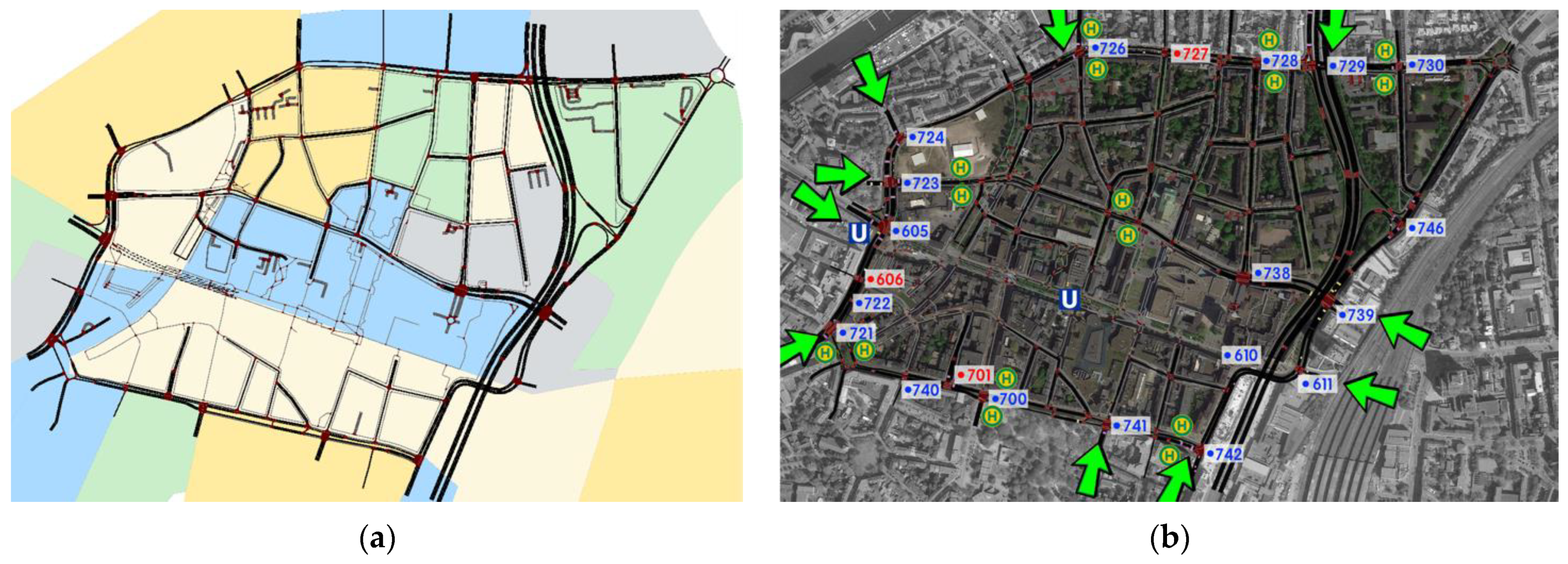
Figure 2a shows the partition of the OD matrix of Duisburg’s inner ring. There are 18 parts with roads in the inner ring and these parts are shown in five colors. Shown in Figure 2b is the induction loops distribution of this area. As the induction loops here are normally located in the intersections, all the intersections with traffic lights are marked with their intersection numbers. The blue numbers stand for fixed traffic light control intersections, and the red numbers represent dynamic traffic light control intersections. Unfortunately, not all the roads around each intersection have installed induction loops; the green arrows in the figure represent the in-city direction roads equipped with induction loops. In this figure, the bus stations and subway stations are also marked with H and U, respectively. There are, in total, 16 bus lines and 3 subway lines that pass through this area.
In this work, both traffic demand data sources are used in generating traffic, and the generated traffic volumes are compared with actual induction loops data. Public transportation, such as bus and subway, is neither included in the OD matrix data source nor the induction loops data. Therefore, in our simulation, the emphasis is placed on passenger cars.

2.3. Vehicle Models with Different Levels of Automation

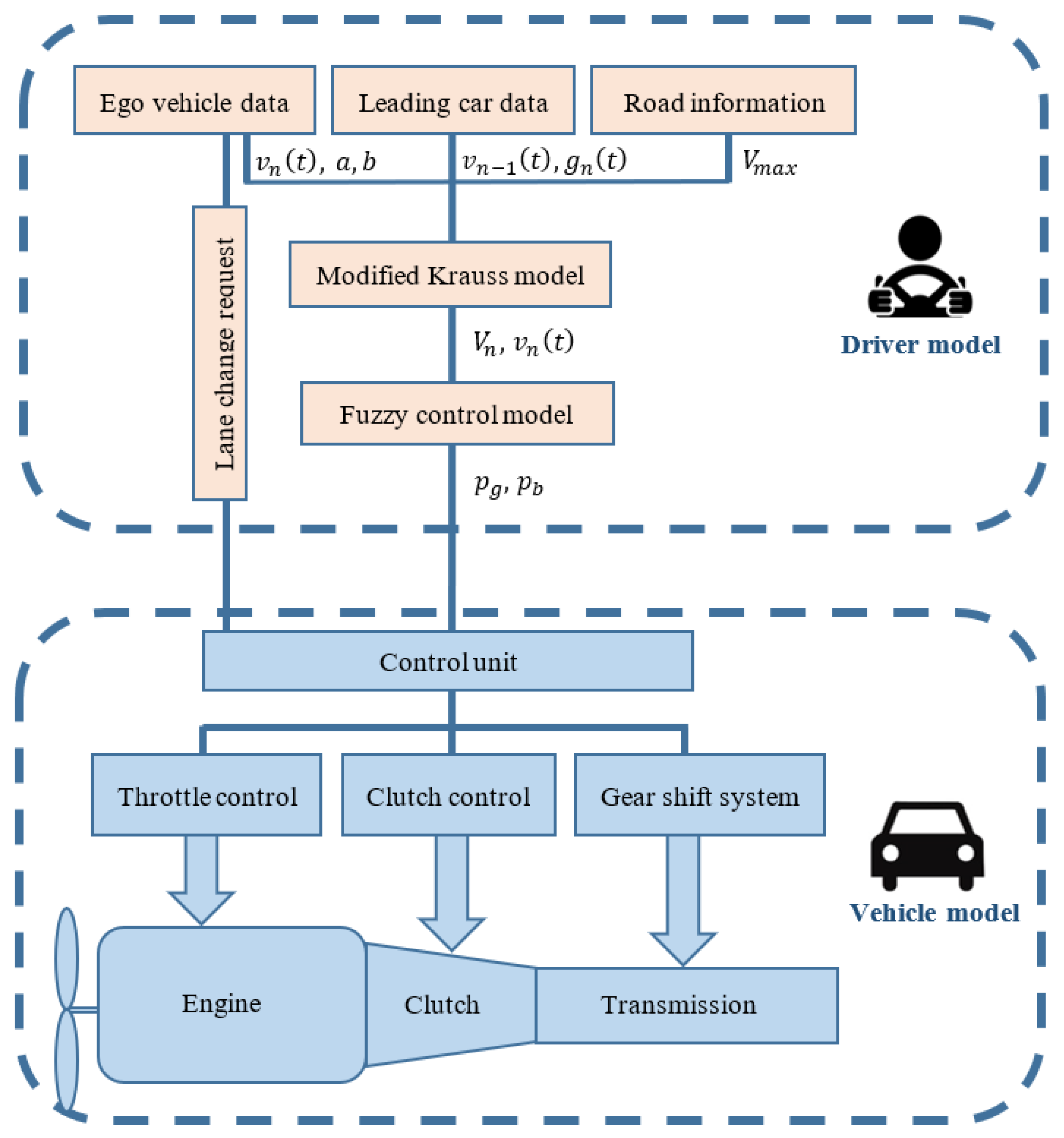
In this work, a driver–vehicle separate model is used for simulation. An obvious benefit of this kind of model is its flexibility. The driver model can be combined with different vehicle models (fuel, electric, hybrid, etc.), and the vehicle model can also combine with different driver models (autonomous driver, human driver, aggressive driver, etc.). As can be seen in Figure 3, driver model and vehicle model are independent of each other and connected by data transmission. The driver model simulates the reaction of a human driver on the road. Depending on the situation of the ego vehicle, leading vehicle, and other road information, the human driver/driver model controls the vehicle with a suitable gas/brake pedal position. In the car-following models of microscopic traffic simulation, the Krauss model has fewer conflicts with the lane-changing model because of its simplicity [26]. The driver model in this work consists of two parts. The modified Krauss car-following model [27] generates the desired speed of the driver, and the fuzzy control model outputs the gas/brake pedal position depending on the desired speed of the driver and the actual speed of the vehicle. The modified Krauss model can be expressed as:
{ v ( t + t l ) = max ( 0 , V n ϵ   a   η ) V n = min [ v s ,   V m a x , v n ( t ) + a n t l ] v s =   τ   b + ( τ   b ) 2 + v n 1 ( t ) 2 + 2 b   g n ( t ) x ( t + 1 ) = x ( t ) + v n ( t )   t l
where v ( t + Δ t ) represents the speed of the ego vehicle after time Δ t , V n is the desired speed, φ is a random perturbation to allow for deviations from optimal driving, ϵ is the imperfection factor of the driver, a is the acceleration of the ego vehicle, η is a random number between 0 and 1, v s is the safe speed, V m a x is the allowed speed of the road, v n ( t ) is the speed of the ego vehicle at time t , a n is the maximum acceleration, t l is the time step of the simulation,   τ is the reaction time of the driver, v n 1 ( t ) is the speed of the leading vehicle, b is the maximum deceleration of the ego vehicle, g n ( t ) is the gap between the leader and the follower, x ( t ) is the position of the ego vehicle at time t , and x ( t + 1 ) is the position of the ego vehicle at the next time step.
The fuzzy control model is established by a driving experiment with 34 human drivers in a driving simulator [19]. Based on the data transferred from the modified Krauss model, the desired speed of the driver V n and the actual speed of the vehicle v n ( t ) , the fuzzy control model outputs gas pedal position p g or brake pedal position p b with human-like fuzzy rules. The vehicle model considers the characteristic of the vehicle transmission and the driving resistances and is optimized by the data from the driving experiment.
Different levels of automation are reflected in the parameters of the modified Krauss model and fuzzy control model. Three degrees of automation are selected in representing the vehicle automation level of the current stage, as well as in the near future and the far-distant future. Considering the driver assistance functions of high-selling vehicles and the current automation level of vehicles on the road, Level 0 (no automation) is selected for the current stage. Level 2 (partial automation level) and Level 5 (fully autonomous vehicle) are selected for the automation levels in the near future and far-distant future, respectively. In order to effectively distinguish the difference between Level 0 and Level 2, it is assumed that, in the simulation, Level 2 vehicles are in the driving assisted mode. According to the different operators (human or machine) of reaction tasks at different levels, the reaction time τ of the driver is set to 1, 1, 0.5 for Level 0, Level 2, and Level 5, respectively, in the modified Krauss model. The randomness factor r is set to 0.5, 0, 0, respectively, for the three separate levels of automation in the fuzzy control model, in representing the random driving behavior of human driver compared to the machine driver. Under safety considerations, the speed limit of autonomous vehicles is adjusted. High driving speed will lead to a sharp increase in the number and severity of traffic accidents [28]. Therefore, the Level 5 driver models in this work have a lower speed limit compared to the Level 0 and Level 2 vehicles.

3. Establishment of Simulation

In order to simulate the Duisburg inner ring with vehicles of different degrees of automation, an open-source microscopic traffic simulation software SUMO (Simulation of Urban MObility) [29], developed by the German Aerospace Center (DLR), is used in this work. Compared to similar simulation software, SUMO has more possibilities of model extension with less complexity. Software with high complexity would have negative impacts with other models (such as the lane changing model, dynamic assignment model, etc.) which are not easy to be resolved [26]. Hence, the SUMO simulation package is selected in this paper for simulation with both data sources mentioned in 2.2.

3.1. OD Matrix Traffic Demand

In the process of generating traffic demand from the OD matrix, the traffic volume from the divided area (with different colors in Figure 2a) is assigned to roads in the area. As the OD matrix data source used in this work describes the total traffic volume in 24 h, there is no more specific data for the traffic volume per hour. Common daily timelines retrieved from cities in West Germany are used [30]. For passenger cars and trucks, timelines named TGw2_PKW and TGw_LKW are used separately for describing the traffic distribution on a workday. The overall process of generating traffic demand from the OD matrix is listed below:
  • Areas described by the OD matrix transfer into polygons in SUMO: The areas described by the OD matrix data source are saved in shapefiles (a data format for geometric location information); they are also described by geometric information (longitude and latitude). The most similar data format in SUMO is polygons. The boundary lines can be also described by geometric points in order. In this step, polyconvert in SUMO is used to transfer shapefiles into polygons.
  • Polygons to TAZ: The Traffic Assignment Zone (TAZ) is a district defined in SUMO and the vehicles can be coded to drive from one TAZ to another within a certain period. The TAZ also comprises districts constituted by points; for better visualization, the geometric coordinate format is transferred to the XY coordinate in SUMO. Figure 4 shows the TAZ distribution of the studied area; all the areas in OD matrix are marked with red boxes.
  • TAZ to edges/roads: To distribute the traffic demand from the whole zone into edges/roads, a python program called edgesInDistricts.py is used. Depending on the length of the roads, the traffic demand is distributed with different weights.
  • OD matrix to trips: After the scope-related work is done, the traffic volume is processed. A function called od2trips has been used. The timeline has been used here to assign traffic into hours. Trucks and passenger cars are processed separately.
  • Trips to routes: At last, through the network file and trip files in the last step, duarouter is used to generate the route file. The route file describes when and where each vehicle starts on the map, and through which edges/roads it arrives at the destination.

3.2. Induction Loops Traffic Demand

The induction loops data source consists of two parts: position and amount. The position file is in pdf format and the induction loops must be manually added into the network file in SUMO one by one. The amount file is in a machine-readable format. Unlike the method mentioned above, in this section, a fixed route, with the route file and vehicle file, are used. The route file describes the edges/roads a vehicle passes along, and the vehicle file represents the departure time, position, speed, and route of each vehicle. The process of generating traffic demand from induction loop data is listed below:
  • Loop position and type: There are three types of induction loops in SUMO; “source” loops are the ones where vehicles start, “between” loops are in the middle position, and “sink” loops are the loops where vehicles vanish from the simulation. In this paper, the roads outside the ring in the entering directions are selected to be the source loops. In total, induction loops on 8 roads marked with green arrows in Figure 2b are set as the source loops.
  • Traffic flow: In order to be recognized by the program, the flow file in SUMO should be in csv format with fixed form. However, the vehicle amount of each induction loop is saved by intersection names. MATLAB is used here to transform the data into the SUMO-required format.
  • Generate route files and vehicles: Using the network file and flow file, the route file and vehicle file required in the simulation are generated by a sub-program in SUMO called flowrouter. In this step, the departure lanes are also modified to avoid conflicts by generating routes.
  • Change source loops position: The positions of induction loops are always close to an intersection. Sometimes the distance between the induction loops is less than the length of a vehicle. This causes unwanted traffic jams upon vehicle insertion, which in turn affects the entire simulation. Therefore, all the positions of source loops are moved to the side, far from the intersection.
The induction loop data of a coherent week in 2019 are provided. However, some intersections have no data in the given period, some intersections have no installed induction loops, and data from one intersection are not usable due to a malfunction. Therefore, the induction loops used as source loops are adjusted according to the data situation. Finally, the induction loops used for source are marked with green arrows in Figure 2b. In total, 24 induction loops on 12 roads are selected to be the source loops. Each road has 1–3 lanes and each lane has one source induction loop. A total of 76 induction loops with valid data are used as traffic volume sources.

3.3. Verification Data

In order to verify the generated traffic volume from the OD matrix data and induction loops data, 4 verification points (V1–V4) on 4 roads are selected. These verification points are also induction loops near intersections. V1 belongs to intersection 727, in the west to east direction; the road with the induction loops has only one lane. V2 and V3 are in intersection 723; V2 records the vehicles from north to south while V3 records the vehicles from south to north. V2 has 3 lanes; only the two lanes with valid data are selected for the verification. V3 has 3 lanes, all of which are recorded. V4 belongs to intersection 742; the direction is from north to south. There are two lanes of this road section, and both are recorded. In total, 4 verification points with 8 induction loops are selected, covering the north, south, west, and east roads of the inner ring area of the scenario. Due to the data source of the OD matrix being 24 h, the simulated time of the two data sources is also set to 24 h. Furthermore, the verification data are also extracted for 24 h.

4. Results and Discussion

First, the accuracies of the traffic demand generated from different data sources (OD matrix and induction loops) are compared in Section 4.1. With the better data source, simulations of vehicles with different degrees of automation are carried out in Section 4.2. The results and comparison of the simulations are then introduced.

4.1. Comparison of Different Traffic Demand Sources

Figure 5 and Figure 6 show the traffic volume determined with the simulation settings presented in the last section and the average speed at the four verification points. The red lines represent the real data recorded by the induction loops. The blue lines show the simulation results from Section 3.2 and the black lines represent the simulation results from Section 3.1. From left to right, the four figures represent the four verification points from V1 to V4, respectively. In order to reduce the interference of different lane choices, the traffic volume is the sum of different lanes on the same road.
As can be seen in Figure 5, the blue lines are closer to the red lines than the black lines. That means, for the number of vehicles in the simulation, the simulation using induction loops data as the source of traffic demand has better results than the simulation using the OD matrix data. The reason could be that the OD matrix data only contains the trips that start or end in the range of the inner ring, and the trips passing by this area are not included. For V2 and V3, the difference between actual traffic volume and the OD matrix generated traffic volume is more significant than V1 and V4. The reason could be that most vehicles passing intersection 723 do not need to enter the inner ring area. This location of the intersection also proves that it bears more out-of-region traffic.
For the average velocity comparison in Figure 6, the simulation results using OD matrix data as traffic demand are closer to the real data at 24 h for a day. In contrast, the average speeds of simulation using induction loops data and OD matrix data are similar; sometimes lower than the real data, and sometimes higher. The zero average speed represents that there is no vehicle passing the verification point during this hour. The two simulations use the same traffic scenario and the same network file. Hence, the speed limit of the roads is also the same.
The deviation of the detector simulation data and the real data in traffic volume is σ = 37.43, which is better than the deviation of the OD matrix simulation data and the real data, which is σ = 129.20. Regarding velocity, the deviation of the detector’s data is σ =   7.44, and therefore slightly better than the deviation of the OD matrix, which is σ = 8.72. According to the comparison of simulation results, the simulation using induction loops data have a more realistic result than the simulation using the OD matrix in the aspect of traffic volume. The reason might be that the induction loops data record every vehicle passing by, but the OD matrix data only generates the vehicles that depart or end their journey at the selected area. In the next section, the induction loops data are also used as the traffic demand source for the simulation of vehicles with different degrees of automation.

4.2. Comparison of Different Degrees of Automation

To verify the effects of vehicles with different degrees of automation, vehicles of automation Level 0 (no automation), Level 2 (partial automation), and Level 5 (fully autonomous) are simulated in the traffic scenario of Duisburg inner ring. In this simulation, the number of vehicles, vehicle routes, departure time, and departure location on the network are the same, and only the degree of automation is varied. The simulation is for 24 h of a day, and the traffic demand is generated from the close-to-reality results of road detectors. To observe more details in the change of traffic volume, the data collection time cycle of verification detectors is changed to 600 s. The simulation results can be seen in Figure 7 and Figure 8; the average speed of vehicles in the simulation are shown separately (Figure 7) and in comparison (Figure 8). For the same traffic volume input, the vehicles with a higher automation level, represented by the red and blue lines in Figure 8, show a higher average speed than the vehicles without automation, represented by the black lines. In this simulation, the traffic status represents the real traffic situation of the Duisburg inner ring for a certain day. For the current traffic volume, vehicles in all three simulations can finish the driving task with average speeds close to the speed limits of the roads.
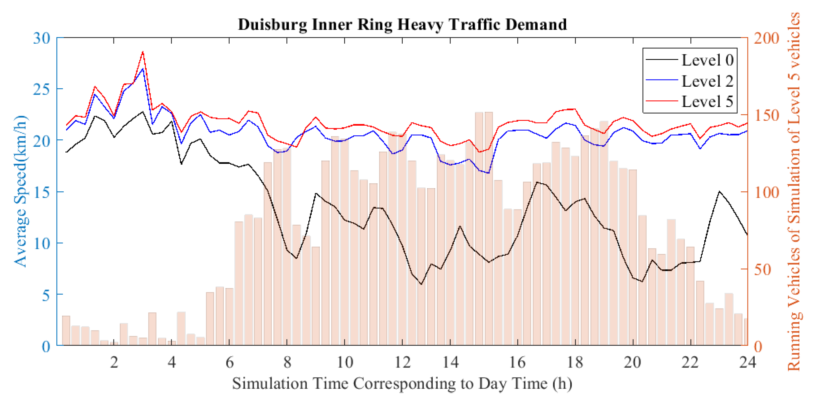
To create a heavy traffic demand situation, an extra 50% traffic volume is added to the scenario. If traffic conditions continue to deteriorate, there will be more vehicles on the road in the future, whether automated vehicles can improve the congestion problem or not. Figure 9 shows the average speed of vehicles in three different scenarios with Level 0, Level 2, and Level 5 vehicles. For the same heavy traffic volume input, the average speed of vehicles in the simulation with Level 0 vehicles is greatly affected (black line) and, in the other two simulations with vehicles of higher automation levels, the average speed is only slightly lower as in real traffic volume input. The simulation results show that, whether in the actual traffic volume or the possibly more congested future traffic situation, automated vehicles have a positive impact on the traffic flow. Vehicles with higher automation levels can take on more congested traffic conditions.

5. Conclusions and Discussions

In this work, a traffic scenario of Duisburg city inner ring has been built, and traffic demand of two different data sources has been generated and compared. In the four selected verification points, the traffic volume generated from induction loop data has a better reproduction ( σ = 37.43, compared to real data) than the OD matrix data ( σ = 129.20, compared to real data). Vehicles with different automation levels (Level 0/no automation, Level 2/partial automation, and Level 5/fully autonomous) are simulated continuously in the Duisburg city inner ring scenario for 24 h of a day. Based on the real traffic volume collected in 2019, the vehicles with automation Level 2 and Level 5 have positive effects on traffic. For more congested traffic status, the positive effects of vehicles with higher automation levels are more obvious.
This article uses a real scenario, the inner ring area of the city of Duisburg, as the traffic simulation scenario. Two kinds of data sources are provided for this article, and traffic demand generated from the two kinds of data sources are used separately. In the selected simulation scenario, induction loops data show better accuracy in reproducing the traffic. In this article, vehicles with different degrees of automation are simulated in the scenario. With the same traffic demand, highly automated vehicles can effectively increase average speed. In the case of increased road congestion (150% traffic volume), the increased average speed of automated vehicles is more obvious.

Author Contributions

X.M.: conceptualization, data curation, formal analysis, methodology, software, writing and editing. X.H.: conceptualization, methodology, software, validation, writing and editing, T.W. & D.S.: conceptualization, project administration and supervision, result validation and critical revision. All authors have read and agreed to the published version of the manuscript.

Funding

This research received no external funding.

Institutional Review Board Statement

Not applicable.

Informed Consent Statement

Not applicable.

Data Availability Statement

Restrictions apply to the availability of these data. Data was obtained from Duisburg city officials and the WBD and are available from the authors with the permission of Duisburg city officials and the WBD.

Acknowledgments

We acknowledge support by the Open Access Publication Fund of the University of Duisburg-Essen.

Conflicts of Interest

The authors declare no conflict of interest.

References

  1. United Nations. 2018 Revision of World Urbanization Prospects; United Nations: New York, NY, USA, 2018. [Google Scholar]
  2. Kalra, N.; Groves, D.G. The Enemy of Good: Estimating the Cost of Waiting for Nearly Perfect Automated Vehicles; Rand Corporation: Santa Monica, CA, USA, 2017; ISBN 1977400019. [Google Scholar]
  3. Blincoe, L.; Miller, T.R.; Zaloshnja, E.; Lawrence, B.A. The Economic and Societal Impact of Motor Vehicle Crashes, 2010 (Revised). Ann. Emerg. Med. 2015, 66, 194–196. [Google Scholar] [CrossRef]
  4. Fagnant, D.J.; Kockelman, K. Preparing a nation for autonomous vehicles: Opportunities, barriers and policy recommendations. Transp. Res. Part A Policy Pract. 2015, 77, 167–181. [Google Scholar] [CrossRef]
  5. Wadud, Z.; MacKenzie, D.; Leiby, P. Help or hindrance? The travel, energy and carbon impacts of highly automated vehicles. Transp. Res. Part A Policy Pract. 2016, 86, 1–18. [Google Scholar] [CrossRef] [Green Version]
  6. Marshall, A. After peak hype, self-driving cars enter the trough of disillusionment. Wired, 29 December 2017. [Google Scholar]
  7. Philanthropies, B. Is your city getting ready for AVs. This is a guide to who’s doing what, where, and how. Hentet 2018, 12, 18. [Google Scholar]
  8. Kerry, C.F.; Karsten, J. Gauging Investment in Self-Driving Cars; Retrieved 28 November 2017; Brookings: Washington, DC, USA, 2017. [Google Scholar]
  9. Lanctot, R. Accelerating the Future: The Economic Impact of the Emerging Passenger Economy; Strategy Analytics: Boston, MA, USA, 2017; Volume 5, 30p. [Google Scholar]
  10. Nunes, A.; Hernandez, K.D. Autonomous Vehicles and Public Health: High Cost or High Opportunity Cost? Transp. Res. Part A Policy Pract. 2019, 138, 28–36. [Google Scholar] [CrossRef]
  11. Green, W.H.; Armstrong, R.C.; Ben-Akiva, M.; Heywood, J.; Knittel, C.; Paltsev, S.; Reimer, B.; Vaishnav, C.; Zhao, J.; Gross, E. Insights Into Future Mobility: A Report from the Mobility of the Future Study. 2019. Available online: http://energy.mit.edu/publication/insights-into-future-mobility/ (accessed on 20 December 2020).
  12. Peters, P.L.; Kröger, L.; DeMuth, R.; Schramm, D. Derivation of scaled design premises for future vehicle concepts based on a forecast of travel demand using the example of a commercial fully automated on-demand fleet. Automot. Engine Technol. 2019, 4, 45–61. [Google Scholar] [CrossRef]
  13. Vlakveld, W.P. Transition of Control in Highly Automated Vehicles: A Literature Review; SWOV: Hague, The Netherlands, 2016. [Google Scholar]
  14. Zohdy, I.; Kamalanathsharma, R.; Sundararajan, S.; Kandarpa, R. Automated Vehicles from Modeling to Real World. Road Vehicle Automation 2; Springer: Berlin, Germany, 2015; pp. 187–191. [Google Scholar]
  15. Van Arem, B.; Van Driel, C.J.G.; Visser, R. The Impact of Cooperative Adaptive Cruise Control on Traffic-Flow Characteristics. IEEE Trans. Intell. Transp. Syst. 2006, 7, 429–436. [Google Scholar] [CrossRef] [Green Version]
  16. Reece, D.A.; Shafer, S.A. A computational model of driving for autonomous vehicles. Transp. Res. Part A Policy Pr. 1993, 27, 23–50. [Google Scholar] [CrossRef]
  17. Talebpour, A.; Mahmassani, H.S.; Bustamante, F.E. Modeling Driver Behavior in a Connected Environment: Integrated Microscopic Simulation of Traffic and Mobile Wireless Telecommunication Systems. Transp. Res. Rec. 2016, 2560, 75–86. [Google Scholar] [CrossRef]
  18. Talebpour, A.; Mahmassani, H.S.; Elfar, A. Investigating the Effects of Reserved Lanes for Autonomous Vehicles on Congestion and Travel Time Reliability. Transp. Res. Rec. 2017, 2622, 1–12. [Google Scholar] [CrossRef]
  19. Ma, X.; Hu, X.; Schweig, S.; Pragalathan, J.; Schramm, D. A Vehicle Guidance Model with a Close-to-reality Driver Model and Different Levels of Vehicle Automation. Appl. Sci. 2021, 11–380. [Google Scholar] [CrossRef]
  20. Organisation for Economic Cooperation and Development. Population by Region—Urban Population by City Size—OECD Data. Available online: https://data.oecd.org/popregion/urban-population-by-city-size.htm (accessed on 18 May 2020).
  21. Giffinger, R.; Fertner, C.; Kramar, H.; Meijers, E. City-ranking of European medium-sized cities. Cent. Reg. Sci. Vienna UT 2007, 1–12. Available online: http://www.smart-cities.eu/model.html (accessed on 18 June 2008).
  22. Kunzmann, K.R. (Ed.) Medium-Sized Towns, Strategic Planning and Creative Governance. In Making Strategies in Spatial Planning; Springer: Berlin, Germany, 2010; pp. 27–45. [Google Scholar]
  23. Bergan, P.; Mölders, A.-M.; Rehring, K.; Ahlemann, F.; Decker, S.; Reining, S. Towards Designing Effective Governance Regimes for Smart City Initiatives: The Case of the City of Duisburg. In Proceedings of the 53rd Hawaii International Conference on System Sciences, Maui, HI, USA, 7–10 January 2020. [Google Scholar]
  24. Alessandrini, A.; Campagna, A.; Delle Site, P.; Filippi, F.; Persia, L. Automated Vehicles and the Rethinking of Mobility and Cities. Transp. Res. Procedia 2015, 5, 145–160. [Google Scholar] [CrossRef] [Green Version]
  25. Willumsen, L.G. Estimation of an OD Matrix from Traffic Counts–A Review; University of Leeds: Leeds, UK, 1978. [Google Scholar]
  26. Bjärkvik, E.; Fürer, F.; Pourabdollah, M.; Lindenberg, B. Simulation and Characterisation of Traffic on Drive Me Route around Gothenburg using SUMO. In Proceedings of the SUMO User Conference 2017, Berlin, Germany, 8–10 May 2017. [Google Scholar]
  27. Krauss, S. Microscopic Modeling of Traffic Flow. Investigation of Collision Free Vehicle Dynamics; Als Ms. gedr; Dt. Zentrum für Luft- und Raumfahrt e.V., Abt; Unternehmensorganisation und -Information: Köln, Germany, 1998. [Google Scholar]
  28. Richards, D.C. Relationship between Speed and Risk of Fatal Injury: Pedestrians and Car Occupants; Transportation Research Laboratory, Department of Transport: London, UK, 2010. [Google Scholar]
  29. Lopez, P.A.; Behrisch, M.; Bieker-Walz, L.; Erdmann, J.; Flötteröd, Y.-P. Microscopic traffic simulation using sumo. In Proceedings of the 2018 21st International Conference on Intelligent Transportation Systems (ITSC), Maui, HI, USA, 4–7 November 2018. [Google Scholar]
  30. Schmidt, G.; Thomas, B. Hochrechnungsfaktoren für manuelle und automatische Kurzzeitzählungen im Innerortsbereich. In Forschung Straßenbau Straßenverkehrstechnik; Bundesministerium für Verkehr: Bonn, Germany, 1996. [Google Scholar]
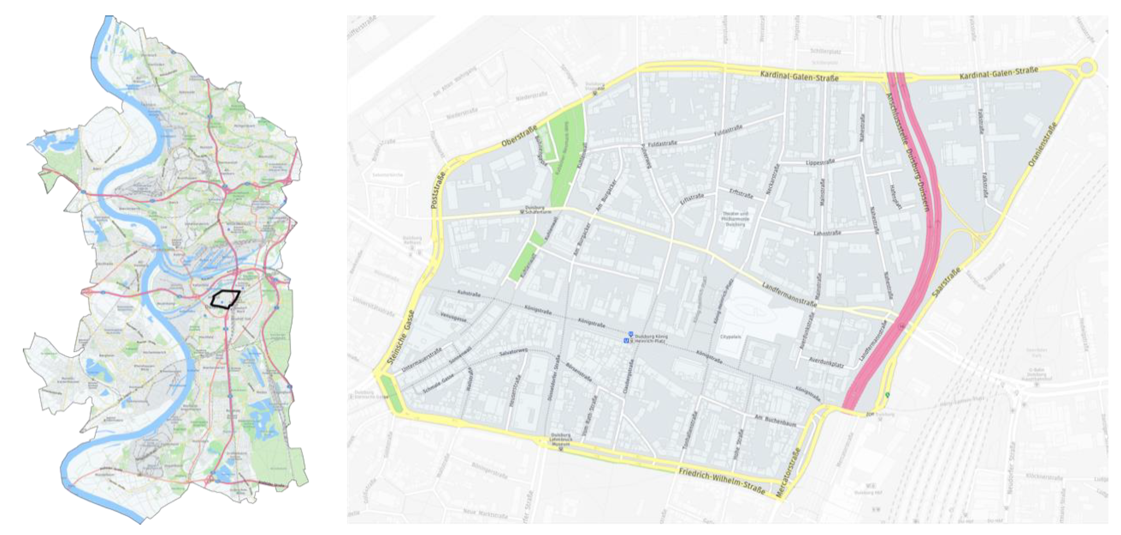
Figure 1. The location of Duisburg inner ring (Source: Here map).
Applsci 11 00029 g001
Figure 2. Two data sources of traffic demand ((a) Origin–Destination (OD) matrix, where the distribution of OD areas is shown in different colors; (b) induction loops, where the numbers are intersections of the inner ring area).
Applsci 11 00029 g002
Figure 3. Driver–vehicle model in this work.
Applsci 11 00029 g003
Figure 4. Traffic Assignment Zone (TAZ) distribution of Duisburg inner ring; each red box shows the roads in one TAZ.
Applsci 11 00029 g004
Figure 5. Traffic volume of the verification points. (Red lines, real data; blue lines: simulation of intersection loops data; black lines: simulation of OD matrix data).
Applsci 11 00029 g005
Figure 6. Average velocity of different hours in the verification points. (Red lines, real data; blue lines: simulation of intersection loops data; black lines: simulation of OD matrix data).
Applsci 11 00029 g006
Figure 7. Average speeds of vehicles and running vehicle numbers of simulations with vehicles of different automation levels.
Applsci 11 00029 g007
Figure 8. Comparison of average speeds of vehicles with different automation levels in real traffic volume (100% traffic volume).
Applsci 11 00029 g008
Figure 9. Comparison of the average speed of vehicles with different automation levels in heavy traffic volume (150% traffic volume).
Applsci 11 00029 g009
Publisher’s Note: MDPI stays neutral with regard to jurisdictional claims in published maps and institutional affiliations.