Identification of Tire Model Parameters with Artificial Neural Networks

Abstract

Accurate modeling of tire characteristics is one of the most challenging tasks. Many mathematical models can be used to fit measured data. Identification of the parameters of these models usually relies on least squares optimization techniques. Different researchers have shown that the proper selection of an initial set of parameters is key to obtain a successful fitting. Besides, the mathematical process to identify the right parameters is, in some cases, quite time-consuming and not adequate for fast computing. This paper investigates the possibility of using Artificial Neural Networks (ANN) to reliably identify tire model parameters. In this case, the Pacejka’s “Magic Formula” has been chosen for the identification due to its complex mathematical form which, in principle, could result in a more difficult learning than other formulations. The proposed methodology is based on the creation of a sufficiently large training dataset, without errors, by randomly choosing the MF parameters within a range compatible with reality. The results obtained in this paper suggest that the use of ANN to directly identify parameters in tire models for real test data is possible without the need of complicated cost functions, iterative fitting or initial iteration point definition. The errors in the identification are normally very low for every parameter and the fitting problem time is reduced to a few milliseconds for any new given data set, which makes this methodology very appropriate to be used in applications where the computing time needs to be reduced to a minimum.

1. Introduction

The identification of parameters in tire models has been addressed through different techniques. It is common practice in the literature to consider the cost function that takes into account only the vertical component of the error between measured data and the mathematical model, assuming indirectly that the independent variable is well known or, at least, that its contribution to the total error is negligible.

Historically, the most used methodology to identify tire model parameters has been the Ordinary Least Squares on the Pacejka’s Magic Formula (MF) model [1]. The most widely used methods have been derived from the different alternatives of Newton’s method [2]: Gauss–Newton, Levenberg–Marquardt [3], quasi-Newton [4], sequential quadratic programming SQP [5], Nelder–Mead [6], etc. A comparison of various algorithms can be found in [7]. Recently, a Weighted Orthogonal Regression method was presented to account for errors in the slip and the force values [8]. These methods are by their nature iterative and rely on a suitable starting point. In this case, this means that an appropriate initial set of parameters needs to be given to the algorithm to be able to provide a satisfactory solution. This is due to the fact that multiple local minima can be found in the cost function, and these Newtonian methods search for local minima.

An interesting alternative for the identification of these coefficients is to use Genetic Algorithms (GA) and Neural Networks (NN). GA has been found to be good at exploring the parameter space [9,10] and at estimating the MF coefficient, even starting from a bad estimation of the initial parameters. However, GA it is not very suitable for precise exploitation (i.e., identifying the optimum set of parameters). Recently, Talebitooti [11] has combined GA with a local search algorithm, proving that this hybrid two-step method is much more efficient.

ANN has been successfully used along with state observers for dynamic control of cars [12,13]. Palkovic and El-Gindy [14] investigated some applications of the ANN to vehicle dynamics and control and compared it to the MF. They used tire test data to directly train the ANN and the results were promising. However, the starting data for the network training was very limited, as it was based on data from individual tires, of which there was also little data available for the network training.

Regarding tire data obtained directly from the direct interaction of the tire with the road, Farroni [15] proposes a tool called TRICK to estimate the tire interaction forces as a function of slip rates, thus avoiding expensive and time consuming test bed characterizations. Later, Farroni [16] also proposed the use of another tool called TRIP-ID, for the interactive identification of tire parameters based on data from experimental bench data or direct interaction with the road. In the same way, Wang [17] presented the identification of parameters through ANN for a specific tire, based on real test data of a race car tire (Hoosier 18.0 x 6-10R25B) on a test bench for different test conditions.

In this line, in the evaluation of the parameters of Pacejka’s MF model in the road operation of tires based on data acquisition, there is the problem of not having continuous data in the whole range and combinations of the slips. Therefore, it would be necessary to combine this identification of partially observable data in the vehicle dynamic system (with noisy and/or incomplete acquired data) with methodologies to reconstruct the complete model, as proposed by [18].

Unlike previous studies into ANN identifying tire parameters in MF, the present study is based on the evaluation of the possibility of creating a widely valid ANN, which can be trained to predict the parameters of Pacejka’s MF, for a wide range of real tires. For this, a sufficiently ample database of curves is artificially created. Unlike previous ANN works, limited training data (due to data from only one, or a limited set of tires) is not a problem, since the methodology provides means to create as much training data as is necessary to ensure good network training. Based on this information, the ANN topology is selected and its performance is evaluated.

Therefore, this article presents a novel methodology to create a “universal” ANN-based mathematical model, which can be trained before knowing the specific data obtained from bench tests, or from the acquisition of data of the tire-road contact. Furthermore, this ANN can consider all the specific variations that the Pacejka curve admits, being therefore valid to represent any of the effects (pure-slip, combined-slip, camber angle, pressure, temperature, humidity, etc.) that make such a mathematical model vary. Obviously, since it is based on a mathematical model that may not be perfect (in the sense that it may not be exactly faithful to reality), the ANN obtained will have at least the same errors as the model it represents (in this case Pacejka’s MF). The advantage of having a pre-trained network that can represent a wide variety of conditions for different types of tires and immediately identify their Pacejka parameters is evident when you consider that the run time of such a network is only a few milliseconds. This low cost computation allows it to be integrated into real-time vehicle computer models, allowing identification from the data obtained from the vehicle, to have a system dynamic adaptable to the specific conditions and environmental variables of the tire on the vehicle.

The results shown in this paper are part of an ongoing research on the application of different technologies to the identification of vehicle system dynamic parameters [19]. The identification of parameters has also been extended to other mathematically simpler tire models [20] and the identification errors have also been small.

The study presented in this paper is organized as follows. Section 2 presents ANNs in general, their configuration and operation. Section 3 presents the methodology followed in this paper. Section 3.1 deals with the generation of sufficient data (without errors) to train the ANN. Selection of the topology of the ANN, its training and validation, are explained in Section 3.2. In Section 3.3, data (with errors) acquired in bench in tire tests are used to analyze the predictive performance of the network in real situations. Finally, in Section 4, final conclusions are exposed.

2. Artificial Neural Networks (ANNs)

The ANNs can be defined as processing algorithms that infer patterns and relationships between known input and output data, provided sufficient information is given to the system to learn. An ANN is set up mimicking the neural structure of the human brain, where hundreds of thousands of “simple” processor units (neurons) work together by interconnections among them (synapses) to allow learning. In this way, in one type of ANN, the network topology is composed of simple nodes that are organized in layers. The first layer usually has as many nodes as input parameters. The last layer is set up with as many nodes as output parameters (Figure 1).

Between these two layers there exist some hidden layers, each of them comprised of a given number of nodes. Nodes from two consecutive layers are usually fully connected between them. Each connection is given a weighting factor that is used to modify the information traveling through it. These connections allow passing information from one node to others connected to it. When the information is passed from left to right, it is called a “feed forward” connection. Nodes between consecutive layers can develop connections among them passing in this way information from one node to the other. Nodes sum up all the weighted information from their input connections in the previous layer and transmit the result to the output connections in the following layers.

To start the training process, after proper randomizing of the weights, the input layer of the ANN gets the input information from the algorithm and passes it on to the following layers. Each node receiving information acts on it and modifies it according to its activation configuration (normally a sigmoid, or similar function). In this way, the information travels through the ANN from the input nodes to the output ones. The training algorithm compares this result to the known solution of the provided training data. If the solution is not ok, then a so-called “backpropagation” algorithm modifies the weights of the connections according to the size of the error difference. Once the weights of all the connections have been updated, all the process is repeated until the answer given by the output layer is satisfactory (or a given stop flag is activated).

This procedure is called “supervised learning”, because one knows in advance the correct answer and, if the algorithm fails to obtain it, the ANN weights are corrected in order to get a better solution. Once the ANN has learned from the training data, it can provide solutions for unknown data. Therefore, the ANN is trained with the so-called “training data”, and its performance is usually measured by getting an answer from unknown “test data”. If the learning of the ANN has been successful, the answer to the “test data” will be satisfactory.

ANNs have already been used in a countless number of applications where analytical solutions do not exist or are very costly to obtain. There are many types of ANN. The configuration of the connections of ANNs is very dependent on the type of problem under study [21,22,23]. In order to build an efficient ANN, it is necessary to determine its type, topology and learning rule.

In this case, it is desired to know the optimum tire parameters related to the known test data of a particular tire. The input data will be the known test data for certain slips. In this paper, the input data to the network will be the longitudinal force measurements corresponding to slips ranging from −75% to 75%, discretized in steps of 2% for the slip. This gives us 76 entries to the network. These inputs are of a continuous character since the measured longitudinal force can have any continuous real value.

The output of the ANN are the parameters of the chosen tire model. In this case, it has been decided to work with the well-known Magic Formula [1], which is a semi-empirical tire model, and is the most used in the work related to tire models.

In its reduced form, the Magic Formula has six parameters that must be identified to know the whole curve. The output of the ANN will, therefore, have six outputs, one for each parameter. It is important to realize that this model (1) is very nonlinear since it has some nested trigonometric functions, which makes its complexity very high and, as will be seen, will affect the selection of the chosen ANN (see Section 3).

$$F_i=f_y+Fz·D\cdot \sin \left(C\cdot \arctan \left(B\cdot \left(x_i+f_x\right)-E\cdot \left(B\cdot \left(x_i+f_x\right)-\arctan \left(B\cdot \left(x_i+f_x\right)\right)\right)\right)\right)$$

(1)

The model (1) has the following nomenclature: xi is the longitudinal (or lateral) slip in % and Fi is the longitudinal (or lateral) force, in N. The pairs of values (xi, Fi) are known from tests performed on tire test benches. The remaining variables are the parameters that need to be identified. The parameter fx reflects the “horizontal shift” of the curve and fy the “vertical shift” that show the deviations in x and y from the curve that does not exactly pass through the coordinate origin. The parameter D is the peak factor, which multiplies to the Fz (vertical force on the tire). Both parameters together Fz·D stand for the maximum amplitude height of the curve. Parameter C represents the shape factor of the curve and B is the stiffness factor. Finally, the parameter E is the “curvature factor”.

Usually, ANNs are used for classification issues or discrete outputs. In this case, all the parameters to be identified are continuous variables, so it is necessary that the ANN support real-valued continuous output variables. The input and output data of the network are known, so a supervised training will be used. The ANN will be based on a Multi-Layer Perceptron (MLP), with nodes totally connected to each other between successive layers (Feed-Forward) [24], activated through the sigmoid function (with continuous derivative) that allows training through the Backpropagation Algorithm [21]. The selection of the chosen ANN topology is detailed in the following section as part of the working methodology.

3. Methodology and Results

In this paper, we intend to study the extent to which ANNs are adequate and could be used to predict the parameters of tire curves such as MF from known data from bench tests.

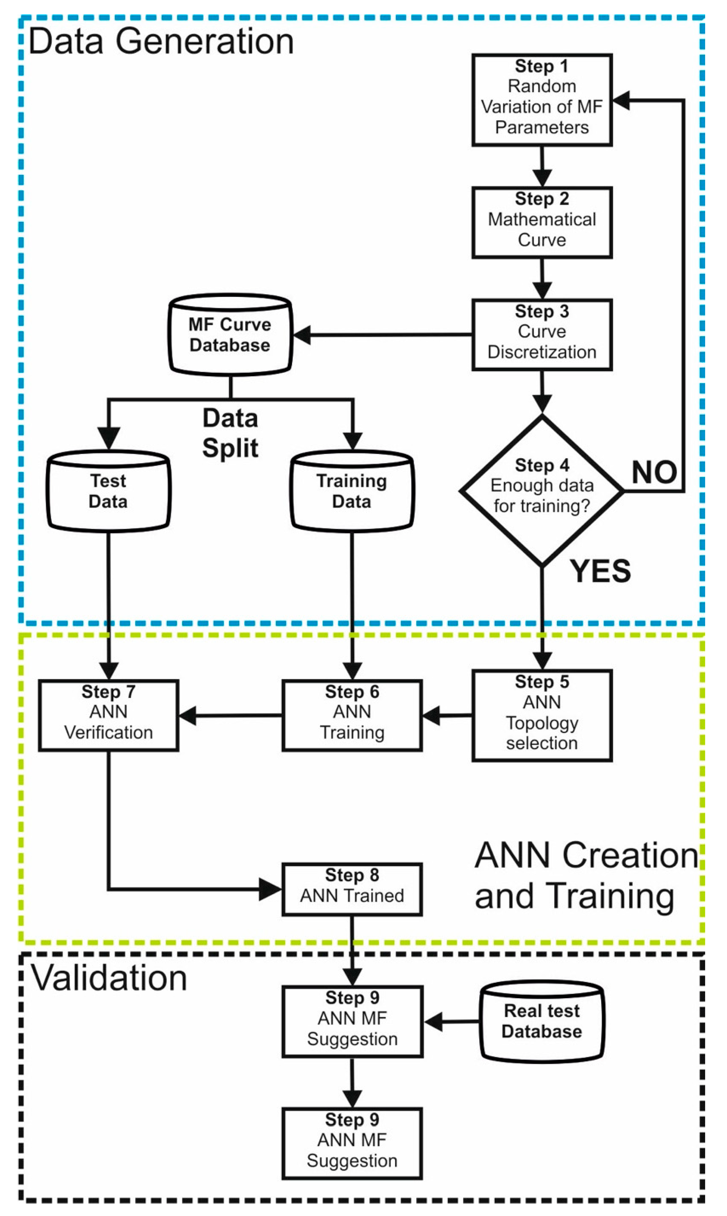
In order to answer this question, the work has been proposed according to the methodology shown in Figure 2, which is divided into three large blocks: (1) creation of curves to train the ANN; (2) determination of the topology of the ANN and its training; and (3) validation of the ANN against real test bench data.

In summary, this methodology intends to train the ANN from a sufficiently high number of known tire curves. The main problem is that conducting tests on real tires is very costly and it would not be economically feasible to carry out so many tests to train a universal ANN that can predict the parameters of the MF curve in all possible conditions and situations.

For this reason, the proposed methodology creates synthetic curves based on the use of the MF model. The idea is simple. Knowing the range of values in which the parameters f_x, f_y, B, C, F_z·D, and E can take in real tire curves, it is possible to generate a sufficiently large set of random combinations. In this way, it is possible to create as many curves as needed so that ANN training can be performed properly.

This is the purpose of the first part (Data Creation) of the methodology proposed in Steps 1 to 4 and explained in Section 3.1. The second part (ANN Creation and Training) studies the topology that the ANN must have to be able to adapt to the nonlinearity of the application (discussed in Section 3.2) and the ability of the trained network to predict the parameters of unknown synthetic curves (Steps 5 to 8). The third part (discussed in Section 3.3) examines the ANN’s ability to predict the parameters of unknown curves with measurement errors from actual tests on tire test benches (Steps 9 to 10).

3.1. Data Creation

The creation of synthetic data, from the mathematical model provided by the MF, is carried out in Steps 1 to 4 (Figure 2). First, in Step 1, the parameters of the tire model are varied randomly and independently of each other, in a sufficiently wide range of values to cover the largest possible combination of true tire curves. For this study, the limits of the values that these parameters can take are indicated in

Table 1. Range of values for MF model parameters.

Variable	Minimum	Maximum
xi	−0.75	+0.75
B	5	30
C	0.5	2
E	−2	0
Fz	1000	5000
D	0.1	2
fx	−0.02	0.02
fy	−300	+300

. It is important to note that the synthetic data obtained are free from errors arising from the application in which the tires are used (from test bench or vehicle dynamic system acquisition). However, it must be stressed that mathematical errors always exist in the model (either because the model chosen, in this case Pacejka’s model, does not perfectly match reality, or because of mathematical calculation errors, rounding or truncation).

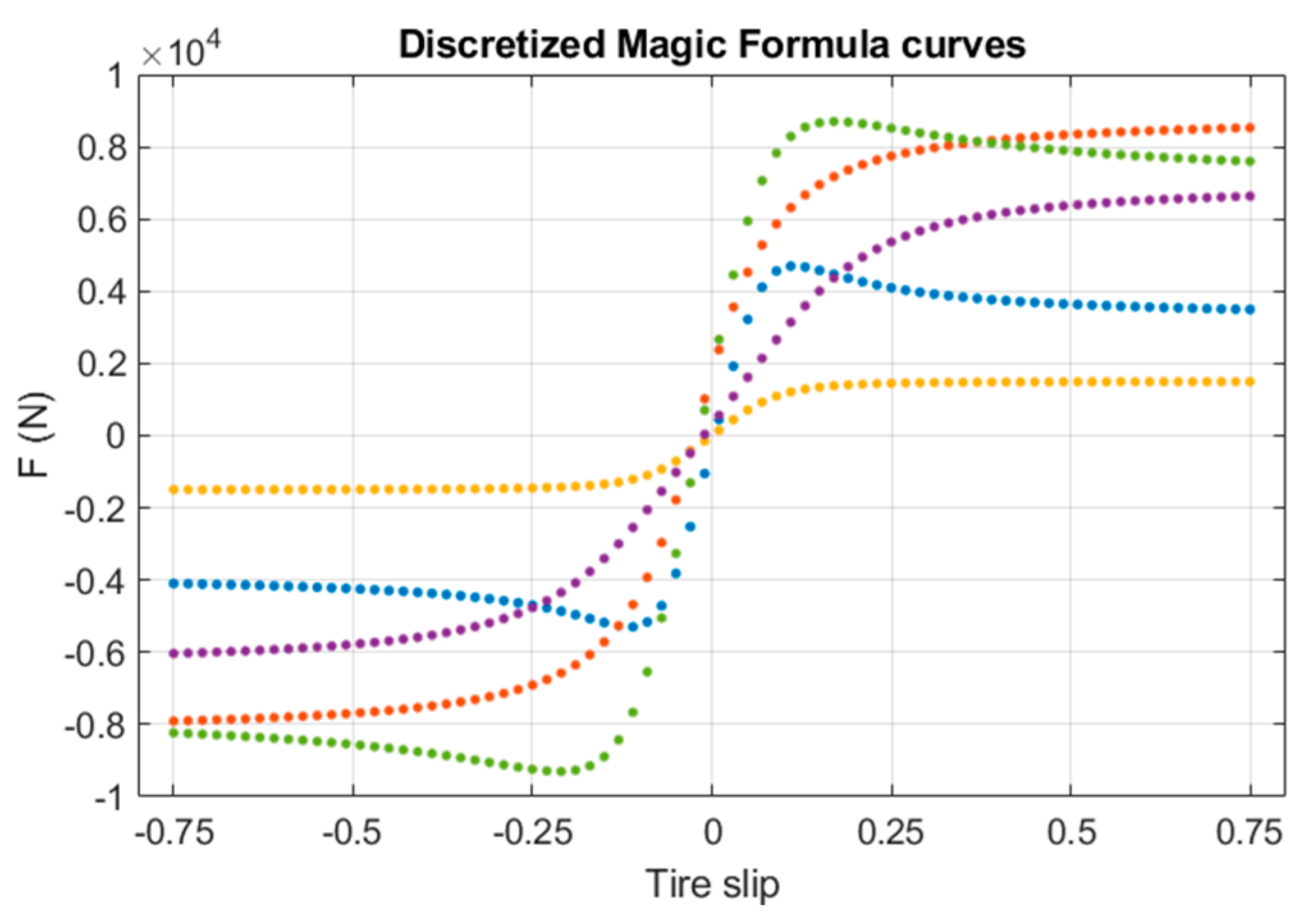
In Step 2, the mathematical curves are obtained. It can be noted that each set of random parameters produces a very different mathematical curve F_i. For example, in Figure 3, some different curves are shown from Equation (1) for different sets of random parameters.

It is important to remark that the range of the parameters has been selected to be sufficiently broad, so that the MF curve can have, mathematically, very different shapes.

In Step 3, the curves are discretized in 2% slip steps in the x_i slip range (e.g., Figure 4). These data points are saved in the training database together with the original set of MF parameters that produced the original curve. This information will be used later in the supervised training of the ANN.

It is important to note that the curves generated from the MF are mathematically perfect. That is, as they have been generated mathematically, there is no error in the parameters, the slip or the longitudinal/lateral force. This is very convenient at this point to be able to evaluate the ability of the ANN to represent a sufficiently complicated mathematical model without including other uncertainties or error variables.

One of the objectives of the ANN training is that the network learns to generalize the relationships between the parameters and the actual curve. This can be achieved if the training data is big enough. Step 1 to step 3 are repeated until sufficient data is gathered to train the ANN.

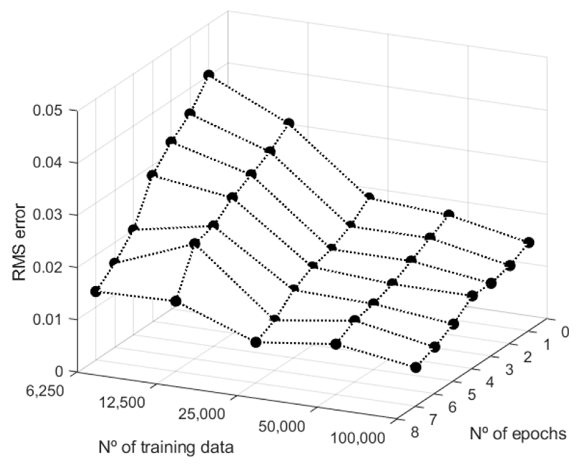
There are no fixed rules to define how many data sets are necessary to train an ANN successfully. This number depends on the complexity and non-linearity of the model under study. In order to be able to determine how big the data size needs to be, during the works in this investigation, the ANN has been trained with sets of a different number of curves and the training error was measured. Figure 5 shows the root-mean-square deviation (RMS Error) at the increasing number of curves in the training set and at a different number of training iterations (epochs). The trend shows that the higher the number of data sets the smaller the training error is. It can also be seen that the error is quite similar at 25k, 50k or 100k curves (with an RMS Error around 0.010 at 8000 epochs). In this study, to make sure a good training is achieved, a data set of 100k curves was selected (Step 4).

3.2. Ann Selection, Training and Validation

After the selection of the training data, we can move on to the second part of the methodology (Steps 5 to 8 in Figure 2), which focuses on the determination of the topology of the ANN (Step 5), its training (Step 6) and its verification (Step 7).

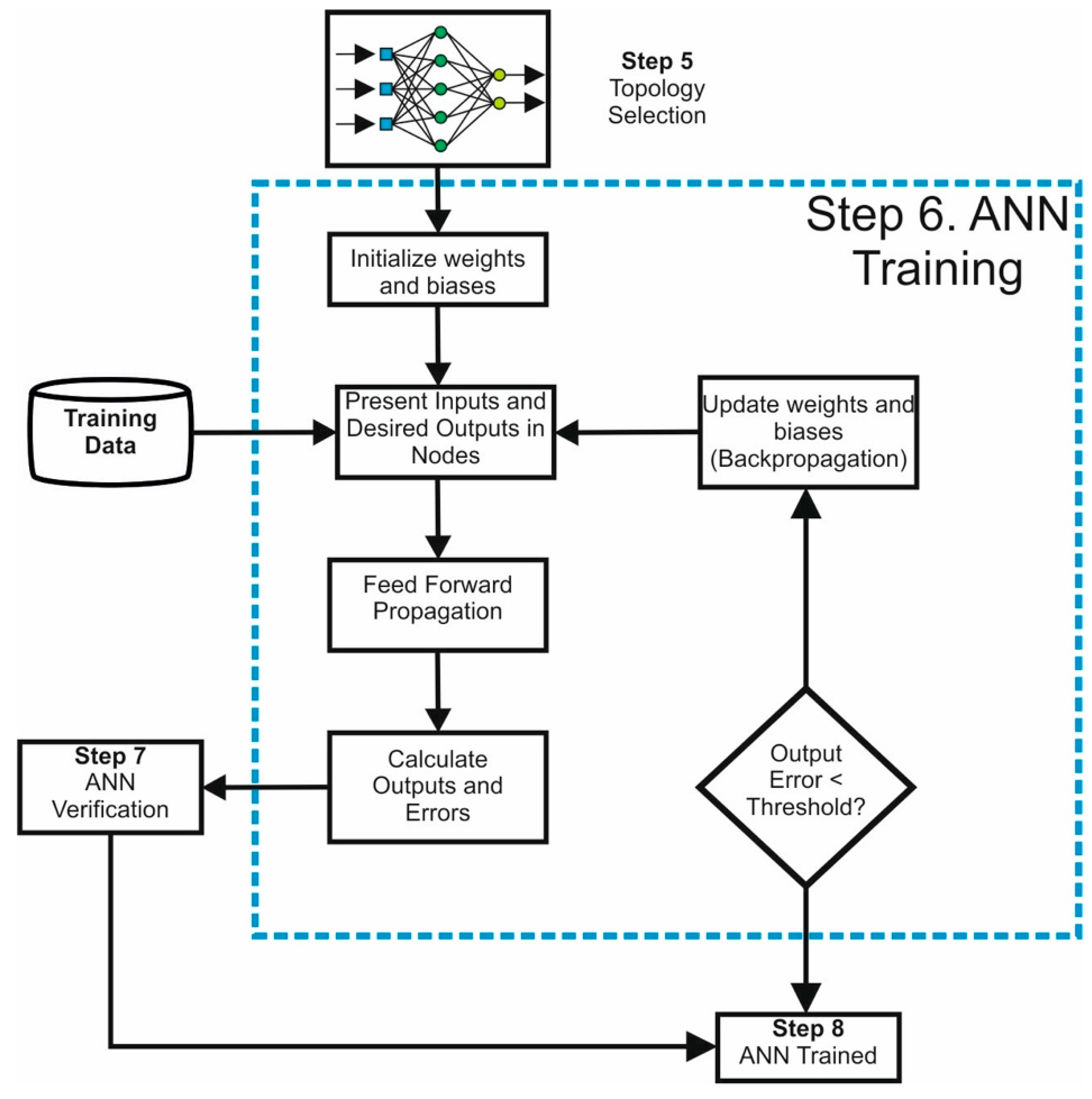
In Step 5 topology of the ANN is selected. This topology has to assure full connection between nodes of consecutive layers in the ANN. The selected learning rule type is supervised. Connection weights between neurons are updated in sequential training iterations according to the output targets and the obtained outputs.

For the hidden layers, different architectures may be valid and there is no general rule on how to obtain an optimum one as it depends on the complexity of the problem under study. Most of the literature suggests that from a theoretical point of view it is possible to approximate almost any function with one layer of ANN. If this is correct, it means that a single layer ANN with a sufficient number of hidden neurons can provide a good approximation for most problems. It also means that adding a second or third layer yields little benefit.

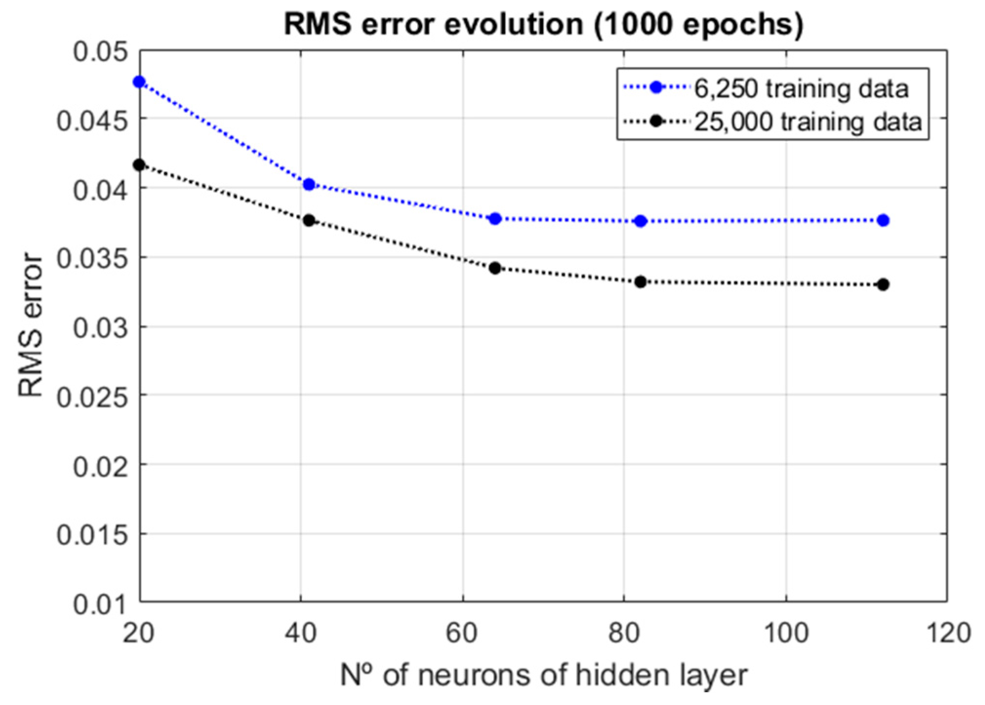
Following these recommendations, the possibility of using an ANN with a single hidden layer was explored. Figure 6 shows that more nodes on the hidden layer reduce the training RMS Error. This is true for different training data sets sizes (e.g., 6.25k or 25k). However, the improvement is very small despite continuing to increase the number of nodes in the network. Therefore, for this problem, it does not seem appropriate to use a single hidden layer ANN.

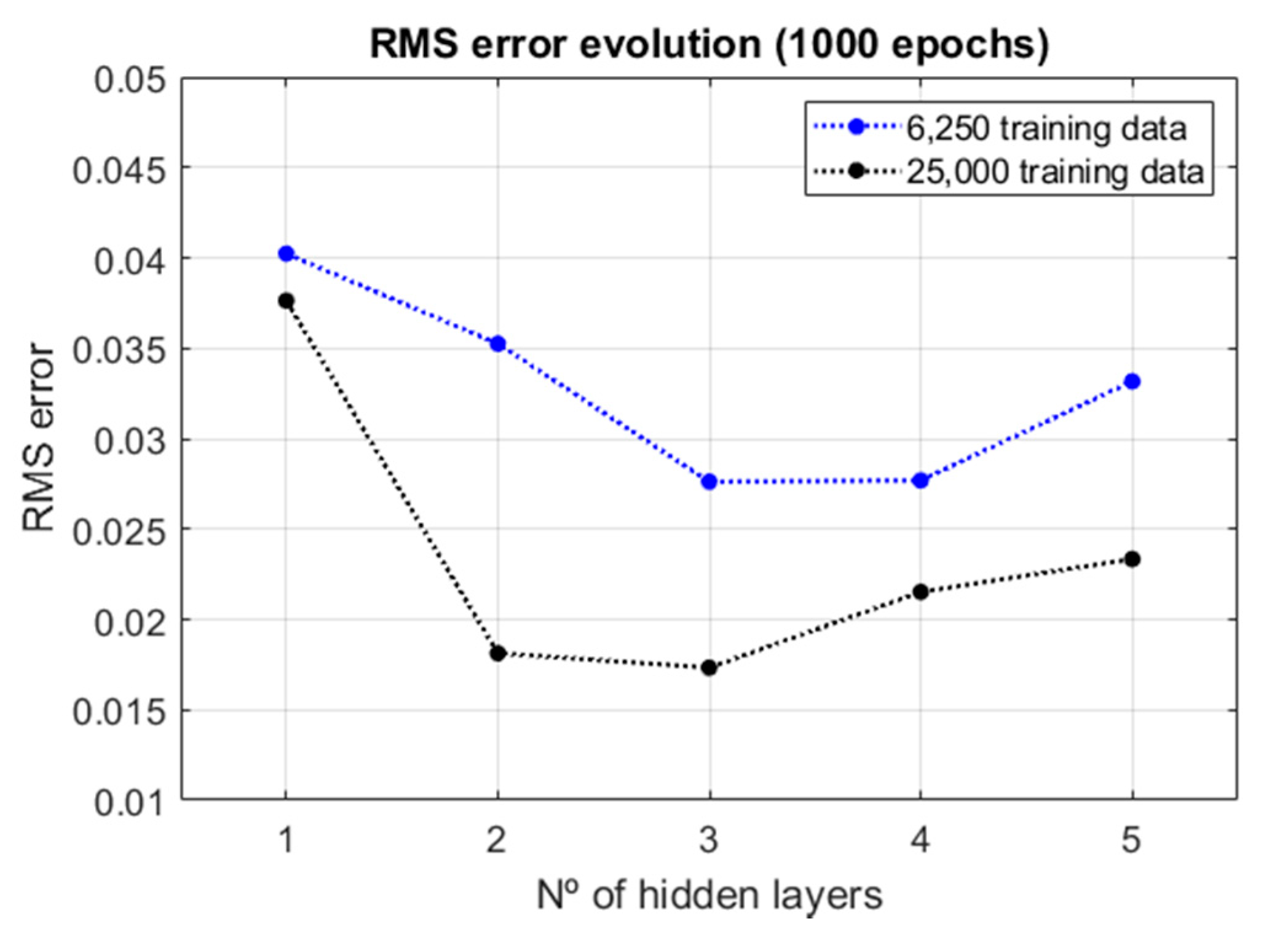
The identification of tire parameters is a highly non-linear problem. For this reason, a study was carried out in order to identify the best network topology that best suits this situation. Several network topologies were tested from one (1H) to five (5H) internal hidden layers with the same number of training curves (6.25k and 25k) running over 1000 iterations (epochs). The distribution of nodes within the network between successive hidden layers was done progressively so that the transition between the 76 inputs and the 6 outputs was “smooth”. The distribution of nodes was as follows: 76-41-6 (1H), 76-50-25-6 (2H), 76-50-40-20-6 (3H), 76-60-45-30-15-6 (4H), 76-60-45-35-25-15-6 (5H). Figure 7 shows the results of the network training for each of these networks. The best training performance was obtained for a three hidden layer network with 25k training curves.

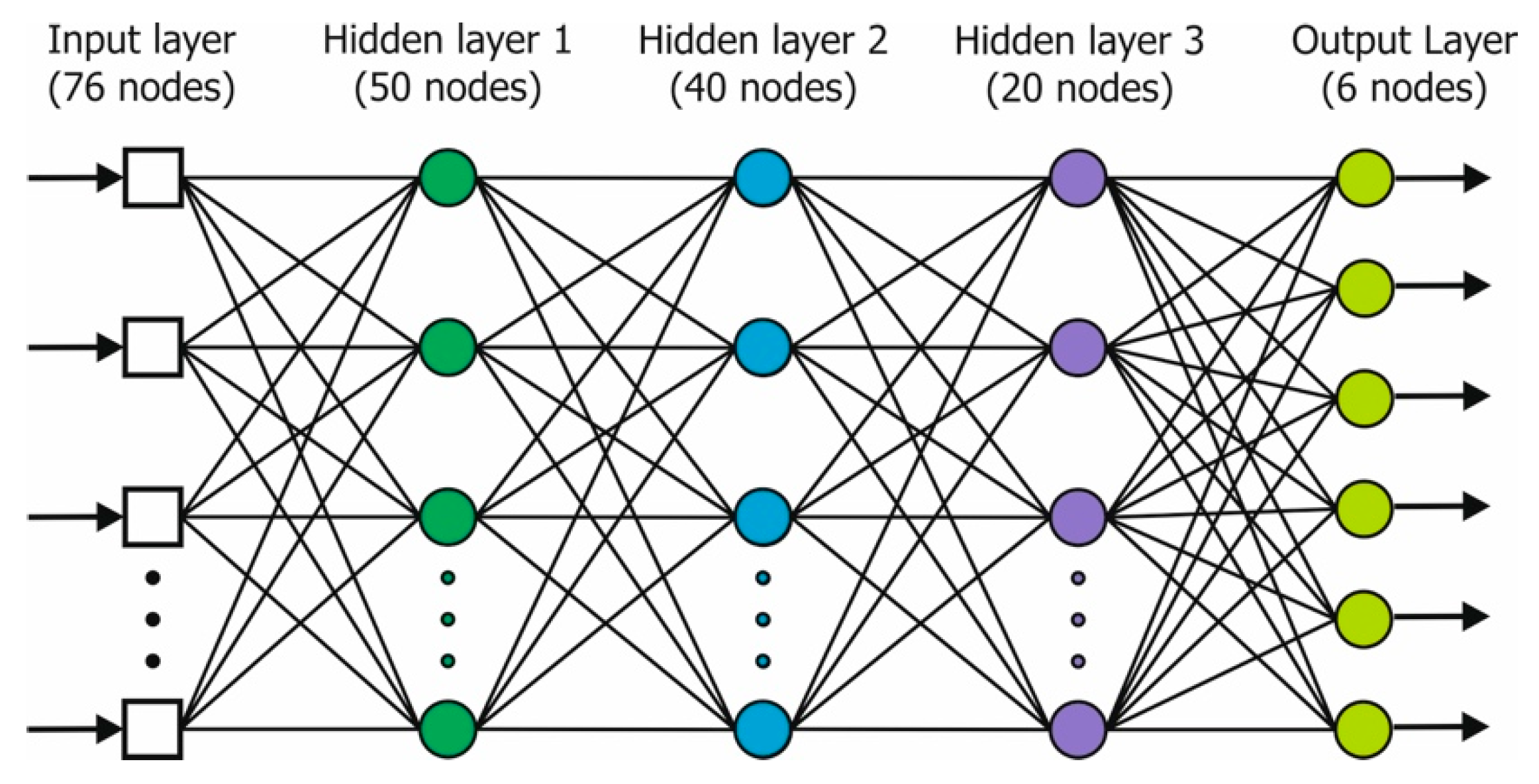
In the course of this research, other less progressive network topologies between input and output for 3H networks were tested, and the results were no better. For this reason, it was decided to use the 3H configuration (76-50-40-20-6) (Figure 8) as a sufficiently good network topology for the problem of the identification of tire parameters. Taking into account that the ANN has a weight to be determined for each connection and that the connections were configured only between adjacent layers, the number of weights to be learned by the ANN can be calculated (76 × 50 + 50 × 40 + 40 × 20 + 20 × 6 = 6720 weights).

Once the ANN configuration is defined and the training dataset is available, the training can start. Figure 9 shows the details of the activities that are executed in this Step 6. In this case, due to the massive input data chosen (100k curves) for the training, the time to complete it was in the range of a full week with an Intel i5 processor. It is important to emphasize that the objective is to have a tool that can give a precise estimate of the parameters of the tire curve from the inputs provided in a universal way (within the range of parameters defined in Table 1). For this reason, the training time of the ANN is not key, since it will be a one-time calculation. Once the network is trained (Step 8), the ANN can be used as an estimation tool that takes only a few milliseconds for the prediction.

It is usually common to divide the number of available curves to train the network into two subsets. The first is used to train the network (training dataset) and the second is a test dataset. The test dataset is not known by the network since their curves have not been used for its training. The performance of the training (Step 7) can be checked in different ways. For example, in Figure 5 the total RMS Error was calculated at eight different epochs. 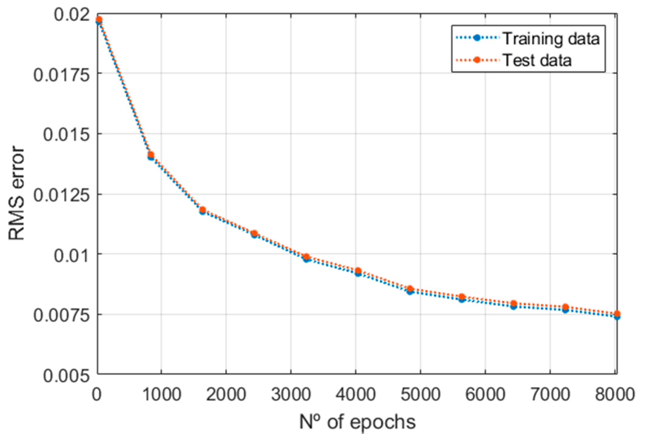Figure 10 shows the RMS Error for both the training and testing datasets, which have a continuously decreasing slope. This indicates that no overtraining has been produced on the ANN and that its prediction capabilities could still be improved providing the training algorithm is run longer. After this process, the ANN has been trained (Step 8) and it can be used for prediction.

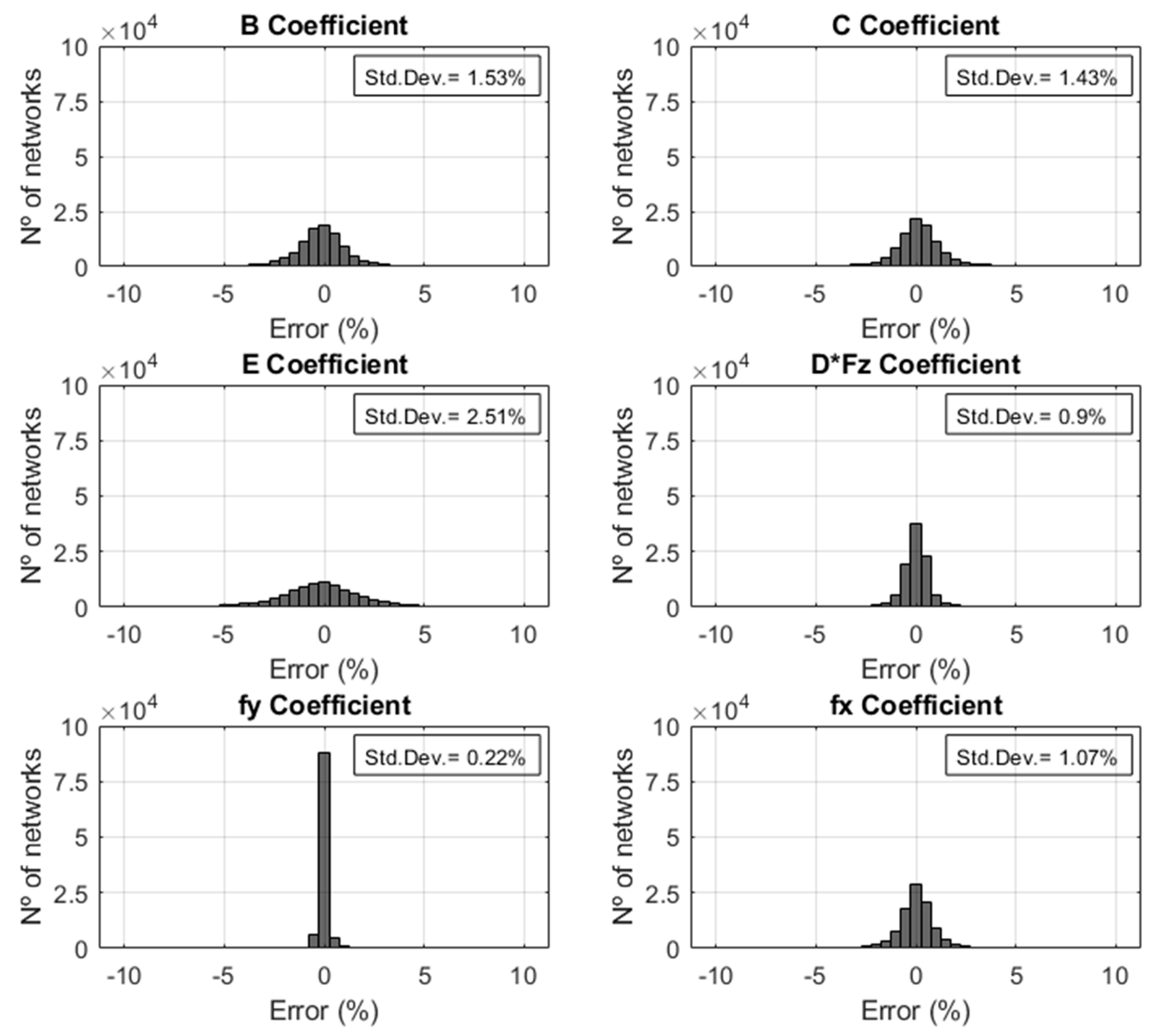
In Figure 11, the prediction error frequencies for the 100k validation curves are shown for the different MF parameters, along with the error standard deviation. Additionally,

Table 2. Range of values for MF model parameters.

Error Range	B (%)	C (%)	E (%)	D*Fz (%)	fy (%)	fx (%)
<5%	98.67	98.81	94.78	99.61	99.99	99.64
5–10%	1.25	1.13	4.71	0.37	0.01	0.35
10–15%	0.06	0.06	0.42	0.02	0	0.01
15–20%	0.02	0.01	0.06	0	0	0
>20%	0	0	0.02	0	0	0

classifies the errors frequencies in classes at every 5%.

It is clearly noticed that a fairly good performance of the network, where the vast majority of the population (over 98%) can be predicted with and error less than 5%, even for D*Fz, fy, and fx parameters, no error data above this value was registered over the complete validation. The most difficult parameter to be predicted is the parameter E, but even in this case, the ANN manages to estimate correctly over 94% of the curves, which can be considered very satisfactory.

3.3. Ann Validation vs. Real Test Data

In the previous section, ANN predictions were validated through “clean” prefabricated data, unknown to the ANN. In this section, we want to take an additional step and analyze the response of the same network when predicting the parameters of real curves obtained in bench tire tests (with different types of errors). The results obtained will serve to draw conclusions about the validity of this methodology against the real problem of identification of parameters of curves from tests (Steps 9 and 10, in Figure 2).

For this purpose, 21 curves from tests measuring the longitudinal force for a 206/65 R15 tire have been used. The curves include seven different slip angles (−8°, −4°, −2°, 0°, 2°, 4° and 8°) in three different normal load (F_z) conditions (2, 3 and 4kN) with a camber of 0. These curves, coming from real tests, have different types of unknown errors. To begin with, the measurement errors are present due to the limited accuracy of the measurement equipment, with their intrinsic uncertainty. On the other hand, it is necessary to take into account the application of slip in steps of 1% between measure and measure, whose uncertainty is not available. In addition, errors and uncertainties can be found regarding the initial condition of the tire or the wear the tire had due to the previous tests or to the roughness of the surface on which the tire runs. Additionally, even environmental variables such as ambient temperature, humidity or wet rolling surface can influence the result of bench acquisitions.

The values of these curves are discretized in the same way as the synthetic curves created in the previous sections so that the ANN can use them directly as input data. In this way, the ANN can give a prediction (Step 9) of the appropriate parameters according to its previous training. As an example, Figure 12 shows the actual data (in dotted red circles) of one of those 21 real curves. The black-discontinued line represents the curve predicted by the ANN.

It is important to be able to evaluate the effectiveness of the prediction of Pacjeka’s parameters by the ANN. For this reason, it is necessary to compare the results of the ANN with other methods. As seen in the state of the art in the introduction, the identification of parameters can be done through many methods (least squares adjustment, genetic algorithms, particle-swarm optimization, etc.). In this case, for the validation, one of the most effective methods has been used, which, although it is not the fastest in the identification of parameters, it is certainly robust: the least squares adjustment [20]. The method has been applied individually to each of the actual tire test curves. In this sense, in Figure 12, the optimal curve, obtained from a non-linear least squares fitting adjustment using the ANN parameters as starting parameters, is drawn in a blue line. It can be seen that the ANN curve (in black) is quite close to the test data and that the optimal curve (in blue), obtained from this through successive iterations, gets an even better fit to the test data (in red).

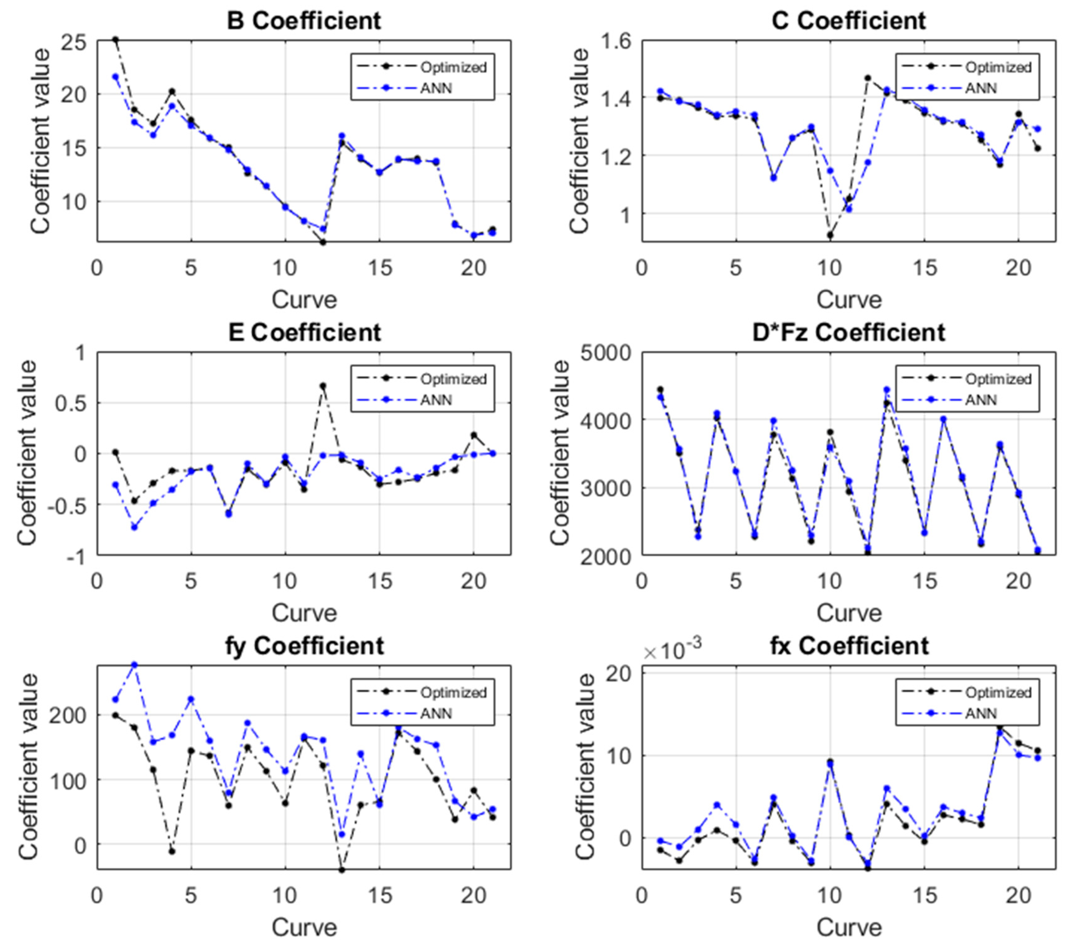
In order to quantify the accuracy of the ANN prediction, a comparison has been made between the parameters obtained from the ANN and those obtained from the optimum curves after a subsequent non-linear curve fitting least squares optimization. The results are shown in Figure 13 and

Table 3. Range of values for MF model parameters.

Error Range	B (%)	C (%)	E (%)	D*Fz (%)	fy (%)	fx (%)
<5%	85.71	90.48	85.71	100	42.86	90.48
5–10%	9.52	0	9.52	0	38.10	9.52
10–15%	4.76	4.76	0	0	9.52	0
15–20%	0	4.76	4.76	0	4.76	0
>20%	0	0	0	0	4.76	0

. From the observation of Figure 13, it is noticed that there is a very good match for B, D·F_z and f_x parameters. C and E also show a high similarity in general, but some isolated predictions with higher differences were also observed. It seems that the most difficult parameter to predict in this case corresponds to f_y.

The ANN, for an error prediction range below 5%, is able to identify correctly more than 85% of the test curves for the parameters B, C, E, D·F_z and f_x. The parameter f_y identifies in that range up to 42.86% of the curves. If the prediction error range is allowed in 10%, then the f_y parameter identifies correctly 81% of the curves. On the other hand, the parameter D·F_z is predicted adequately in 100% of cases.

Therefore, it can be concluded that prediction of the real parameters of the real test bench curves is, for most of the parameters, quite good, as the success percentage is over 85% of the cases. It should be noted however that the f_y parameter can only be predicted within the 5% range only in 42.86% of the cases.

Besides, it should be noted that in all the 21 real cases it was possible to carry out the optimum adjustment of the curves using as initial iteration parameters the ones provided by the ANN prediction (Step 10). Therefore, it seems clear that the results predicted by the ANN, despite errors in the input data, can be used, at least as initial iteration parameters for finer posterior curve fitting if needed.

4. Conclusions

This paper has presented a methodology that allows the creation of an ANN that is able to predict with a high precision the optimum parameters of the basic Pacejka’s Magic Formula when sufficient input data is provided for the training. This ANN can be used as a virtual brain that allows predicting these parameters as long as they are within the range that was used for their training.

In this study, we managed to train an ANN to predict these parameters from perfect mathematical curves obtained from the random variation of the Pacejka’s MF curve parameters. The range of these parameters has been broad enough to cover true values in actual tire curves. The training performed allows for prediction ratios in synthetic curves above 94% for all parameters.

The ANN trained with these mathematical curves has also been used to predict the optimal parameters of real curves obtained in test benches. In this case, the prediction for the majority of parameters is good, obtaining a prediction, within an error range of 5%, of more than 85%. The parameter f_y is the most difficult parameter to predict since only 42.86% of the curves can be predicted within a 5% error range. If the error threshold is raised to 10% then the ANN adequately predicts the f_y parameter for the 80% of the curves.

From the results obtained, the errors identified in the evaluation of curves from real data are limited and, most of the time, very precise. This fact is remarkable if we consider that the ANN was trained for a synthetic data set (with no more error than the Pacejka’s model could have in front of reality), and without having previous information or training of real data coming from tire tests in test benches or from direct interaction data in road tire vehicles.

In addition, once the ANN is pre-trained, it can be applied to any tire or operating condition that falls within the training limits of that ANN. Therefore, it can faithfully represent the operating conditions of a tire by immediately identifying the key parameters of Pacejka’s MF. The computation time is minimal, making it possible to integrate it into more advanced vehicle models. Furthermore, if the ANN is further combined with a real-time dynamic or HIL (hardware in the loop) systems, providing directly acquired tire data on tire-road interaction, a complete adaptive tire model could be achieved, adapted to each of the four wheels separately and to the individual operating or environmental conditions on each of them. This use is left to future research work.

In conclusion, the trained ANN can be used as a standalone reliable identifier of the parameters of a tire curve or as a convenient initial iteration point generator for further refinement.