Abstract
Stroke is considered as a major cause of death and neurological disorders commonly associated with elderly people. Electrocardiogram (ECG) signals are used as a powerful tool in diagnosing stroke, and the analysis of ECG signals has become the focus of stroke research. ECG changes and autonomic dysfunction are reportedly seen in patients with stroke. This study aimed to analyze the ECG features and develop a classification model with highly ranked ECG features as input variables based on machine-learning techniques for diagnosing stroke disease. The study included 52 stroke patients (mean age 72.7 years, 63% male) and 80 control subjects (mean age 75.5 years, 39% male) for a total of 132 elderly subjects. Resting ECG signals in the lying down position are measured using the BIOPAC MP150 system. The ECG signals are denoised using the discrete wavelet transform (DWT) method, and the features such as heart rate variability (HRV), indices of time and spectral domains and statistical and impulsive metrics, in addition to fiducial features, are extracted and analyzed. Our results showed that the values of the HRV variables were lower in the stroke group, revealing autonomic dysfunction in stroke patients. A statistically significant difference was observed in low-frequency (LF)/high-frequency (HF), time interval measured after the S wave to the beginning of the T wave (ST) and time interval measured from the beginning of the Q wave to the end of the T wave (QT) (p < 0.05) between the groups. Our study also highlighted some of the risk factors of stroke, such as age, male sex and dyslipidemia (p < 0.05), that are statistically significant. The k-nearest neighbors (KNN) model showed the highest classification results (accuracy 96.6%, precision 94.3%, recall 99.1% and F1-score 96.6%) than the random forest, support vector machine (SVM), Naïve Bayes and logistic regression models. Thus, our study reported some of the notable ECG changes in the study participants and also indicated that ECG could aid in diagnosing stroke disease.
Keywords:
stroke; risk factors; ECG; heart rate variability; classification; machine learning models 1. Introduction
One of the major diseases associated with the elderly is a stroke and is considered as the second leading cause of death with the third most common cause of disability-adjusted life years (DALYs) [1,2]. Stroke is a medical emergency condition, and prompt treatment is crucial also; earlier action can reduce brain damage and other complications. The risk of stroke increases significantly for elderly adults [3,4]. According to the World Health Organization (WHO), by 2050, the world’s population of those aged 60 years and beyond is projected to reach two billion, up from 900 million in 2015. In Korea, stroke is a major health burden that will substantially increase in the near future, and Korea is becoming the most rapidly aging society in the world [5]. A study based on the stroke incidence rate of some countries reported that 75–89% of strokes occur in individuals aged >65 years; of those, 50% occur in people aged ≥70 years and 25% in those who are aged >85 years [6]. As of 2013, the global mortality and disability rate caused by stroke were nearly 6.5 million and 113 million, respectively, whereas the mortality rate is higher in Asia than in Europe and the Americas [7]. Another study reported that the stroke mortality rate of Korea sharply increased, particularly after the age of 70 years [2]. Approximately, every year, 105,000 people experience a new or recurrent stroke, and more than 26,000 people die due to stroke, which indicates that, every five min, a stroke attacks someone, and in every 20 min, a stroke kills someone in Korea. This results in a substantial economic burden to Korea, with the total nationwide cost for stroke care nearly 3.3 billion US dollars in 2005 [1]. The duration of hospital stay and medical expenditure is higher in stroke patients than patients with other chronic diseases [8]. Therefore, an early diagnosis of stroke can enable us to save the lives of people, and the research on stroke patients is also very important for the effective utilization of medical resources.
Conventionally, stroke has been diagnosed by various methods, such as computed tomography (CT), magnetic resonance imaging (MRI), a blood test and electrocardiogram (ECG) signals. ECG has always been considered as a popular measurement scheme that is comparatively low-cost in screening and diagnosing various diseases [9]. It has a variety of applications in health monitoring and auxiliary diagnosis and plays a valuable complementary technique for stroke diagnostics [10]. ECG has been mainly used for stroke detection, which helps to determine the cause of stroke. Since the investigation of ECG signals is noninvasive by placing the electrodes on the skin, this helps in the accurate detection of abnormalities. Therefore, a baseline ECG can be useful for detecting cardiac abnormalities in acute stroke patients [11].
In medicine, machine learning has great hope in predicting the disease and assisting doctors in diagnosis, using data collected by wearable sensors and smartphones. The use-case of the machine-learning model is both a diagnosis or prognosis in which the diagnostic models can be used for new subjects, and the model developed for prognosis can predict a given subject’s future clinical state [12]. The machine-learning and deep-learning techniques such as logistic regression, random forest and deep neural networks are used for predicting the presence of stroke disease with various related attributes [13,14]. The stroke risk classification techniques are developed by using logistic regression, Naïve Bayesian, Bayesian network, decision tree, neural network, random forest, bagged decision tree, voting and boosting models [15]. Additionally, the machine-learning algorithms are capable of identifying the features that are highly related to stroke occurrence efficiently from the huge set of features [16].
Several studies focused on patient classification based on the overall behavior of the ECG to diagnose specific diseases [17]. The extraction of features from the ECG signal is a key step for ECG recognition, as it allows to greatly enhance and extract the characteristics of the signal, and those features can be fed into the conventional machine-learning models to perform the classification [18]. The integration of classification techniques in the clinical setup majorly requires the detection of ECG abnormalities in real time to be used in the hospital environment at the bedside or on wearable devices [17]. In general, ECG abnormalities are frequently seen in patients with a stroke. A study revealed that any ECG abnormality is a highly ranked factor, and it may be possible that all ECG abnormalities are more indicative of stroke than just atrial fibrillation [16]. Therefore, the analysis of ECG features and the detection of abnormalities from the ECG signal are significant tasks for the diagnosis of stroke disease. With the consideration of the importance of ECG changes in stroke [19], our study aimed to analyze the ECG features for the classification of elderly post-stroke patients and control subjects with a stroke diagnostic approach. Firstly, we extracted the features from the denoised ECG signals of the study participants. Secondly, we performed the analyses on the features such as heart rate variability (HRV) indices of time and spectral domains, fiducial features and statistical and impulsive metrics variables that have not been commonly used. Thirdly, we employed the filter-based feature selection approach for selecting the input feature subset for the classifiers. Finally, we intended to develop a classification model for diagnosing stroke disease based on machine-learning techniques such as k-nearest neighbor (KNN), support vector machine (SVM), Naïve Bayes, random forest and logistic regression. Furthermore, our study aimed to investigate the autonomic dysfunction and the potential risk factors in relation to stroke.
2. Materials and Methods
2.1. Study Participants and Data Collection
A total of 132 participants, including 52 stroke patients with the mean age of 72.7 (SD 6.6) and 80 control subjects with the mean age of 75.5 (SD 3.4), were recruited for this study. The stroke subjects who participated in this study were the outpatient volunteers diagnosed with stroke within one year at the time of data collection capable of independent walking and using assistance tools. The control subjects are those without physical or cognitive impairments caused by cerebrovascular disease such as stroke. The subjects with an acute or chronic infections such as liver failure, renal failure and cancer were excluded in this study. The ECG signals were measured using the BIOPAC MP150 (BIOPAC Systems Inc., Goleta, CA, USA) with the standard three lead measurements, conducted in Chungnam National Hospital, Daejeon, South Korea from 2017 to 2018. Resting ECG signals were obtained for a period of 5 min in the lying down position. The blood samples from the study participants were taken after overnight fasting before ECG recordings. All the clinical parameters were determined in the laboratory of Chungnam National Hospital. The demographics and clinical data such as age, gender, body mass index (BMI), systolic blood pressure (SBP), diastolic blood pressure (DBP), hemoglobin, low-density lipoprotein (LDL), high-density lipoprotein (HDL), total cholesterol and cardiovascular risk factors such as hypertension and dyslipidemia were included in this study. Hypertension was assessed with the repeated measures of systolic blood pressure ≥140 mmHg or diastolic blood pressure ≥90 mmHg, and diabetes was assessed with the blood glucose level ≥126 mg/dL. A family history of stroke was evaluated if one or both of the parents of the subjects had a stroke. Smoking was determined as having smoked at least once per day or more for one year and reported current smoking. Alcohol consumption was classified as current drinkers who drink on a daily or weekly basis at least once per week at present. Smoking and alcohol levels were assessed using a questionnaire, and the National Institute of Health Stroke Scale (NIHSS) was used to evaluate the stroke severity of the patients. The individual scores of each feature are summed to calculate the total NIHSS score. The maximum severity score is 42, and the minimum is 0. In a total of 52 stroke patients, there were 8 patients with minor stroke (NIHSS: 1–4), 12 patients with moderate stroke (NIHSS: 5–15), 13 patients with moderate-to-severe stroke (NIHSS: 16–20) and 19 patients with severe stroke (NIHSS: 21–42).
2.2. Data Analysis
Statistical analysis was executed in IBM SPSS 23.0 Software (SPSS Inc., Chicago, IL, USA), and the categorical variables were represented as frequency and percentage, whereas the continuous variables were presented as mean and standard deviation. The comparison between the quantitative measurements was performed using the independent t-test. The chi-square test was implemented to evaluate the differences between categorical variables. The one-way analysis of variance (ANOVA), followed by Tukey’s test, was used to compare the groups on possible differences in HRV indices, impulsive metrics and ECG intervals. A p-value < 0.05 was considered as statistically significant. The Pearson correlation analysis was performed to find the multicollinearity. We computed a boxplot to represent the distribution of the values for the features, with significant differences. The simulations such as signal denoising and classifications using machine-learning models were performed in MATLAB R2020a (The Mathworks Inc., Natick, MA, USA).
2.3. ECG Signal Denoising Based on Discrete Wavelet Transform Method
ECG signals are often accompanied by noise and interference. Therefore, the denoising of ECG signals is necessary before performing the feature extraction. Wavelet analysis helps to remove the noises and improves the signal strength [20]. The discrete wavelet transform (DWT) is a widely used method to decompose the signal simultaneously into time and frequency domain information. In general, to denoise the signal using DWT, we need to decompose the signal into L levels and select the suitable mother wavelet function [21]. The types of mother wavelets are Daubechies, Haar, Symlets, Biorthogonal, Coiflets, etc. However, selecting a relevant wavelet is the most important task, as there is no universal method to choose a particular wavelet. The wavelets are derived from a single prototype wavelet y(t) called the mother wavelet by scaling and shifting the parameters, as expressed in [21] Equation (1).
where a represents the scaling factor, and b represents the shifting factors.
Daubechies wavelet is one of the most perspective discrete wavelets transforms, with the basic properties of orthogonality, normalization and compactness of support [22]. The process of signal denoising based on discrete wavelet transform consists of decomposition of the signal, thresholding and reconstruction of the signal [23]. In the hard thresholding method, the wavelet coefficients with absolute values below or at the threshold level are replaced by zero, and the others are kept unchanged. In the soft threshold, when the absolute value of the wavelet coefficient is less than the given threshold value, set it as zero. If the coefficient is larger than the given threshold value, let the wavelet coefficient subtract the threshold value [24].
Soft thresholding provides smoother results than the hard thresholding method [25]. We used the Daubechies as the mother wavelet of order eight and decomposed the signals into four levels using a soft thresholding technique. The Daubechies wavelet of order 8 (db8) of the original and denoised ECG signal is shown in Figure 1.
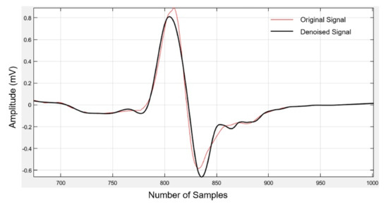
Figure 1.
Original and denoised electrocardiogram (ECG) signal using Daubechies wavelet transform.
2.4. Feature Extraction
In this step, a total of 21 features, including the HRV time and spectral domain variables, intervals between the fiducial points and higher-order statistical and impulsive metric variables are extracted.
2.4.1. Statistical Time-Domain Features
- Kurtosis—Calculates whether the data is heavy-tailed or light-tailed relative to a normal distribution.
- Skewness—Computes the asymmetry of the data. When the data points are skewed to the left, it is called a negative skew, and data points skewed to the right are called a positive skew.
- Peak value—Gives the maximum absolute value of the signal.
- Impulse factor—Compares the height of a peak to the mean level of the signal.
- Crest factor—Defined as the peak value divided by the root mean square value.
2.4.2. Time Domain Variables of Heart Rate Variability (HRV)
The heart rate variability indices of the time domain are calculated and are expressed [26] in Equations (2)–(4).
RMSSD—Computed as the root mean square of the sum of the squares of differences between adjacent RR intervals (RR-I) in milliseconds.
SDSD—The standard deviation of adjacent RR-I differences measured in the units of milliseconds.
pNN50—The percentage of intervals greater than 50 ms different from the proceeding interval.
2.4.3. Frequency Domain Variables of HRV
The frequency domain variables are used to discriminate the sympathetic and parasympathetic activity of RR-I. The spectral power in the low-frequency (LF) band (0.04–015 Hz) is related to the sympathetic-parasympathetic activity. On the other hand, the high-frequency (HF) band (0.15–0.4 Hz) is associated with the parasympathetic activity [27]. The range of spectral power in the very low-frequency (VLF) band is 0.003–0.04 Hz. In this work, the VLF, LF, HF and ratio of LF and HF (LF/HF) band power spectral densities are evaluated as the frequency domain features.
2.4.4. Fiducial Features
The ECG abnormalities can be detected using the features of the ECG signal, and it comprises the P-wave, time interval of the QRS complex (QRS) and T-wave, which includes the corresponding onset, offset and peak points and are represented as fiducial points, as shown in Figure 2 [28]. The features of an ECG signal are nothing but the segments and intervals between the fiducial points [29]. In this experiment, the fiducial points are detected based on the the Pan-Tompkins QRS detector and the corresponding intervals, such as RR-I (ms), heart rate (bpm), QRS complex (ms), time interval measured from the beginning of the P wave to the peak of the R wave (PRQ) in ms, amplitude of the R wave (R-H) in mV, amplitude of the P wave (P-H) in mV, time interval measured after the S wave to the beginning of the T wave (ST) in ms, time interval measured from the beginning of the Q wave to the end of the T wave (QT) in ms and corrected QT interval (QTc) in ms from the ECG signals extracted using BIOPAC Acqknowledge 5.0 software (BIOPAC systems Inc., Goleta, CA, USA).
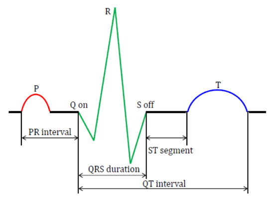
Figure 2.
Fiducial points and features of the ECG signal. PR: time interval measured from the beginning of the P wave to the start of the QRS complex, QRS: time interval of the QRS complex, ST: time interval measured after the S wave to the beginning of the T wave and QT: time interval measured from beginning of the Q wave to the end of the T wave.
2.5. Feature Selection and Ranking
Feature selection approaches reduce the dimensionality of data by choosing a subset of predictor variables. It also enables the machine-learning algorithms to train faster and improves the accuracy of the model with the selection of the right subset. The feature selection techniques are further classified into the filter, wrapper and embedded methods [30]. The main challenge is the redundancy of the features, and the existing dimensionality reduction technique such as principal component analysis (PCA) is not suitable to build the applicable and human understandable models [31]. The filter-based feature selection approaches are investigated and found to be effective in selecting the features that are associated with stroke [32]. In this research, we applied one of the filter-based feature selection approaches, such as ANOVA, to select the optimal feature subset. The computational speed of the filter methods are much faster than the wrapper methods. ANOVA is a statistical test useful in comparing two or more mean values. For each feature, if the p-value is near to 0, there exists significant differences in the characteristic values for the different categories [33]. Feature importance ranking from the results of the ANOVA F-test are shown in Figure 3. Features that did not achieve sufficient significance (p ≥ 0.05) are omitted. Therefore, we selected three features such as LF/HF, ST and QT that showed statistical significance (p < 0.05) and are the highly ranked features. The correlation analysis was then performed to find the relation between these three features. The correlation coefficient r = −0.16 between LF/HF and QT indicates a weak negative correlation and reveals the inverse relationship between LF/HF and QT. Similarly, the correlation coefficient r = −0.19 between LF/HF and ST represents a weak negative correlation. Further, the ST and QT intervals indicate a moderate positive correlation of r = 0.44. As there are no strong correlations between these features, we selected LF/HF, ST and QT as the input features subset for the classification models.
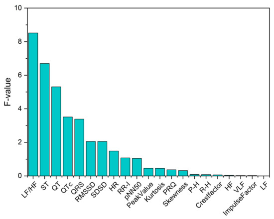
Figure 3.
Ranking of overall features based on the ANOVA F-test. LF: low-frequency, HF: high-frequency, QTc: corrected QT interval, RMSSD: root mean square of the sum of the squares of differences between adjacent RR intervals, SDSD: standard deviation of adjacent RR intervals differences, HR: heart rate, RR-I: RR intervals, pNN50: percentage of intervals greater than 50 ms different from the proceeding interval, PRQ: time interval measured from the beginning of the P wave to the peak of the R wave, P-H: amplitude of P wave, R-H: amplitude of R wave and VLF: very-low-frequency.
2.6. Machine-Learning Classification Approach
We applied the SVM, KNN, Naïve Bayes, random forest and logistic regression models in our classification approach. The SVM classifies data by finding the best hyperplane that separates all data points of one class from the other class, and it is widely used in pattern recognition, image processing and classification [18]. KNN stores all cases and classifies the new cases based on similarity measures [34]. The Naïve Bayes classifier is based on the Bayes theorem, and it is characterized by high accuracy and scalability, even for a very large volume of data [35]. The logistic regression is mainly used to predict the outcome of a categorical dependent variable from a set of predictor variables [36], and the random forest technique is also widely used in stroke prediction [13]. We performed the model validation process for evaluating a trained model on the test dataset. In particular, an overfitting problem occurs by fixing a training set and a test set when generating a predictive model [37]. Therefore, in this study, the classification performance is measured by constructing a training set and a test set with 10-fold cross-validation method.
3. Results
3.1. Baseline Clinical Characteristics
The demographics, hemodynamic and clinical data of the study population are presented in Table 1. Among the overall study population, the stroke group had a mean age of 72.7 ± 6.6 years, with 33 (63%) men, while the control group mean age was 75.5 ± 3.4 years, with 31 (39%) men. The stroke subjects were moderately younger than the control subjects (p < 0.05). In subjects with stroke, the components were distributed as follows: Subjects who have drinking practice were 12 (23%), and a smoking habit was noticed in 16 (31%) and hypertension in 18 (35%), whereas diabetes was present in 8 (51%), whilst the subjects diagnosed with heart diseases were 3 (6%) in the stroke group. There was no significant difference observed in the BMI values between the groups. However, a significant difference between the stroke and control groups was noticed with respect to age, male sex and dyslipidemia, with a p-value < 0.05. Furthermore, the family history of stroke was identified as five (10%) for the stroke group and five (6%) for the controls. The baseline NIHSS for the stroke subjects was shown in the median (interquartile range, IQR) as 25 (6). The clinical assessment showed that there was no significant difference in systolic, as well as in diastolic, blood pressure between the groups. The hemoglobin levels were found to be similar between the groups. Further, the HDL level was higher in the stroke group, whereas the LDL and total cholesterol levels were found to be lower in the stroke subjects than the controls.

Table 1.
Demographics and clinical data of the stroke and control groups.
3.2. HRV Analysis of Stroke and Control Group
There was no significant difference in the RMSSD values between the strokes and controls. However, the analysis of calculating the variability of the adjacent RR-I values revealed that the RMSSD index was reliably lower in the stroke group, whereas the SDSD did not differ significantly. A similar trend was observed in the pNN50 index, which gives the proportion of NN50 divided by the total number of RR-I summarized in Table 2. From the frequency domain analysis, the RR-I variability in the VLF bandwidth shows no significant difference between the groups. In the HF and LF bandwidths, a downward trend was observed in the stroke group. A significant difference was evident in the LF/HF ratio, also called the sympathovagal balance (F = 8.21, p = 0.014). The post hoc comparisons using Tukey’s honestly significant difference (HSD) test indicated that the mean score for the stroke group (1.18 ± 0.21) was significantly different than the control group (0.60 ± 0.079), and the boxplot shown in Figure 4 represents the distribution of the LF/HF values. This analysis of the time and frequency domain variables indicated that subjects with a stroke showed a decrease in the heart rate variability.
Table 2.
Time and frequency domain indices of the heart rate variability (HRV).
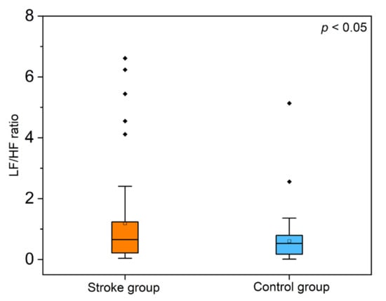
Figure 4.
Boxplot representation of the low-frequency/high-frequency (LF/HF) ratio from the heart rate variability (HRV) spectral domain analysis (p < 0.05 between the groups).
3.3. Analysis of Higher Order Statistics and Impulsive Metrics Variables
The statistical metrics such as kurtosis and skew were slightly higher in the stroke group, with no significant differences (p > 0.05). The peak value was slightly lower in the subjects with strokes, 1.05 ± 0.37 vs. 1.10 ± 0.47 in the controls. The impulsive metrics analysis revealed that the impulse factor was higher, whereas the crest factor was lower in the stroke group given in Table 3. Figure 5 illustrates the mean and standard deviation values of the variables between the groups.
Table 3.
Higher order statistical and impulsive metrics of the stroke and control groups.
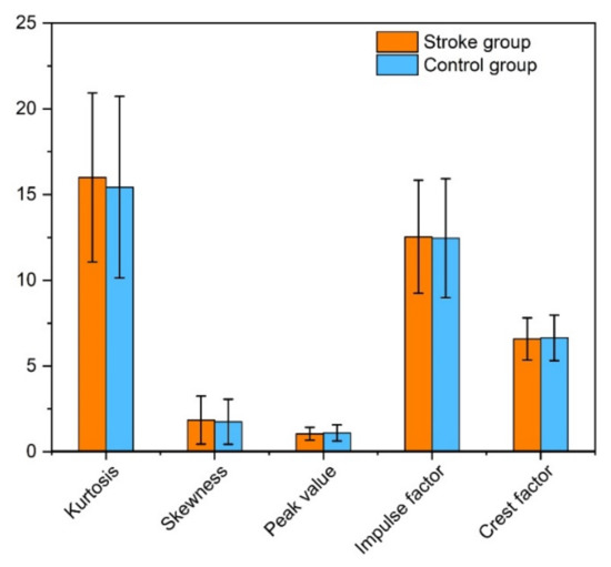
Figure 5.
Bar graph illustration of the mean and standard deviation values of the statistical and impulsive metric variables of the stroke and control groups.
3.4. Analysis of Intervals Extracted between the Fiducial Points of ECG
The extracted intervals of the stroke and control groups between the fiducial points of the ECG are represented in Table 4. The RR-I value represents the time between the QRS complexes that was noted to be lower in the stroke subjects than the control group (890 ± 140 ms vs. 920 ± 130 ms) and exhibits no significant difference (p > 0.05). Consequently, the heart rates were 68.87 ± 11.7 bpm for the stroke subjects, while the control group were 66.51 ± 9.89 bpm. The PRQ, which is the time interval measured from the beginning of the P wave to the peak of the R wave, appeared slightly lower among the subjects with strokes than the control subjects (179 ± 26 ms vs. 182 ± 28 ms, p > 0.05). The time interval of the QRS complex between the two groups showed no significant results, but an increasing trend was noticed among the stroke subjects.
Table 4.
Fiducial features of the electrocardiogram (ECG).
The results revealed that the amplitude of the P wave (P-H) appeared slightly lower among the stroke group, whereas the R wave amplitude (R-H) was more pronounced in the stroke group. Furthermore, the QT interval measured from the start of the Q wave to the end of the T wave was statistically significant (F = 5.30, p = 0.029), followed by the Tukey’s test, which represented the mean score for the stroke group (512 ± 56) and was significantly different than the control group (533 ± 46). Although, the corrected QT interval (QTc) showed a downward trend similar to the QT interval, with no statistically significant results. Additionally, the time interval measured after the S wave to the beginning of the T wave, called the ST interval, showed significance (F = 6.70, p = 0.014), and the Tukey’s test indicated that the mean score of the stroke subjects (427 ± 59) was more statistically significant than the control subjects (452 ± 49). To summarize from the results, the QT and ST are the two intervals that showed a significant difference between the two groups illustrated as boxplot graphs in Figure 6.
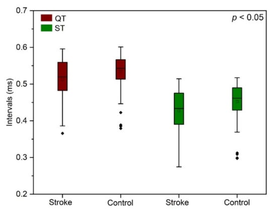
Figure 6.
Boxplot illustration of the distribution of QT (p = 0.029) and ST intervals (p = 0.014) between the stroke and the control subjects.
3.5. Classification Model
In this experiment, we used the logistic regression, random forest, Naïve Bayes, SVM and KNN algorithms to perform the classification, and the features fed into the classifiers were the LF/HF, ST and QT. We performed the hyperparameter optimization before training the classifier models, as it plays a vital role in the classification accuracy of machine-learning models. The models are evaluated using performance metrics such as accuracy, precision and recall. Accuracy is measured in terms of the number of correctly classified data points out of all the data points. The receiver operating characteristic (ROC) curve is the most effective tool for measuring the accuracy [38]. However, in most of the classification problems, imbalanced class distribution exists, and the F1-score is used to evaluate the model. We used the following parameters: true positive, true negative, false positive and false negative to calculate the performance metrics. True positive represents the correctly classified stroke rate, whereas true negative represents the correctly classified nonstroke rate. The false negative and false positive provide the incorrectly classified nonstroke and stroke rates, respectively. The accuracy, precision, recall and F1-scores were calculated as follows [8]:
Precision = True positive/(True positive + False positive)
Recall = True positive/(True positive + False negative)
F1-score = 2 × ((precision × recall)/(precision + recall))
Accuracy = (True positive + True negative)/(True positive + True negative + False positive + False negative)
Table 5 summarizes the computational results obtained from the classifier models and listing of the four performance parameters. Considering all the models, the highest classification accuracy 96.6%, precision 94.3% and recall 99.1% were acquired by the KNN model, with the F1-score as 96.6%. Thus, the KNN algorithm provided the best performance results, followed by random forest with 94.4% accuracy, 91.7% precision, 97.7% recall and a 94.6% F1-score. Further, the SVM showed the performance results of 85.4% accuracy, 81.5% precision, 91.7% recall and a 86.3% F1-score. The Naïve Bayes algorithm attained 72.7% accuracy, 64.2% precision, 87.8% recall and a 74.1% F1-score, whereas the least performance results were given by the logistic regression model as 66.9% accuracy, 57.1% precision, 91.7% recall and a 70.3% F1-score. The results showed that the KNN classifier model outperformed the other models.
Table 5.
Results of the classification performance of the models.
4. Discussion
In the present study, we highlighted the major risk factors of stroke obtained from the statistical analysis of the baseline demographics and clinical characteristics of the study population. We demonstrated the use of a machine-learning algorithms and developed a classification model with highly ranked ECG features obtained from various datasets, such as the HRV parameters of the time and spectral domains, statistical and impulsive metric variables and ECG intervals.
Christian Tanislav et al. reported the higher mean age and overrepresentation of male sex in the baseline characteristics of stroke patients [39]. In a study conducted by Ginenus Fekadu et al., the number of males found to be higher consisted of 62.9% among the overall stroke patients [40]. Similarly, our findings noticed that the number of male stroke subjects accounted were higher and comprised 63% more than female stroke subjects. Some of the major risk factors for stroke are reported as age, hypertension, diabetes, dyslipidemia, cardiovascular diseases and smoking and alcohol consumption [41]. Our study disclosed the most significant risk factors for stroke as age, gender and dyslipidemia (p < 0.05), and thereby, people with one or more of these risk factors are considered to be at high risk of stroke.
Besides the demographics and clinical data, we explored the HRV indices of time and frequency domains to find the autonomic dysfunction of the stroke subjects. Acute stroke generally affects the autonomic nervous system, and the reduction in HRV is a regular sign of illness in stroke patients [42]. Several studies also reported that a lower heart rate variability was associated with a higher risk of incident stroke [43,44,45,46]. Correspondingly, our results noticed a lowered value of RMSSD, SDSD and pNN50 of the time domain parameters and lowered LF, HF and VLF of the frequency domain parameters for the stroke subjects, indicating the relation of lower heart rate variability with stroke. Furthermore, we observed that the stroke patients had elevated values of the LF/HF ratio, similar to the findings of Tokgozoglu et al. and Colivicchi et al., which revealed that the patients with acute strokes had increased LF/HF values when compared to the normal people [47,48]. However, no significant differences were observed in the higher order statistical and impulsive metric variables between the groups. The prevalence of ECG changes have a significant relationship with aging [49]; additionally, the ECG abnormalities are regularly seen in stroke patients [50,51]. Many studies reported that the most common ECG abnormalities associated with acute stroke are arrhythmia, prolonged QTc and T wave and U wave abnormalities [19,52,53,54,55]. Accordingly, we noticed the prolonged QTc in the stroke group, including both male and female subjects, with the overall mean value of the QTc greater than 450 milliseconds. A similar trend also seen in the control group might because of the aging effects [56]. In addition to that, we identified a slightly prolonged QRS duration, with the mean value of the QRS greater than 110 ms in the stroke group. However, a significant difference was detected only in the QT and ST intervals between the study populations. Thus, our study performed an extensive analysis on the extracted features and also noted significant changes.
Machine-learning techniques belong to the domain of artificial intelligence, and they provide a promising tool in pursuing personalized outcome predictions and globalized diagnostic models, which are increasingly used in medical research [12,13,57,58,59]. The major findings from our work were that LF/HF, ST and QT are the three highest-ranking ECG attributes considered to be the optimal input features subset for classifying an individual as a stroke or control, whereas the rest of the features that did not show significance (p ≥ 0.05) were excluded. Therefore, our study appropriately selected the features for the classifiers. The KNN model outperformed, with a higher classification accuracy than the other models, and the results indicated that our approach can achieve the best performance accuracy using limited attributes that have not been commonly used in the classification models.
This study has some limitations that offer future research opportunities. Our model included only the features of the ECG and excluded the risk factors obtained from the baseline data. This may cause an impact on the overall accuracy of the model. The model needs to be validated using subject-wise cross-validation, as the record-wise cross-validation may overestimate the performance of the model. Additionally, the performance of the proposed model needs to be compared with the existing models. Another limitation is the lack of evidence about the higher-order statistical and impulsive metric variables in relation to stroke. Although our study found significant differences in the ECG intervals, it would be worth conducting a subanalysis to find the prevalence of ECG abnormalities among the stroke population. The present study did not take into consideration the details of the medications for stroke patients. However, the ECG changes may be confounded by stroke medications such as beta-blockers or antiarrhythmic drugs that require further investigation. This is a small-scale study whose findings need to be validated further by including larger population studies.
5. Conclusions
In summary, we analyzed the ECG features of elderly stroke and control subjects to describe the significant changes between the two groups, as ECG signals can be a tool for medical practitioners to detect various abnormalities related to stroke. Further, we investigated autonomic dysfunction in post-stroke patients with the exploration of HRV variables. Additionally, we highlighted the risk factors of stroke obtained from the baseline characteristics of the study participants. The classification model was developed using ECG features based on machine-learning techniques. For diagnosing stroke disease, the KNN model attained the best results in classifying an individual as a stroke patient or control subject using only three features. Thus, the analysis results of the ECG signals indicate that the highly ranked ECG features acquired from our findings might be the suitable key features in identifying stroke, and the proposed model may assist in diagnosing stroke disease based on ECG signals for clinical utility.
Author Contributions
Conceptualization, K.R.; formal analysis, S.J.P.; funding acquisition, S.J.P.; investigation, K.R.; methodology, K.R.; project administration, S.J.P.; software, K.R.; supervision, S.J.P.; validation, K.R. and S.-N.M.; writing—original draft preparation, K.R.; writing—review and editing, K.R.; S.J.P. and S.-N.M. All authors have read and agreed to the published version of the manuscript.
Funding
The work was supported by the National Research Council of Science & Technology (NST) grant by the Korea government (MSIP) (No. CRC-15-05-ETRI).
Institutional Review Board Statement
The study was conducted according to the guidelines of the Declaration of Helsinki and approved by the Institutional Review Board of Korea Research Institute of Standards and Science (KRISS-IRB-2016-05-19).
Informed Consent Statement
Informed consent was obtained from all subjects involved in the study.
Data Availability Statement
The data that support the findings of this study are available upon reasonable request from the corresponding author. The data are not publicly available due to the confidentiality and privacy of the research participants.
Conflicts of Interest
The authors declare no conflict of interest.
References
- Hong, K.S.; Bang, O.Y.; Kang, D.W.; Yu, K.H.; Bae, H.J.; Lee, J.S.; Heo, J.H.; Kwon, S.U.; Oh, C.W.; Lee, B.C.; et al. Stroke statistics in Korea: Part I. epidemiology and risk factors: A report from the Korean stroke society and clinical research center for stroke. J. Stroke 2013, 15, 2–20. [Google Scholar] [CrossRef]
- Kim, J.Y.; Kang, K.; Kang, J.; Koo, J.; Kim, D.H.; Kim, B.J.; Kim, W.J.; Kim, E.G.; Kim, J.G.; Kim, J.M.; et al. Executive summary of stroke statistics in Korea 2018: A report from the epidemiology research council of the korean stroke society. J. Stroke 2019, 21, 42–59. [Google Scholar] [CrossRef]
- Reddy, H.P.; Jaganath, A.; Nagaraj, N.; Reddy, V.Y.J. A study of age as a risk factor in ischemic stroke of elderly. Int. J. Res. Med. Sci. 2019, 7, 1553–1557. [Google Scholar] [CrossRef]
- Olindo, S.; Cabre, P.; Deschamps, R.; Chatot-Henry, C.; Rene-Corail, P.; Fournerie, P.; Saint-Vil, M.; May, F.; Smadja, D. Acute stroke in the very elderly epidemiological features, stroke subtypes, management, and outcome in matinique, french west Indies. Stroke 2003, 34, 1593–1597. [Google Scholar] [CrossRef] [PubMed]
- Choi, S.J. Agening society issues in Korea. Asian Soc. Work Policy Rev. 2009, 3, 63–83. [Google Scholar] [CrossRef]
- Chen, R.L.; Balami, J.S.; Esiri, M.M.; Chen, L.K.; Buchan, A.M. Ischemic stroke in the elderly: An overview of evidence. Nat. Rev. Neurol. 2010, 6, 256–265. [Google Scholar] [CrossRef] [PubMed]
- Venketasubramanian, N.; Yoon, B.W.; Pandian, J.; Navarro, J.C. Stroke epidemiology in south, east and south-east Asia: A review. J. Stroke 2017, 19, 286–294. [Google Scholar] [CrossRef] [PubMed]
- Cheon, S.; Kim, J.; Lim, J. The use of deep leaning to predict stroke patient mortality. Int. J. Environ. Res. Public Health 2019, 16, 1876. [Google Scholar] [CrossRef] [PubMed]
- Serhani, M.A.; Kassabi, T.H.E.; Ismail, H.; Navaz, A.N. ECG monitoring systems: Review, architecture, processes and key challenges. Sensor 2020, 20, 1796. [Google Scholar] [CrossRef]
- Xie, Y.; Yang, H.; Yuan, X.; He, Q.; Zhang, R.; Zhu, Q.; Chu, Z.; Yang, C.; Qin, P.; Yan, C. Stroke prediction from electrocardiograms by deep neural network. Multimed. Tools Appl. 2020. [Google Scholar] [CrossRef]
- Adeoye, A.M.; Ogah, O.S.; Ovbiagele, B.; Akinyemi, R.; Shidali, V.; Agyekum, F. Prevalence and prognostic features of ECG abnormalities in acute stroke: Findings from the SIREN study among africans. Global Heart 2017, 12, 99–105. [Google Scholar] [CrossRef]
- Saeb, S.; Lonini, L.; Jayaraman, A.; Mohr, D.C.; Kording, K.P. The need to approximate the use-case in clinical machine learning. Gigasicence 2017, 6, 1–9. [Google Scholar] [CrossRef] [PubMed]
- Heo, J.N.; Yoon, J.G.; Park, H.; Kim, Y.D.; Nam, H.S.; Heo, J.H. Machine learning–based model for prediction of outcomes in acute stroke. Stroke 2019, 50, 1263–1265. [Google Scholar] [CrossRef] [PubMed]
- Chantamit-o-pas, P.; Goyal, M. Prediction of Stroke Using Deep Learning Model. In Neural Information Processing. ICONIP 2017. Lecture Notes in Computer Science; Liu, D., Xie, S., Li, Y., Zhao, D., El-Alfy, E.S., Eds.; Springer: Cham, Switzerland, 2017; Volume 10638, pp. 774–781. [Google Scholar]
- Li, X.; Bian, D.; Yu, J.; Li, M.; Zhao, D. Using machine learning models to improve stroke risk level classification methods of China national stroke screening. BMC Med. Inform. Decis. Mak. 2019, 19, 261. [Google Scholar] [CrossRef] [PubMed]
- Khosla, A.; Cao, Y.; Lin, C.C.Y.; Chiu, H.K.; Hu, J.; Lee, H. An integrated machine learning approach to stroke prediction. In Proceedings of the 16th ACM SIGKDD International Conference on Knowledge Discovery And Data Mining, Washington, DC, USA, 24–28 July 2010; pp. 183–192. [Google Scholar]
- Lyon, A.; Minchole, A.; Martinez, J.P.; Laguna, P.; Rodriguez, B. Computational techniques for ECG analysis and interpretation in light of their contribution to medical advances. J. R. Soc. Interface 2018, 15, 20170821. [Google Scholar] [CrossRef]
- Liu, S.; Shao, J.; Kong, T.; Malekian, R. ECG Arrhythmia classification using high order spectrum and 2D graph Fourier transform. Appl. Sci. 2020, 10, 4741. [Google Scholar] [CrossRef]
- Purushothaman, S.; Salmani, D.; Prarthana, K.G.; Bandelkar, S.M.G.; Varghese, B.S. Study of ECG changes and its relation to mortality is cases of cerebrovascular accidents. J. Nat. Sc. Biol. Med. 2014, 5, 434–436. [Google Scholar] [CrossRef]
- Syama, S.; Sweta, G.S.; Kavyasree, P.I.K.; Reddy, K.J.M. Classification of ECG signal using machine learning techniques. In Proceedings of the 2019 2nd International Conference on Power and Embedded Drive Control (ICPEDC), Chennai, India, 21–23 August 2019; pp. 122–128. [Google Scholar]
- Samann, F.; Schanze, T. An efficient ECG denoising method using discrete wavelet with Savitzky-Golay filter. Curr. Dir. Biomed. Eng. 2019, 5, 385–388. [Google Scholar] [CrossRef]
- Popov, D.; Gapochkin, A.; Nekrasov, A. An algorithm of Daubechies wavelet transform in the final field when processing speech signal. Electronics 2018, 7, 120. [Google Scholar] [CrossRef]
- Jing-yi, L.; Hong, L.; Dong, Y.; Yan-sheng, Z. A new wavelet threshold function and denoising application. Math. Probl. Eng. 2016, 2016, 3195492. [Google Scholar] [CrossRef]
- Zhang, D.; Wang, S.; Li, F.; Wang, J.; Sangaiah, A.K.; Sheng, V.S.; Ding, X. An ECG signal de-noising approach based on wavelet energy and sub-band smoothing filter. Appl. Sci. 2019, 9, 4968. [Google Scholar] [CrossRef]
- German-Sallo, Z. Nonlinear wavelet denoising of data signals. UbiCC J. 2011, 6, 895–900. [Google Scholar]
- Ebrahimzadeh, E.; Pooyan, M.; Bijar, A. A novel approach to predict sudden cardiac death (SCD) using nonlinear and time-frequency analyses from HRV signals. PLoS ONE 2014, 9, e81896. [Google Scholar] [CrossRef] [PubMed]
- Makivic, B.; Mag, P.B. Heart rate variability analysis in sport utility, practical implementation and future perspectives. ASPETAR Sports Med. J. 2015, 4, 326–331. [Google Scholar]
- Lee, S.; Jeong, Y.; Park, D.; Yun, B.J.; Park, K.H. Efficient fiducial point detection of ECG QRS complex based on polygonal approximation. Sensors 2018, 18, 4502. [Google Scholar] [CrossRef] [PubMed]
- Peshave, J.D.; Shastri, R. Feature extraction of ECG signal. In Proceedings of the 2014 International Conference on Communication and Signal Processing, Bangkok, Thailand, 10–12 October 2014; pp. 1864–1868. [Google Scholar]
- Patro, K.K.; Prakash, A.J.; Rao, M.J.; Kumar, P.R. An efficient optimized feature selection with machine learning approach for ECG biometric recognition. IETE J. Res. 2020. [Google Scholar] [CrossRef]
- Li, X.; Liu, H.; Du, X.; Zhang, P.; Hu, G.; Xie, G.; Guo, S.; Xu, M.; Xie, X. Integrated machine learning approaches for predicting ischemic stroke and thromboembolism in atrial fibrillation. AMIA Annu. Symp. Proc. 2017, 2016, 799–807. [Google Scholar]
- Zhang, Y.; Zhou, Y.; Zhang, D.; Song, W. A stroke risk detection: Improving hybrid feature selection method. J. Med. Internet Res. 2019, 21, e12437. [Google Scholar] [CrossRef]
- Xun, L.; Zheng, G. ECG signal feature selection for emotion recognition. Indonesian J. Electr. Eng. Comput. Sci. 2013, 11, 1363–1370. [Google Scholar] [CrossRef]
- Jabbar, M.A.; Deekshatulu, B.L.; Chandra, P. Classification of heart disease using K-nearest neighbor and genetic algorithm. Proc. Technol. 2013, 10, 85–94. [Google Scholar] [CrossRef]
- Zdrodowska, M. Attribute selection for stroke prediction. Acta Mech. Autom. 2019, 13, 200–204. [Google Scholar] [CrossRef]
- Mythili, T.; Mukherji, D.; Padalia, N.; Naidu, A. A heart disease prediction model using SVM-decision trees-logistic regression (SDL). Int. J. Comput. Appl. 2013, 68, 11–15. [Google Scholar]
- Yu, J.; Park, S.; Lee, H.; Pyo, C.-S.; Lee, Y.S. An elderly health monitoring system using machine learning and In-depth analysis techniques on the NIH stroke scale. Mathematics 2020, 8, 1115. [Google Scholar] [CrossRef]
- Fawcett, T. An Introduction to ROC analysis. Pattern Recogn. Lett. 2006, 27, 861–874. [Google Scholar] [CrossRef]
- Tanislav, C.; Milde, S.; Schwartzkopff, S.; Misselwitz, B.; Sieweke, N.; Kaps, M. Baseline characteristics in stroke patients with atrial fibrillation: Clinical trials versus clinical practice. BMC Res. Notes 2015, 8, 1–6. [Google Scholar] [CrossRef][Green Version]
- Fekadu, G.; Chelkeba, L.; Kebede, A. Risk factors, clinical presentations and predictors of stroke among adult patients admitted to stroke unit of Jimma university medical center, south west Ethiopia: Prospective observational study. BMC Neurol. 2019, 19, 187. [Google Scholar]
- Habibi-koolaee, M.; Shahmoradi, L.; Kalhori, S.R.N.; Ghannadan, H.; Younesi, E. Prevalence of stroke risk factors and their distribution based on stroke subtypes in gorgan: A retrospective hospital-based study-2015–2016. Neurol. Res. Int. 2018, 2018, 2709654. [Google Scholar] [CrossRef]
- Tang, S.C.; Jen, H.I.; Lin, Y.H.; Hung, C.S.; Jou, W.J.; Huang, P.W.; Shieh, J.S.; Ho, Y.L.; Lai, D.M.; Wu, A.Y.; et al. Complexity of heart rate variability predicts outcome in intensive care unit admitted patients with acute stroke. J. Neurol. Neurosurg. Psychiatry 2015, 86, 95–100. [Google Scholar] [CrossRef]
- Fyfe-Johnson, A.L.; Muller, C.J.; Alonso, A.; Folsom, A.R.; Gottesman, R.F.; Rosamond, W.D.; Whitsel, E.A.; Agarwal, S.K.; MacLehose, R.F. Hear rate variability and incident stroke the atherosclerosis risk in communities study. Stroke 2016, 47, 1452–1458. [Google Scholar] [CrossRef]
- Chen, C.H.; Huang, P.W.; Tang, S.C.; Shieh, J.S.; Lai, D.M.; Wu, A.Y.; Jeng, J.S. Complexity of heart rate variability can predict stroke-in-evolution in acute ischemic stroke patients. Sci. Rep. 2015, 5, 17552. [Google Scholar] [CrossRef]
- Huang, J.C.; Chen, C.F.; Chang, C.C.; Chen, S.C.; Hsieh, M.C.; Hsieh, Y.P.; Chen, H.C. Effects of stroke on changes in heart rate variability during hemodialysis. BMC Nephrol. 2017, 18, 90. [Google Scholar] [CrossRef] [PubMed]
- Constantinescu, V.; Matei, D.; Costache, V.; Cuciureanu, D.; Arsenescu-Geogescu, C. Linear and nonlinear parameters of heart rate variability in ischemic stroke patients. Neurol. Neurochir. Pol. 2018, 52, 194–206. [Google Scholar] [CrossRef] [PubMed]
- Tokgozoglu, S.L.; Batur, M.K.; Topcuoglu, M.A.; Saribas, O.; Kes, S.; Oto, A. Effects of stroke localization on cardiac autonomic balance and sudden death. Stroke 1999, 30, 1307–1311. [Google Scholar] [CrossRef]
- Colivicchi, F.; Bassi, A.; Santini, M.; Caltagirone, C. Cardiac autonomic derangement and arrhythmias in right-sided stroke with insular involvement. Stroke 2004, 35, 2094–2098. [Google Scholar] [CrossRef] [PubMed]
- Khane, R.S.; Surdi, A.D.; Bhatkar, R.S. Changes in ECG pattern with advancing age. J. Basic Clin. Physiol. Pharmacol. 2011, 22, 97–101. [Google Scholar] [CrossRef]
- Ebrahim, K.; Mohamadali, A.; Majid, M.; Javad, A. Electrocardiograph changes in acute ischemic cerebral stroke. J. Appl. Res. 2012, 12, 53–58. [Google Scholar]
- Christensen, H.; Christensen, A.F.; Boysen, G. Abnormalities on ECG and telemetry predict stroke outcome at 3 Months. J. Neurol. Sci. 2005, 234, 99–103. [Google Scholar] [CrossRef]
- Asadi, P.; Ziabari, S.M.Z.; Jahan, D.N.; Yazdi, A.J. Electrocardiogram changes as an independent predictive factor of mortality in patients with acute ischemic stroke; a cohort study. Arch. Acad. Emerg. Med. 2019, 7, e27. [Google Scholar]
- Togha, M.; Sharifpour, A.; Ashraf, H.; Moghadam, M.; Sahraian, M.A. Electrocardiographic abnormalities in acute cerebrovascular events in patients with/without cardiovascular disease. Ann. Indian Acad. Neurol. 2013, 16, 66–71. [Google Scholar]
- Kaya, A.; Arslan, Y.; Özdoğan, Ö.; Tokuçoğlu, F.; Şener, U.; Zorlu, Y. Electrocardiographic changes and their prognostic effect in patients with acute ischemic stroke without cardiac etiology. Turk. J. Neurol. 2018, 24, 137–142. [Google Scholar] [CrossRef]
- Povoa, R.; Cavichio, L.; de Almeida, A.L.; Viotti, D.; Ferreira, C.; Galvo, L.; Pimenta, J. Electrocardiographic abnormalities in neurological diseases. Arq. Bras. Cardiol. 2003, 80, 355–358. [Google Scholar] [CrossRef] [PubMed][Green Version]
- Rabkin, S.W. Aging effects on QT interval: Implications for cardiac safety of antipsychotic drugs. J Geriatr. Cardiol. 2014, 11, 20–25. [Google Scholar] [PubMed]
- Os, H.J.A.V.; Ramos, L.A.; Hilbert, A.; Leeuwen, M.V.; Walderveen, M.A.A.V.; Kruyt, N.D.; Dippel, D.W.J.; Steyerberg, E.W.; Schaaf, I.C.V.D.; Lingsma, H.F.; et al. Predicting outcome of endovascular treatment for acute ischemic stroke: Potential value of machine learning algorithms. Front. Neurol. 2018, 9, 1–8. [Google Scholar]
- Cuadrado-Godia, E.; Dwivedi, P.; Sharma, S.; Santiago, A.O.; Gonzalez, J.R.; Balcells, M.; Laird, J.; Turk, M.; Suri, H.S.; Nicolaides, A.; et al. Cerebral small vessel disease: A review focusing on pathophysiology, biomarkers, and machine learning strategies. J. Stroke 2018, 20, 302–320. [Google Scholar] [CrossRef] [PubMed]
- Zhang, Q.; Xie, Y.; Ye, P.J.; Pang, C.Y. Acute ischaemic stroke prediction from physiological time series patterns. Australas. Med. J. 2013, 6, 280–286. [Google Scholar] [CrossRef]
Publisher’s Note: MDPI stays neutral with regard to jurisdictional claims in published maps and institutional affiliations. |
© 2020 by the authors. Licensee MDPI, Basel, Switzerland. This article is an open access article distributed under the terms and conditions of the Creative Commons Attribution (CC BY) license (http://creativecommons.org/licenses/by/4.0/).