Integration of Ordinal Optimization with Ant Lion Optimization for Solving the Computationally Expensive Simulation Optimization Problems

Abstract

The optimization of several practical large-scale engineering systems is computationally expensive. The computationally expensive simulation optimization problems (CESOP) are concerned about the limited budget being effectively allocated to meet a stochastic objective function which required running computationally expensive simulation. Although computing devices continue to increase in power, the complexity of evaluating a solution continues to keep pace. Ordinal optimization (OO) is developed as an efficient framework for solving CESOP. In this work, a heuristic algorithm integrating ordinal optimization with ant lion optimization (OALO) is proposed to solve the CESOP within a short period of time. The OALO algorithm comprises three parts: approximation model, global exploration, and local exploitation. Firstly, the multivariate adaptive regression splines (MARS) is adopted as a fitness estimation of a design. Next, a reformed ant lion optimization (RALO) is proposed to find N exceptional designs from the solution space. Finally, a ranking and selection procedure is used to decide a quasi-optimal design from the N exceptional designs. The OALO algorithm is applied to optimal queuing design in a communication system, which is formulated as a CESOP. The OALO algorithm is compared with three competing approaches. Test results reveal that the OALO algorithm identifies solutions with better solution quality and better computing efficiency than three competing algorithms.

1. Introduction

The optimization of several practical large-scale engineering systems is computationally expensive. The computationally expensive simulation optimization problems (CESOP) are concerned about the limited budget being effectively allocated to meet a stochastic objective function which required running computationally expensive simulation [1,2]. The CESOP occur in various fields of automatic manufacturing process, such as the buffer resource allocation, machine allocation of multi-function product center, flow line manufacturing system, as well as numerous industrial managements, including the periodic review inventory system, pull-type production system, and facility-sizing of factory. Although computing devices continue to increase in power, the complexity of evaluating a solution continues to keep pace.

Several methods are adopted to resolve CESOP, such as the gradient descent approaches [3], metaheuristic algorithms [4], evolutionary algorithms (EA) [5], and swarm intelligence (SI) [6]. The gradient descent approaches [3], including steepest descent method and conjugated gradient approach, maybe get stuck in a local optimum and fail to obtain the global optimum The metaheuristic algorithms [4], including Tabu search (TS) and simulated annealing (SA), are developed to find the global optimum. However, the performance of the metaheuristics is extremely dependent on the suitable selection of user dependent parameters. EA [5] are stochastic search optimization techniques inspired by the biological principle of evolution, survival of the fittest. There are five major types of EA: genetic algorithm (GA), genetic programming (GP), differential evolution (DE), evolutionary strategies (ES), and evolutionary programming (EP). However, EAs are very computationally intensive and require longer computation times to find an acceptable solution. SI [6] is inspired by collective behaviors of social animals, which is observed in nature such as ants and bees, fish schools and bird flocks. Some of the novel SI methods are grey wolf optimizer (GWO), manta ray foraging optimization (MRFO), sailfish optimizer (SFO), fireworks algorithm (FWA), and ant lion optimization (ALO) [7,8,9,10]. In essence, SI approaches are stochastic search techniques, where heuristic information is shared to lead the search in the process. Although SI methods have been applied in different domains [11], the identification of barriers and limitations have been found [12].

It is hard to solve the CESOP, because (i) fitness evaluation is computationally expensive, (ii) objective function is usually intractable, and (iii) sensitivity information is frequently unavailable. Under such difficulties, traditional optimization and gradient-based methods may perform poorly. This motivates the application of swarm computing, computational intelligence and machine learning methods, which often perform well in such settings [13]. For example, Sergeyev et al. proposed a geometric method using adaptive estimates of local Lipschitz constants to solve the global optimization problems with partially defined constraints, where the estimates were calculated by a local tuning technique [14]. Kvasov proposed a diagonal adaptive partition strategy for constructing fast algorithms to solve the global optimization problem of a multidimensional “black-box” function, satisfying the Lipschitz condition [15]. Gillard and Kvasov presented that the Lipschitz-based methods behaved better than existing deterministic methods for global optimization problems under a limited computing budget [16]. Sergeyev et al. developed a visual technique for a systematic comparison of the nature-inspired metaheuristics and deterministic Lipschitz algorithms for expensive global optimization problems with limited budget [17]. Kvasov and Mukhametzhanov presented popular black-box global optimization methods and compared nature-inspired metaheuristic algorithms with deterministic Lipschitz-based methods [18]. Paulavicius et al. proposed a DIRECT-type global optimization algorithm to accelerate the search process for expensive black-box global optimization problems [19].

Furthermore, structural optimization problems are also CESOP. Structural optimization problems are characterized by various objective functions and constraints, which are generally non-linear functions of the design variables. Optimization of complex structures using traditional optimization approaches is known to be computationally expensive, because a very large number of finite element analysis must be conducted for each possible structural design during the optimization [20]. Saka et al. presented successful applications of metaheuristics in structural optimization [21]. Zavala et al. reviewed the multi-objective metaheuristics for structural optimization of the topology, shape, and sizing of civil engineering structures [22]. Wein et al. reviewed feature-mapping methods for implementing and solving structural optimization problems [23]. However, the huge solution space makes the CESOP hard to solve by existing optimization approaches to find quasi-optimal solutions within a reasonable period of time.

To solve items (i) to (iii) simultaneously, an ordinal optimization (OO) theory [24] has been developed as an efficient framework for simulation optimization. The core concept of OO is that the relative order in the performance of designs is robust to estimated noise. The goal of the OO theory is to accelerate the simulation optimization procedure by gradually narrowing down the solution space. The OO theory consists of three stages. First of all, a representative subset is constructed using a rough model to evaluate all designs. A rough model can quickly estimate the performance of a design. OO theory indicates that order of performances of all designs is preserved even using a rough model [24]. Secondly, a selected subset containing N designs is chosen from the representative subset. Even if a rough model is utilized to rank N designs, some excellent designs will be kept within the selected subset with a high probability. Finally, critical designs in the selected subset are evaluated by an exact model. An exact model can accurately evaluate the performance of a design. The one with the optimum performance in the selected subset is the good enough design. We have successfully applied OO framework for simulation optimization problems, such as one-period multi-skill call center [25], pull-type production system [26], and facility-sizing optimization in factory [27].

For reducing the computing time of CESOP, a heuristic algorithm integrating ordinal optimization with ant lion optimization, abbreviated as OALO, is proposed to find a quasi-optimal design within an acceptable computing time. The OALO algorithm comprises three parts: approximation model, global exploration and local exploitation. Firstly, the multivariate adaptive regression splines (MARS) [28,29] is adopted as an approximation model to evaluate the fitness of a design. Next, we proceed with a reformed ant lion optimization (RALO) to look for N exceptional designs from the solution space. Finally, a ranking and selection (R&S) procedure is utilized to decide a quasi-optimal design from the N exceptional designs. The above three parts substantially decrease the computation time which is required for solving CESOP.

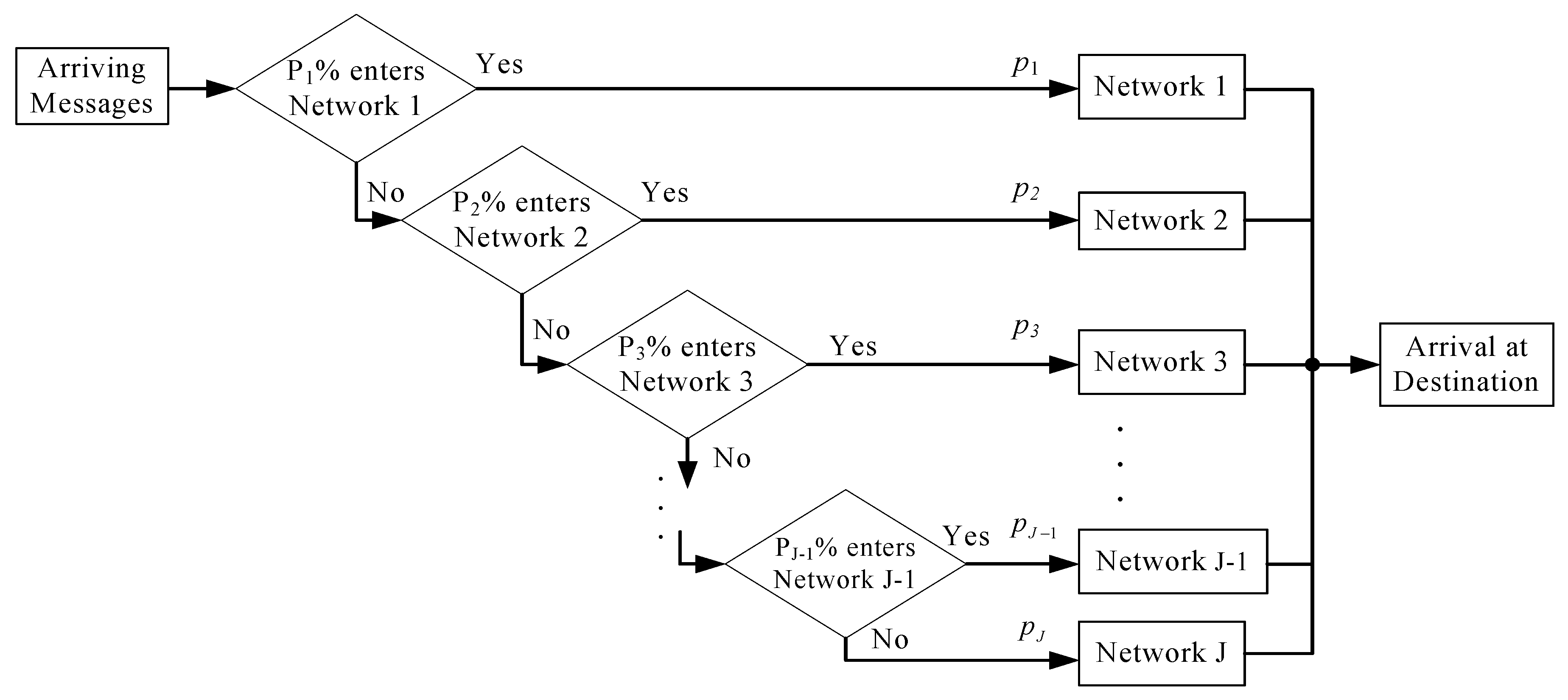
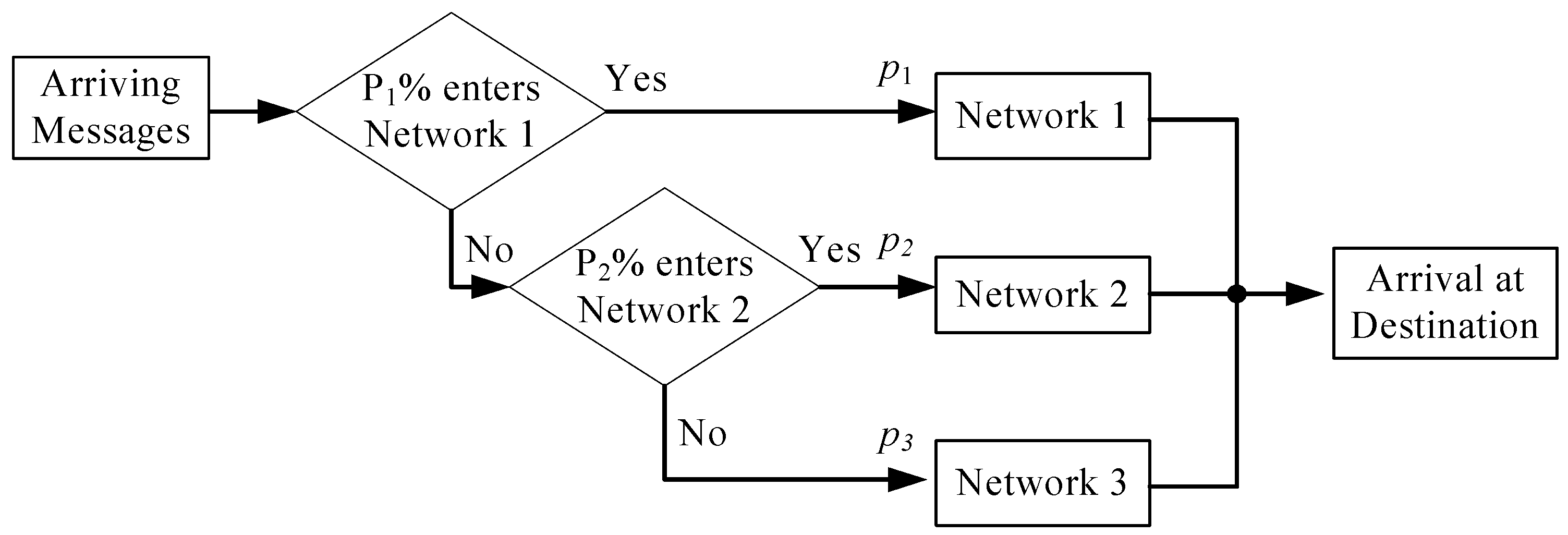
Subsequently, the OALO method is employed to minimize the operating cost of routing percentages in a communication system. The goal of queuing design optimization in a communication system is to look for the optimal routing percentages such that the expected total cost is minimal. The queuing design optimization in a communication system can be formulated as a CESOP. There are two contributions of this paper. The first one is to propose an OALO algorithm for CESOP to find a quasi-optimal design in an acceptable time. The second one is to apply the OALO algorithm to the queuing design optimization in a communication system.

The paper is organized as follows. Section 2 states the OALO algorithm to find a quasi-optimal design of CESOP. Section 3 formulates the queuing design optimization in a communication system as a CESOP. Then, the OALO is applied to resolve this CESOP. Section 4 discusses the experimental results, comparison and relevant analysis. Section 5 draws the conclusion and provides an outline on future works.

2. Integration of Ordinal Optimization with Ant Lion Optimizer

2.1. Computationally Expensive Simulation Optimization Problems

A typical CESOP can be formally stated as follows [1].

$${\underset{}{\min }}_{}f(x)=\mathrm{E}\left[G\left(r(t;x,\epsilon )\right)\right]$$

(1)

$$V\le x\le U$$

(2)

where $x={[x_1,\dots ,x_m]}^T$ denotes a m-dimensional system parameters, $f(x)$ is the objective function, $G\left(r(t;x,\epsilon )\right)$ is the performance of a simulation model, $r(t;x,\epsilon )$ denotes the trajectory of system when the simulation evolves over time, G is a function of $r(t;x,\epsilon )$ which states the performance metric of system, $\epsilon$ denotes all the randomness when it evolves during a specified sample trajectory, $V={[V_1,\dots ,V_m]}^T$ represents the lower bound, and $U={[U_1,\dots ,U_m]}^T$ denotes the upper bound. Generally, multiple replications are performed to obtain the objective value of $f(x)$. However, it is impossible to carry out a very long simulation run. A standard approach is using the sample mean to approximate the objective function, which is formally stated as follows.

$$\overline{f}(x)=\frac{1}{L}{\displaystyle \sum _{\ell =1}^L{G}_{\ell }\left(r(t;x,\epsilon )\right)}$$

(3)

where $L$ is the number of replications, and $G_{\ell }\left(r(t;x,\epsilon )\right)$ represents the objective value of the $\ell$th replication. The sample mean $\overline{f}(x)$ approximates to $f(x)$, and $\overline{f}(x)$ reaches a better result of $f(x)$ when the value of $L$ is increased. There is a major issue when the simulation problem is stochastic. Ignoring the noise in the outcomes may not only lead to an imprecise estimation, but also to potential errors in identifying the optimal solutions among those sampled. Thus, we define the precise estimation of Equation (3) when $L=L_a$, where $L_a$ denotes a sufficiently large of $L$. In addition, we define ${\overline{f}}_a(x)$ as the sample mean for a given $x$ obtained by precise estimation.

The benefit of the OO theory is the ability to separate the good designs from bad designs even with a rough model [24]. Namely, the order of performance is relatively immune to large approximation errors. Thus, an approximation model can be treated as a rough model to evaluate a design quickly. Then, an efficient optimization technique assisted by this approximation model is utilized to find N exceptional designs from solution space within an accepted computation time. The approximation model is based on the MARS [28], and the optimization technique is the RALO.

2.2. Multivariate Adaptive Regression Splines

There have been many uses of approximation models in various applications, such as the radial basis function (RBF) [30], support vector regression (SVR) [31], kriging [32], artificial neural network (ANN) [33], and multivariate adaptive regression splines (MARS) [28,29]. Among them, MARS approximates the relationship between outputs and inputs as well as interprets the relationship between the various parameters. MARS has been applied to many real-world problems, such as function approximation, curve fitting, time series forecasting, prediction and classification [29]. The main advantages of MARS include working well with a large amounts of predictor variables, automatically detecting interactions between variables, and robust to outliers. Thus, an approximation model based on the MARS is utilized to evaluate the fitness in this work.

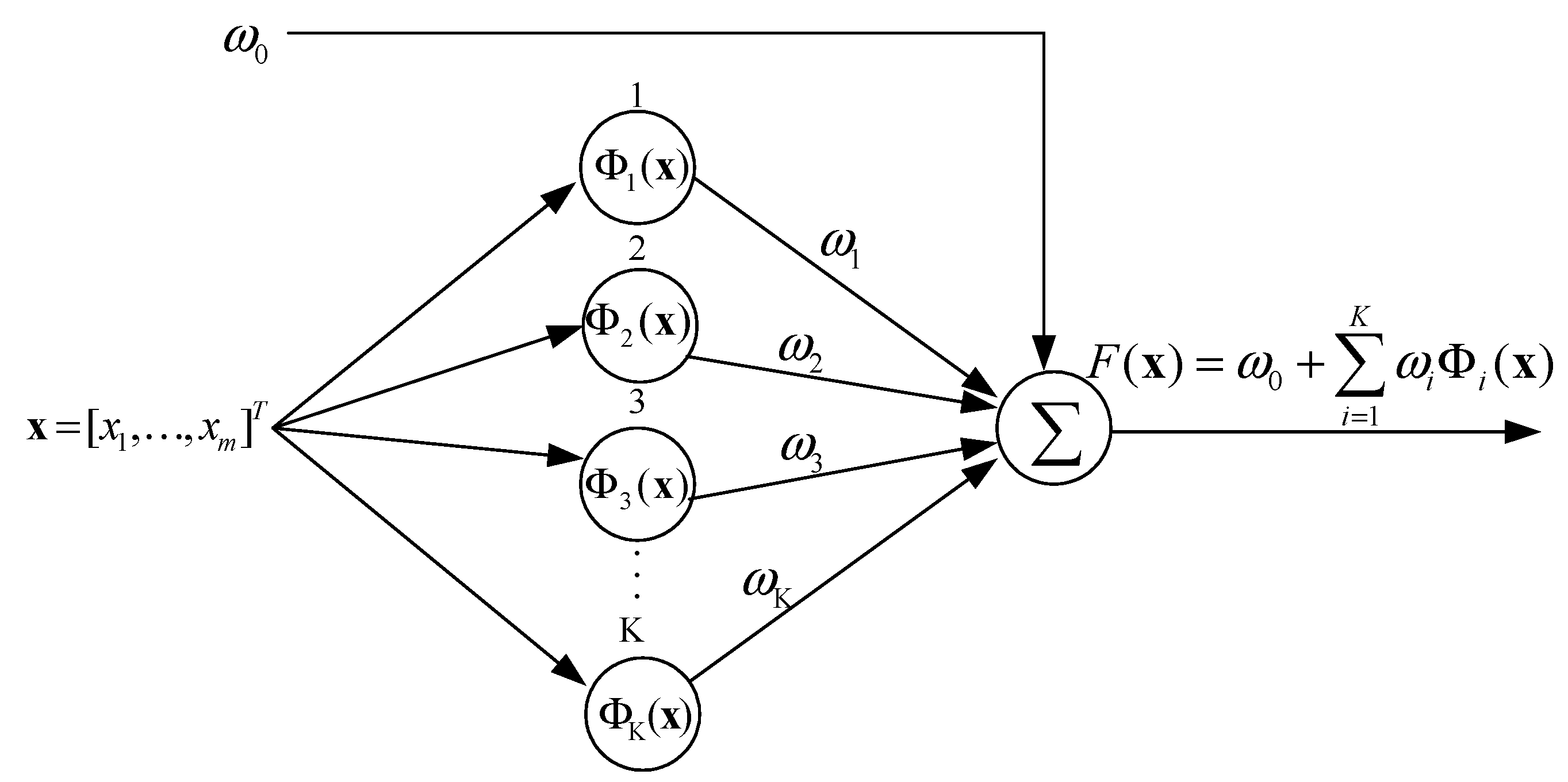
The MARS creates flexible nonlinear regression models by using separate regression slopes in distinct intervals of the independent variables. The end points of the intervals for each variable and the used variables are obtained by a very intensive searching process. The framework of MARS is demonstrated in Figure 1. The typical model of MARS is formulated as follows.

$$F(x)={\omega }_0+{\displaystyle \sum _{i=1}^{\mathrm{K}}{\omega }_i\times {\mathsf{\Phi }}_i}(x)$$

(4)

where $x$ represents an input variable, ${\omega }_0$ is an intercept coefficient, ${\omega }_i$ denotes the weight of basis functions, K indicates the amount of knots, and ${\mathsf{\Phi }}_i(\cdot )$ denotes the basis functions.

The training data patterns are ($x_i,f_a(x_i)$), where $x_i$ and $f_a(x_i)$ denote a design and their objective value obtained by precise estimation, respectively. The purpose of MARS is to make the target output $F(x)$ closer to the actual output $f_a(x)$. The optimal MARS approximation model can be obtained by two-stage process: a forward stepwise selection and a backward prune. In the selection process, MARS selects basis functions which are added to the approximation model using a fast search scheme and builds a likely large model which is overfitting the training data. The selection process terminates when the model exceeds the maximum number of basis functions. In the prune process, the overfitting model is pruned for decreasing the complexity while maintaining the overall performance in order to fit to the training data. In this process, the basis functions without appreciably increasing the residual sum of squares are deleted from the overfitting model.

MARS is trained off-line, which can be further simplified to reduce significantly the computing time for on-line. After training the MARS, the target output $F(x)$ can be calculated using simple arithmetic operations for any $x$.

2.3. Reformed Ant Lion Optimization

With the aid of the MARS approximation model, existing search approaches can be adopted to determine $N$ exceptional designs from the solution space. ALO is a biologically approach inspired by the hunting behavior of antlions and ants getting trapped in the trap set by the antlion [7]. The ALO has a high exploration capability with the help of random walk and roulette wheel to build traps. The time-varying boundary shrinking mechanism and elitism are used to increase exploitation efficiency of the ALO. There are many advantages of ALO, such as avoidance of local optima, ease of implementation, reduced need for parameter adjustment, and high precision. ALO has been successfully employed to solve the multi-robot path planning problem with obstacles [34], prediction of soil shear strength [35], and structural damage assessment [36]. Heidari et al. presented a comprehensive literature review on well-established researches of ALO from 2015 to 2018 [37]. The comparative results revealed the dominance of ALO over other SI approaches including artificial bee colony (ABC), firefly algorithm (FA), ant colony optimization (ACO), cuckoo search (CS), bat algorithm (BA), and biogeography-based optimization (BBO). With the help of random walks and roulette wheel for building traps, ALO has a high exploration capability. The shrinking of trap boundaries and elitism provide the ALO with a high exploitation efficiency. These merits make ALO to avoid immature convergence shortcomings. Accordingly, it is particularly well suited to meet the requirements in global exploration.

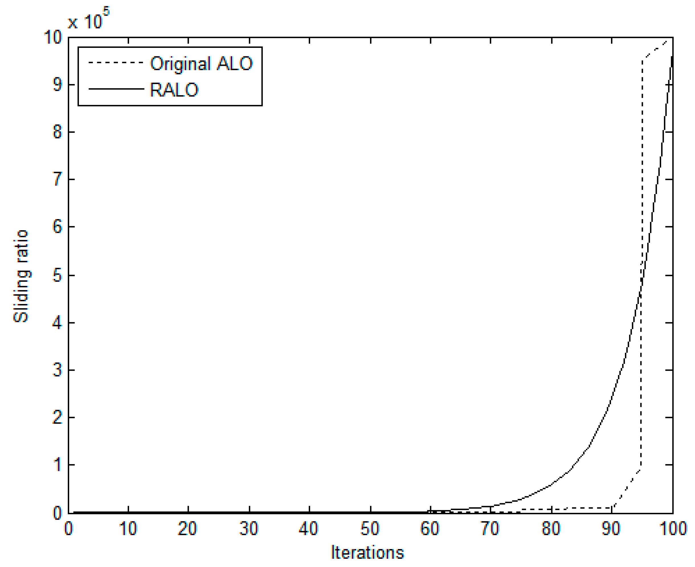
However, there are some issues of the original ALO, such as the local optima stagnation and occurrence of premature convergence for some problems. Therefore, the RALO is designed to enhance the convergent speed of the original ALO. The RALO has two self-adaptive control parameters, which are sliding factor and composition factor. The sliding factor determines the ants which are shifted toward the antlion using a given rate of slippage. The RALO uses a small value of sliding factor to increase diversification. When the sliding factor is small, the RALO intends to perform the global search. On the contrary, the RALO uses a large value of sliding factor to improve intensification. As the sliding factor is increased, the RALO intends to carry out the local search around the local optimum. The composition factor determines the degree of the elite antlion which affects the movements of all ants. The balance between exploitation and exploration of the RALO is mainly controlled by the composition factor. Large value of composition factor generates new positions of ants far from the elite antlion which will result in high exploration ability. Therefore, a large value of composition factor intends to perform exploration, while a small value leads to perform exploitation.

There are six steps of hunting prey in ALO: (i) using roulette wheel to construct antlion’s traps, (ii) random walk of ants, (iii) enter the ants to traps, (iv) adaptive shrinking boundaries of antlion’s trap, (v) catching ants and re-building traps, and (vi) performing elitism. The notations shown below are used in RALO. $\mathsf{\Psi }$ indicates the amount of ants and antlions, $k_{\max }$ is the maximum number of iterations. The position of the ith ant at iteration k is denoted by $a_i^k=[a_{i,1}^k,\dots ,a_{i,m}^k]$. The position of the ith antlion at iteration k is denoted by $x_i^k=[x_{i,1}^k,\dots ,x_{i,m}^k]$. The position of the elite antlion is denoted by $x^{*}=[x_1^{*},\dots ,x_m^{*}]$. $w^k$ is a sliding factor at iteration k, $w^k\in [w_{\min },w_{\max }]$, where $w_{\min }$ and $w_{\max }$ indicate the minimum and maximum value, respectively. ${\alpha }^k$ is a composition factor at iteration k, ${\alpha }^k\in [{\alpha }_{\min },{\alpha }_{\max }]$, where ${\alpha }_{\min }$ and ${\alpha }_{\max }$ represent the minimum and maximum value, respectively. The pseudo-code of RALO is represented in Algorithm 1.

Algorithm 1: Pseudo-code of the R ALO algorithm.

Input: Amount of ants and antlions, range of two control parameters and maximum number of iterations ($k_{\max }$).

Output: The best antlion.

Initialize the positions of all ants $a_i^0$ and antlions $x_i^0$ inside V and U bounds.

Evaluate the fitness of all antlions by MARS.

Determine the elite antlion $x^{*}$.

while $k\le k_{\max }$ do

for an ant $a_i^k$ do

Choose an antlion $x_i^k$ using the roulette wheel.

Random walk of $a_i^k$ nearby antlion $x_i^k$ to generate $R_S^{k+1}$

Random walk of $a_i^k$ nearby elite antlion $x^{*}$ to generate $R_E^{k+1}$

Update the minimum and maximum of each design variable.

Update the position of $a_i^{k+1}$ based on $R_S^{k+1}$ and $R_E^{k+1}$

End for

Evaluate the fitness of all ants and antlions by MARS.

Replace an antlion with it corresponding ant.

Update sliding factor and composition factor.

Update the elite antlion.

End while

The steps involved in the RALO Algorithm 2 are briefly explained below.

Algorithm 2: The RALO

Step  1: Configuring basic parameters (a) Setting the values of $\mathsf{\Psi }$, $w_{\min }$,$w_{\max }$, ${\alpha }_{\min }$, ${\alpha }_{\max }$ and $k_{\max }$. (b) Set $u_j^0=U_j$, $v_j^0=V_j$, $j=1,\dots ,m$. Let $k=0$, where $k$ indicates the iteration index. Step  2: Initializing a population (a) A population containing Ψ ants and Ψ antlions are generated. $$a_{i,j}^0=V_j+\lfloor rand[0,1]\times (U_j-V_j)\rfloor , i=1,\dots ,\mathsf{\Psi }, j=1,\dots ,m$$ (5) $$x_{i,j}^0=V_j+\lfloor rand[0,1]\times (U_j-V_j)\rfloor , i=1,\dots ,\mathsf{\Psi }, j=1,\dots ,m$$ (6) where $rand[0,1]$ indicates a random number in range from 0 to 1, and Vj and Uj express the lower and upper bound, respectively. (b) Calculate the fitness $F(x_i^0)$ of antlion assisted by MARS, $i=1,\dots ,\mathsf{\Psi }$. Step  3: Ranking Rank the Ψ antlions based on the fitness from the smallest to the largest, and determine the elite antlion $x^{*}=[x_1^{*},\dots ,x_m^{*}]$. Step  4: Random walk of ants Generate new position of each ant. $$a_{i,j}^{k+1}=\frac{\left(a_{i,j}^k-\min {\mathrm{R}}_{i,j}\right)\times (u_j^k-v_j^k)}{\max {\mathrm{R}}_{i,j}-\min {\mathrm{R}}_{i,j}}+v_j^k, i=1,\dots ,\mathsf{\Psi }, j=1,\dots ,m$$ (7) where ${\mathrm{R}}_{i,j}=[0,cusum(binrn{d}^1),\dots ,cusum(binrn{d}^k),\dots ,cusum(binrn{d}^{k_{\max }})]$, cusum refers to the cumulative sum, $binrn{d}^k$ denotes the random number at iteration k, either 1 or −1, $\max {\mathrm{R}}_{i,j}$ and $\min {\mathrm{R}}_{i,j}$ denote the minimum and maximum random walk of the j-th variable for the i-th ant, respectively, $u_j^k$ and $v_j^k$ express the minimum and maximum of the j-th variable at iteration k. Step  5: Slide ants in a trap (a) Update the minimum and maximum of the j-th variable. $$v_j^{k+1}=\{\begin{array}{c}{x}_j^k+\frac{v_j^k}{{10}^{w^k\times (}{}^{k/k_{\max })}},rand[0,1]>0.5\\ x_j^k-\frac{v_j^k}{{10}^{w^k\times (}{}^{k/k_{\max })}},rand[0,1]\le 0.5\end{array}, j=1,\dots ,m$$ (8) $$u_j^{k+1}=\{\begin{array}{c}{x}_j^k+\frac{u_j^k}{{10}^{w^k\times (}{}^{k/k_{\max })}},rand[0,1]>0.5\\ x_j^k-\frac{u_j^k}{{10}^{w^k\times (}{}^{k/k_{\max })}},rand[0,1]\le 0.5\end{array}, j=1,\dots ,m$$ (9) where $w^k$ denotes the sliding factor at iteration k, $u_j^k$ and $v_j^k$ express the minimum and maximum of the j-th variable at iteration k, $x_j^k$ is the j-th antlion position at iteration k, which can be either antlion $x{s}_j^k$ selected by the roulette wheel or the elite antlion $x_j^{*}$ determined by the following equation. $$x_j^k=\{\begin{array}{c}x{s}_j^k,rand[0,1]>0.5\\ x_j^{*},rand[0,1]\le 0.5\end{array}, j=1,\dots ,m$$ (10) (b) Update positions of all ants. $$a_i^{k+1}={\alpha }^k\times R_S^{k+1}+(1-{\alpha }^k)\times R_E^{k+1}, i=1,\dots ,\mathsf{\Psi }$$ (11) where αk denotes the composition factor at iteration k, $R_S^{k+1}$ denotes the random walk around an antlion which is selected by the roulette wheel at iteration k + 1, $R_E^{k+1}$ denotes the random walk around the elite antlion at iteration k + 1. Step  6: Calculate the fitness Calculate the fitness $F(a_i^{k+1})$ of ant $a_i^{k+1}$ and the fitness $F(x_i^{k+1})$ of antlion $x_i^{k+1}$ assisted by MARS, $i=1,\dots ,\mathsf{\Psi }$. Step  7: Replace an antlion with it corresponding ant Apply the greedy selection between $a_i^{k+1}$ and $x_i^{k+1}$. If $F(a_i^{k+1})<F(x_i^{k+1})$, then set $x_i^{k+1}=a_i^{k+1}$, $i=1,\dots ,\mathsf{\Psi }$. Step  8: Update sliding factor and composition factor. $$w^{k+1}=w_{\min }+(w_{\max }-w_{\min })\times \left(1-\exp \left(-\frac{w_{\max }}{w_{\min }}\times \frac{k+1}{k_{\max }}\right)\right)$$ (12) $${\alpha }^{k+1}={\alpha }_{\min }+\left({\alpha }_{\max }-{\alpha }_{\min }\right)\times \exp \left(\ln {\left(\frac{{\alpha }_{\min }}{{\alpha }_{\max }}\right)}^2\times \frac{k+1}{k_{\max }}\right)$$ (13) Step  9: Elitism Apply the greedy selection between $x_i^{k+1}$ and $x^{*}$. If $F(x_i^{k+1})<F(x^{*})$, then set $x^{*}=x_i^{k+1}$, $i=1,\dots ,\mathsf{\Psi }$. Step  10: Stop criteria If $k\ge k_{\max }$, then stop; else, let $k=k+1$ and return to Step 4.

The RALO terminates when it reaches a specified maximum number of iterations $k_{\max }$. When the RALO has stopped, the final $\mathsf{\Psi }$ antlions are ranked according to the fitness. Then, the former $N$ antlions are selected as the exceptional designs.

2.4. Ranking and Selection

We continue to determine the quasi-optimal design from the $N$ exceptional designs using the R&S procedure. The main idea of the R&S procedure is spending more computing efforts on few critical designs and less on most non-critical designs. The proposed R&S procedure composes of multiple stages, which select and allocate the most computational budget to critical designs that has a high probability to be the quasi-optimal design. The number of critical designs in each stage is decreased gradually. Remaining designs are continuing to perform simulation and some of them are eliminated in each stage, and the best one obtained in the last stage is the quasi-optimal design. The computational complexity can be gradually reduced, because the number of the critical designs had been greatly decreased when the evaluations are more refined.

The more refined evaluations used in those stages are simulation with various numbers of replications ranging from tiny to large. First, we choose an initial amount of replications as $L_0$. The amount of replications and the amount of critical designs in the $i$th stage are denoted as $L_i$ and $N_i$, respectively. We set $L_i=e{L}_{i-1}$ (or $L_i=e^i{L}_0$) for $i=1,2,\dots$., and $N_i=N_{i-1}/e$ (or $N_i=N_1/e^{i-1}$) for $i=2,3,\dots$, where $N_1=N$. The Monte Carlo simulation with exponential rate provides a substantial computational speed-up without noticeable overshoot of the Probability of Correct Selection (PCS). The value of the $N_i$ is rounded to the nearest integer. The number of stages, denoted as $n_s$, is obtained by

$$n_s=\arg \{\underset{n_s}{\min }(L_0\times e^{n_s-1}\le L_a<L_0\times e^{n_s}{,}_{}1\le N/e^{n_s-1}<N_{\min })\}$$

(14)

where $L_a$ denotes the amount of replications in precise estimation, and $N_{\min }$ denotes the specified minimum size of selected subset. Equation (14) determines $n_s$ by satisfying at least one of the following two conditions: (i) the value of $L_{n_s}$ in the last stage exceeds the value of precise estimation, i.e., $L_{n_s}$ > $L_a$, and (ii) the size of selected subset in the last stage is smaller than the specified minimum size, i.e., $N_{n_s}<N_{\min }$. When the value of $n_s$ is obtained, a simulation with $L_i=e^i\times L_0$ replications is adopted to calculate $\overline{f}(x)$ in the $i$-th stage. Next, these $N/e^{i-1}$ critical designs are ranked based on the value of $\overline{f}(x)$ and the former $N/e^i$ critical designs are selected into the selected subset for the ($i+1$)-th stage. A simulation with $L_a$ replications is adopted to calculate ${\overline{f}}_a(x)$ of all $N_{n_s}$ critical designs in the last stage. The critical design with the smallest ${\overline{f}}_a(x)$ in the last stage is the quasi-optimal design.

2.5. The OALO Algorithm

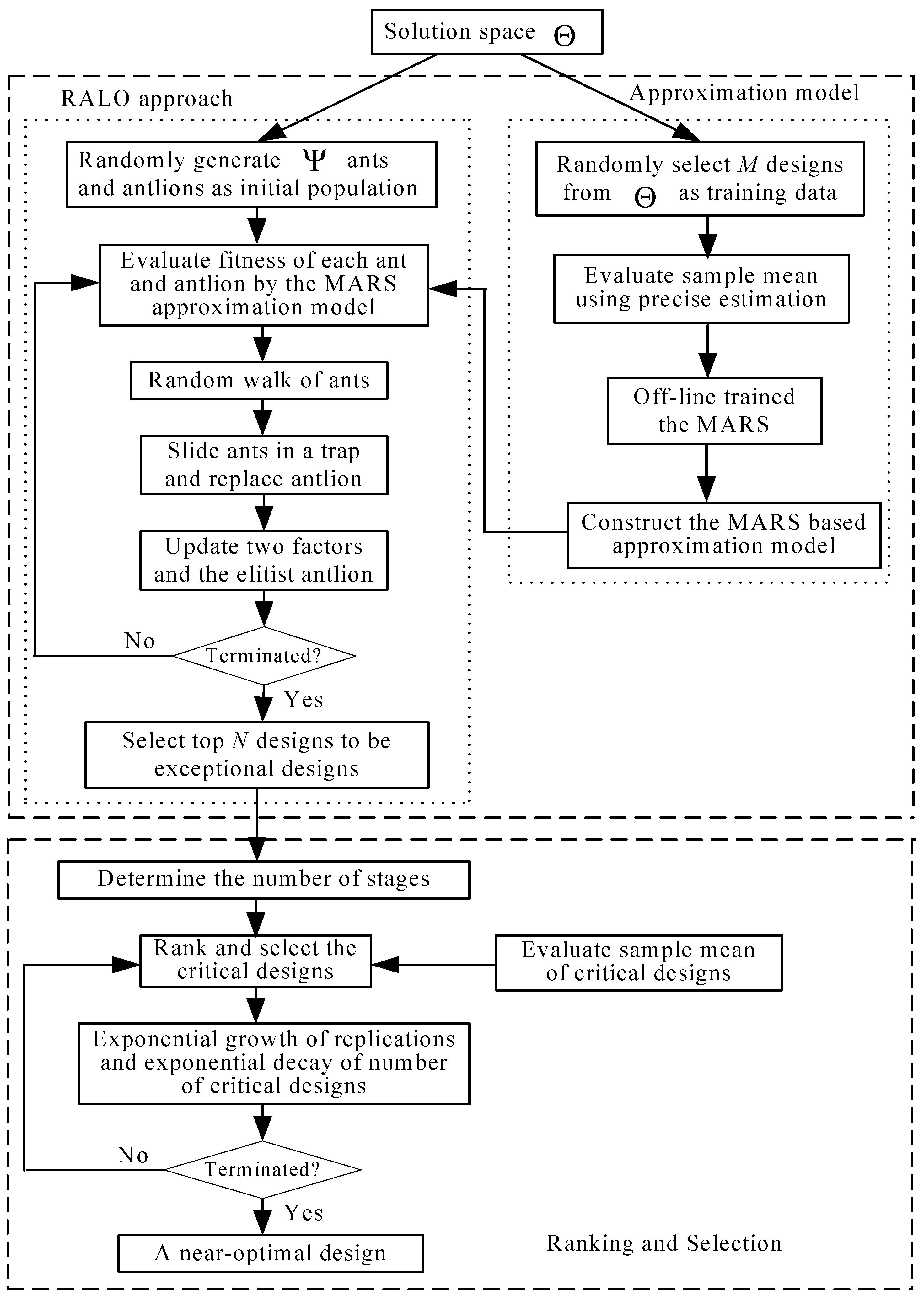
The OALO algorithm can be expressed by the flow diagram as shown in Figure 2. Described below are the step-wise procedures of the OALO Algorithm 3.

Algorithm 3: The OALO.

Step  0: Set the values of $M,\mathsf{\Psi },w_{\min },w_{\max }, {\alpha }_{\min }, {\alpha }_{\max }, k_{\max }, N, L_0, L_a \mathrm{and} N_{\min }$ Step  1: Randomly choose M x’s from solution space and calculate $f_a(x)$, then train the MARS off-line using these M designs. Step  2: Randomly yield Ψ ants a’s and antlions x’s as the initial population and adopt Algorithm 2. After Algorithm 2 terminates, rank all the final Ψ x’s based on their approximate fitness from the lowest to the highest and choose the prior N x’s to be the N exceptional designs. Step  3. Decide the number of stages, $n_s$, of the R&S procedure. Step  4. For i = 1 to $n_s-1$, perform the simulation with replications $L_i=e^i{L}_0$ to estimate $\overline{f}(x)$ of the $N_i=N/e^{i-1}$ designs in the i-th stage. Rank these $N/e^{i-1}$ designs based on their $\overline{f}(x)$ and select the former $N/e^i$ designs as the critical designs for the (i + 1)-th stage. Step  5. Perform the simulation with replications $L_a$ to calculate ${\overline{f}}_a(x)$ of the $N/e^{n_s-1}$ designs. The design with the smallest ${\overline{f}}_a(x)$ is the quasi-optimal design.

3. Optimization of a Communication System

3.1. Problem Statement

Queueing designs play an important role in managing communication system between different components of a large-scale distributed system [38]. The optimal routing optimization in design of queueing networks is a challenging problem that arises in many real-life situations. Such questions are arising in management of computer systems and data networks. In the last few decades, there has been an upsurge of interest in the system modeling methods, such as discrete-event simulation and queueing theory. In general, the discrete-event simulation can enable the modeling of system operation control [39]. Unlike discrete-event simulation, queueing theory requires very little data and obtains the relatively simple formula to predict various performance measures. In designing queueing systems, it is important to have a good balance between service to messages and economic considerations. Queues happen when there are limited resources for providing a service. In essence, all queuing systems are broken down into the entities queuing for an activity, e.g., dispensing and counseling. The goal of queuing design optimization in a communication system is to look for the optimal routing percentages for minimizing the expected total cost.

Consider a queueing network design situation consisting of a communication system, one should determine the routing percentages to route randomly arriving messages to a particular destination [40]. There are n arrived random messages that need to go to a particular destination and there are J networks available to process these messages. Figure 3 shows an example of queueing network design with J networks. The per message processing cost is $c_1,c_2,\dots ,c_{\mathrm{J}}$ depending on which network the message is routed through. It also takes time for a message to go through a network. This transit time is denoted by $t_j$ for each network j, where $t_j$ follows a triangular distribution with a mean $u_j$, lower limit $u_j-0.5$ and upper limit $u_j+0.5$. There is a cost for the length of time a message spends in a network measured by K per unit time. The decision variables are the routing percentages ${\mathrm{P}}_1,{\mathrm{P}}_2,\dots ,{\mathrm{P}}_{\mathrm{J}-1}$ $\in$ [0, 100] which are the probabilities that a message will go through a particular network. When a message is in front of network j, there is a ${\mathrm{P}}_j$% chance that it will be processed by network j. If the message is not processed by that network, then it will go to network j + 1, and will be processed with probability ${\mathrm{P}}_{j+1}$%, and so on. All messages arrive at network 1 with an exponentially distributed interarrival time with a mean of 1/λ time unit. The average transit time on the network j is $\mathrm{E}[t_j]$ in steady state. The goal is to minimize the expected total cost, which is the sum of processing cost and average transit cost.

3.2. Mathematical Formulation

The optimization of queueing network design can be formulated as a CESOP.

$${\underset{x\in \mathsf{\Theta }}{\min }}_{}f(x)={\displaystyle \sum _{j=1}^{\mathrm{J}}n\times p_j\times (c_j+\mathrm{K}\times \mathrm{E}[t_j])}$$

(15)

Subject to

$$p_1={\mathrm{P}}_1/100$$

(16)

$$p_j=\left({\mathrm{P}}_j/100\right)\times \left(1-p_{j-1}\right), j=2,\dots ,\mathrm{J}-1$$

(17)

$$p_N=1-{\displaystyle \sum _{j=1}^{J-1}{p}_j}$$

(18)

where $x={[P_1,\dots ,P_{\mathrm{J}-1}]}^T$ denotes a J−1 dimensional design vector, $f(x)$ is the expected total cost, $P_j\in [0,100]$ denotes the routing percentage, $\mathsf{\Theta }={[0,100]}^{\mathrm{J}-1}$ denotes the feasible region, n is the number of messages, $c_j$ denotes per message processing cost of network j, K denotes transit cost, and $\mathrm{E}[t_j]$ denotes the average transit time on the network j in steady state.

The goal of the CESOP is to find the optimal routing percentages, $x^{\ast }$, such that the expected total cost is minimum. Generally, multiple simulation replications are performed to obtain the objective value. Thus, the sample mean is utilized to approximate the objective value.

$$\overline{f}(x)=\frac{1}{L}{\displaystyle \sum _{\ell =1}^L{f}_{\ell }(x)}$$

(19)

$$f_{\ell }(x)={\displaystyle \sum _{j=1}^{\mathrm{J}}n\times p_i\times (c_i+K\times t_j^{\ell })}$$

(20)

where $L$ denotes the amount of replications, $f_{\ell }(x)$ represents the objective value of the $\ell$th replication, and $t_j^{\ell }$ denotes the transit time on the network j of the $\ell$th replication. For simplicity, we let ${\overline{f}}_a(x)$ indicate the sample mean for a given $x$ using precise estimation.

Figure 4 shows the relationship between inputs and output in queueing network design, where $x$ expresses the design vector, $\lambda$ denotes the arrival rate of messages, $L$ indicates the number of replications, and $\overline{f}(x)$ is the sample mean.

3.3. Apply the OALO Algorithm

3.3.1. Establish the Approximation Model

Various basis functions in different intervals of the input variables space are used to build the MARS approximation model. The output of MARS $F(x)$ is predicted by a linear function, which is composed of an intercept constant and weighted basis functions. To obtain the optimal MARS approximation model, we need to determine the intercept constant and expansion coefficients of basis functions. There are four steps to establish the MARS approximation model for roughly estimating a design vector. (i) Randomly select $M$ $x$’s from solution space and calculate ${\overline{f}}_a(x)$ by precise estimation. (ii) Express the $M$ design vectors and the corresponding sample means as $x^{(i)}$ and ${\overline{f}}_a(x^{(i)})$, respectively. (iii) The optimal MARS approximation model is constructed using a two-stage process. (iv) The ordinary least squares method is utilized to calculate the coefficient of each term.

The following hinge function is adopted as the basis function in the MARS approximation model.

$${\mathrm{B}}_m(x)={{\displaystyle {\displaystyle \prod _{k=1}^{K_m}\left[s_{k,m}\times \left(x_{v(k,m)}-l_{k,m}\right)\right]}}}_{+}$$

(21)

where $k_m$ denotes the amount of splits corresponding to the mth basis function, $s_{k,m}=\pm 1$, $v(k,m)$ is the v-th variable, $1\le v\le n$, n indicates the dimension of $x$, $x_{v(k,m)}$ is the variable split, and $l_{k,m}$ denotes a knot. The ‘+’ subscript indicates that a truncated function is used in the associated bracketed term.

$${\left[s_{k,m}\times \left(x_{v(k,m)}-l_{k,m}\right)\right]}_{+}^{}=\{\begin{array}{c}{s}_{k,m}\times \left(x_{v(k,m)}-l_{k,m}\right){,}_{}i{f}_{}{s}_{k,m}\times \left(x_{v(k,m)}-l_{k,m}\right)>0\\ 0{,}_{}otherwise\begin{array}{cccc}\begin{array}{cccc}\begin{array}{cc}\begin{array}{cc}& \end{array}& \end{array}& & & \end{array}& & & \end{array}\end{array}$$

(22)

MARS finds possible univariate candidate knots and across interactions among all variables. The selected input variables and knot locations are obtained using an exhaustive search algorithm. A “loss of fit” (LOF) criterion is utilized to optimize predictors, knots and interactions simultaneously. MARS chooses the LOF which most improves the approximation model at each search process.

3.3.2. Apply the RALO

With the assistance of MARS approximation model, $N$ exceptional designs can be quickly chosen from solution space using the RALO. At first, $\mathsf{\Psi }$ ants and antlions are arbitrarily created as the initial population. Since the decision variables are the routing percentages with a range of 0–100%, the positions of ants and antlions in initial population are randomly generated by $U[0,100]$, where $U[0,100]$ is a uniformly distributed random variable that ranges between 0 and 100. The fitness of each ant and antlion is obtained by the MARS approximation model. After the RALO executed $k_{\max }$ iterations, the final $\mathsf{\Psi }$ antlions are sorted based on their fitness. When a real value of the optimal design variable is obtained, we can round this real value to the nearest integer using the rounding function $z_{j,k}^i=\lfloor x_{j,k}^i\rfloor$, where $x_{j,k}^i\in \Re$ and $z_{j,k}^i\in Z$. Finally, we choose the former $N$ antlions to construct the candidate subset. The value of N may not be large to save computational effort; however, some critical designs may be lost when the value of N is small.

3.3.3. Obtain the Quasi-Optimal Design

Finally, the R&S technique is utilized to find a quasi-optimal design from the $N$ exceptional designs. First, we define the values of $L_0$, $L_a$, $N_{\min }$ and calculate the value of $n_s$ by Equation (14). For $i=1$ to $n_s-1$, a stochastic simulation with $L_i=e^i\times L_0$ replications is performed to compute $\overline{f}(x)$ of the $N_i=N/e^{i-1}$ critical designs. Then, we rank these $N/e^{i-1}$ critical designs based on their $\overline{f}(x)$ and select the former $N/e^i$ critical designs as the selected subset for the ($i+1$)-th stage. Finally, a stochastic simulation with $L_a$ replications is performed to calculate ${\overline{f}}_a(x)$ of all $N/e^{n_s-1}$ critical designs in the last stage. The critical design with the smallest ${\overline{f}}_a(x)$ is the quasi-optimal design.

4. Experimental Results

4.1. Test Examples and Simulation Results

Two problems presented in [41] are utilized to test the performance of the OALO algorithm. The first problem is a small example with 3 networks as shown in Figure 5. The number of messages is n = 1000. The cost per unit time in system is K = $0.005. The processing costs per service are $0.03 for network 1, $0.01 for network 2 and $0.005 for network 3. The message interarrival times have an exponential distribution with mean $1/\lambda$ = 1 time unit. The means of transit time are ${\mu }_j$ = 1, 2, and 3 for networks 1, 2, and 3, respectively. The second problem is a large example with 10 networks. The number of messages is n = 1000. The cost per unit time in system is K = $0.005. The processing cost per service for network j is $c_j=1/j,j=1,\dots ,10$. The interarrival rate of messages is $\lambda$ = 1. The mean of transit time through network j is ${\mu }_j=j,j=1,\dots ,10$.

In small example, the MARS was trained by randomly sampling M = 384 designs. The amount M = 384 was produced using the sample size formula for a 95% confidence level and a 5% confidence interval [42]. The number of sampling designs depends on the parameters and complexity of the trained MARS model. For MARS, the performance is expected to reach a maximum threshold no matter how much more data is included in the training. In other words, there is a point where more data may not improve the model. Accordingly, the additional samples become redundant when the value is larger than 384. The objective value of each design was estimated using precise estimation.

Due to the random nature of stochastic simulation process, 30 trials (complete repetitions of the entire experiment) were carried out to check the consistency. After running multiple experimental trials with different settings, the parameter settings in RALO for small example were ${\alpha }_{\max }=0.8$, ${\alpha }_{\min }=0.2$, $w_{\max }=6$ $w_{\min }=1.5$, $\mathsf{\Psi }=20$ and $k_{\max }=100$. There is no existing systematic way to determine the preferable ranges of the two control parameters, $[{\alpha }_{\min },{\alpha }_{\max }]$, $[w_{\min },w_{\max }]$ and the value of $N$. Although a proper parameter setting can obtain a good performance, however such setting is problem dependent. Thus, the preferable ranges of $[{\alpha }_{\min },{\alpha }_{\max }]$, $[w_{\min },w_{\max }]$ and the value of $N$ were determined using a series of hand-tuning experiments after analyzing the influence on solution accuracy and convergence rate.

The values of α and w were dynamically adjusted to strengthen exploration in early iterations and exploitation in later iterations. Figure 6 displays the variations of α and w over iterations. The function of α is an exponentially decreasing function. A large value of α tends to favor and promote exploration at the beginning, however, a small value of α increases the local search tendency which leads to fast convergence speed. The function of w is an exponentially increasing function. A small value of w achieves diversity more efficiently or effectively. When the optimization processes proceed, the value of w is exponentially increased to gradually improve local exploitation. Figure 7 presents the sliding ratio between original ALO and RALO. The value of exceptional designs was N = 10. The parameter settings in R&S for small example were $L_0$ = 50, $N_{\min }$ = 2, $L_a={10}^3$, and $n_s$ = 3.

Table 1. The quasi-optimal design $x^{*}$, cost and the CPU times of the best run in small example.

$x^{*}$	Cost	CPU Times (s)
[54, 64]T	32.59	18.52

shows the quasi-optimal design $x^{*}$, cost and the central processing unit (CPU) times of the best run among the 30 trials in small example.

In large example, the MARS was trained by randomly sampling M = 9604 designs. The amount M = 9604 was produced using the sample size formula for a 95% confidence level and a 1% confidence interval. The sample mean of each design was estimated using precise estimation. After running multiple experimental trials with different settings, the parameter settings in RALO for large example were ${\alpha }_{\max }=0.9$, ${\alpha }_{\min }=0.1$, $w_{\max }=6$ $w_{\min }=1$, $\mathsf{\Psi }=200$ and $k_{\max }=1000$. The value of exceptional designs was N = 100. The parameter settings in R&S for large example were $L_0$ = 10, $N_{\min }$ = 2, $L_a={10}^3$, and $n_s$ = 5.

Table 2. Number of critical designs and replications in each stage.

Stage i	1	2	3	4	5
$N_i$	100	37	14	5	2
$L_i$	27	74	201	546	1000

demonstrates the amount of critical designs and replications in each stage. Since the parameter settings in R&S are irrelevant to the random nature of stochastic simulation process, the values listed in Table 2 are applied to the 30 trials.

Table 3. The quasi-optimal design $x^{*}$, cost and the consumed CPU time of the best run in large example.

$x^{*}$	Cost	CPU Times (s)
[2, 2, 2, 16, 26, 16, 19, 17, 10]T	270.75	98.27

shows the quasi-optimal design $x^{*}$, cost and the CPU times of the best run among the 30 trials in large example. Since the MARS is trained off-line, its training time is not included in the CPU time consumed by the OALO in Table 1 and Table 3. The CPU time contains the computing effort consumed by the RALO and R&S procedure. The CPU time was less than 100 s for all trials which were fast enough to meet the specification for real time applications. The stochastic simulation process can be used in optimal queuing design of a communication system with any distribution of arrival rates, even for high-dimension problems.

Based the large deviation theory, the OALO can achieve an exponential convergence rate in stochastic simulation models. Detail convergence analysis can refer to Chap 2.4 in [24] for detailed proof. The proposed OALO method can be applied to more complex simulation-based optimization problems, such as optimal reinsurance-investment problems, multiskill call center with preference lists, flow lines with multiple-products, and portfolio optimization problems with real-world constraints. The benefit of the OALO method is to reduce the required simulation time significantly by determining quasi-optimal design instead of finding the best design. Nevertheless, yielding a candidate subset of designs may not be very satisfactory in some cases. The drawback of the OALO method is that it does not provide an absolute guarantee of the global optimality.

4.2. Comparisons

To test the quality and efficiency of the OALO algorithm, three competing approaches, GA, ES and particle swarm optimization (PSO), were adopted to solve the large example. In the employed GA [43], the size of population was 200. An integer-valued solution was represented by a real-valued coding. A crossover rate of 0.9 and a mutation rate of 0.05 were employed. In the applied ES [44], the self-adaptation rate was $1/\sqrt{9}$. The size of population was 200 and the size of offspring was 400. In the applied PSO [45], the size of population was 200. Both cognitive and social factors were 2.05. The allowed maximum velocity was 0.5 and the inertia weight was 1. The precise estimation was used to calculate the sample mean of thee competing methods.

Due to the uncertainty of the large example, 30 trials were simulated. For a type of statistical analysis, the modern standard is 30 trials to give an acceptable statistical precision. Since three competing approaches should consume a long time to yield the optimum, the iterative optimization procedures were terminated when they had spent 60 min of computing time.

Table 4. Comparison of four approaches over 30 simulation trials.

Methods	ABSM †	$\frac{\mathrm{ABSM}-{\ast }^{{}^{\S }}}{*}\times 100\%$
OALO	270.75	0
GA using precise estimation	296.55	9.53%
ES using precise estimation	294.63	8.82%
PSO using precise estimation	286.16	5.69%

^†ABSM: average best-so-far sample mean; ^§ *: ABSM of OALO.

lists the average best-so-far sample means obtained using GA, ES and PSO, whose values were 9.53, 8.82, and 5.69% more than that computed using OALO, respectively. Test results reveal that the OALO algorithm can obtain the quasi-optimal designs within a reasonable time as well as outperforms three competing approaches.

Furthermore, the solution quality of the proposed OALO is of interest. To verify the global optimality, the ranks of the solutions obtained from four methods were analyzed. Since it is difficult to analyze the ranks of all solutions, a representative subset, $\mathsf{\Omega }$, is selected to accurately reflect the characteristics of the large solution space. Because the solution space is large, 16,641 samples were randomly selected from entire solution space to build the representative subset. Then, the precise estimation was employed to calculate the corresponding sample means. The size of the representative subset, $\left|\mathsf{\Omega }\right|$ = 16,641, was produced using the sample size formula for a 99% confidence level and a 1% confidence interval [42].

An analytic process concerning ranking percentage was executed to reveal the rank of a quasi-optimal solution in the representative subset. The ranking percentage of a quasi-optimal solution in $\mathsf{\Omega }$ is defined by $\frac{rk}{\left|\mathsf{\Omega }\right|}\times 100\%$, where $rk$ denotes the rank of a quasi-optimal solution.

Table 5. Statistics obtained by four methods over 30 simulation trials.

Methods	Min.	Max.	Mean	S.D.	S.E.M.	Average Ranking Percentage
OALO	270.01	271.59	270.75	0.3	0.0548	0.002%
GA using precise estimation	289.78	303.11	296.55	2.7	0.493	0.975%
ES using precise estimation	291.29	299.44	294.63	1.8	0.3286	0.637%
PSO using precise estimation	283.94	289.13	286.16	1.2	0.2191	0.592%

lists the statistics related to the average best-so-far sample means and average ranking percentages over 30 trials using four methods. The standard deviation (S.D.) and standard error of mean (S.E.M.) concerning the average best-so-far sample means obtained by OALO over 30 trials were 0.3 and 0.0548, respectively. These small values indicate that most of the sample means of the OALO are very close to the optimum over 30 trials. In other words, the OALO algorithm can usually reach near-optimum even though no guarantee of actually obtaining the global optimum.

5. Conclusions

To solve the CESOP within a reasonable time, a heuristic algorithm integrating OO with ALO was developed. The OALO algorithm comprises three parts including approximation model, global exploration and local exploitation. The MARS approximation model was used to evaluate a design quickly. The OALO algorithm adopted the RALO for global exploration with the R&S procedure for local exploitation. The OALO algorithm was applied to minimize the expected cost of optimal queuing design in a communication system, which was formulated as a CESOP. The OALO algorithm was compared with three competing methods—GA, ES and PSO, using precise estimation. The quasi-optimal design that was determined by the OALO algorithm has a high solution quality with beneficial computational efficiency. Simulation results reveal that most of the objective values for the OALO algorithm are close to the optimum over 30 trials. The OALO algorithm usually reach near-optimum even though no guarantee of actually obtaining the global optimum. Future research direction should be applying the OO theory to solve more complex stochastic simulation optimization problems, such as optimal reinsurance-investment problems and portfolio optimization problems with real-world constraints.

References

1. Li, M.; Sadoughi, M.; Hu, C.; Hu, Z.; Eshghi, A.T.; Lee, S. High-Dimensional Reliability-Based Design Optimization Involving Highly Nonlinear Constraints and Computationally Expensive Simulations. J. Mech. Des. 2019, 141, 051402. [Google Scholar] [CrossRef]
2. Jiang, P.; Cheng, J.; Zhou, Q.; Shu, L.S.; Hu, J.X. Variable-fidelity lower confidence bounding approach for engi-neering optimization problems with expensive simulations. AIAA J. 2019, 57, 5416–5430. [Google Scholar] [CrossRef]
3. Yuan, G.L.; Wei, Z.X.; Yang, Y.N. The global convergence of the Polak-Ribiere-Polyak conjugate gradient algo-rithm under inexact line search for nonconvex functions. J. Comput. Appl. Math. 2019, 362, 262–275. [Google Scholar] [CrossRef]
4. Hussain, K.; Salleh, M.N.M.; Cheng, S.; Shi, Y. On the exploration and exploitation in popular swarm-based metaheuristic algorithms. Neural Comput. Appl. 2019, 31, 7665–7683. [Google Scholar] [CrossRef]
5. Ryerkerk, M.; Averill, R.; Deb, K.; Goodman, E. A survey of evolutionary algorithms using metameric represen-tations. Genet. Program. Evolvable Mach. 2019, 20, 441–478. [Google Scholar] [CrossRef]
6. Yang, X.-S.; Deb, S.; Zhao, Y.-X.; Fong, S.; He, X. Swarm intelligence: Past, present and future. Soft Comput. 2018, 22, 5923–5933. [Google Scholar] [CrossRef] [Green Version]
7. Mirjalili, S. The Ant Lion Optimizer. Adv. Eng. Softw. 2015, 83, 80–98. [Google Scholar] [CrossRef]
8. Assiri, A.S.; Hussien, A.; Amin, M. Ant Lion Optimization: Variants, Hybrids, and Applications. IEEE Access 2020, 8, 77746–77764. [Google Scholar] [CrossRef]
9. Toz, M. An improved form of the ant lion optimization algorithm for image clustering problems. Turk. J. Electr. Eng. Comput. Sci. 2019, 27, 1445–1460. [Google Scholar] [CrossRef]
10. Das, A.; Mandal, D.; Ghoshal, S.P.; Kar, R. An optimal mutually coupled concentric circular antenna array syn-thesis using ant lion optimization. Ann. Telecommun. 2019, 74, 687–696. [Google Scholar] [CrossRef]
11. Peška, L.; Tashu, T.M.; Horváth, T. Swarm intelligence techniques in recommender systems-A review of recent research. Swarm Evol. Comput. 2019, 48, 201–219. [Google Scholar] [CrossRef]
12. Ertenlice, O.; Kalayci, C.B. A survey of swarm intelligence for portfolio optimization: Algorithms and applications. Swarm Evol. Comput. 2018, 39, 36–52. [Google Scholar] [CrossRef]
13. Chugh, T.; Sindhya, K.; Hakanen, J.; Miettinen, K. A survey on handling computationally expensive multiobjec-tive optimization problems with evolutionary algorithms. Soft Comput. 2019, 23, 3137–3166. [Google Scholar] [CrossRef] [Green Version]
14. Sergeyev, Y.D.; Kvasov, D.E.; Khalaf, F.M.H. A one-dimensional local tuning algorithm for solving GO problems with partially defined constraints. Optim. Lett. 2006, 1, 85–99. [Google Scholar] [CrossRef] [Green Version]
15. Kvasov, D.E. Multidimensional Lipschitz global optimization based on efficient diagonal partitions. 4OR 2007, 6, 403–406. [Google Scholar] [CrossRef]
16. Gillard, J.W.; Kvasov, D.E. Lipschitz optimization methods for fitting a sum of damped sinusoids to a series of observations. Stat. Its Interface 2017, 10, 59–70. [Google Scholar] [CrossRef] [Green Version]
17. Sergeyev, Y.D.; Kvasov, D.E.; Mukhametzhanov, M.S. On the efficiency of nature-inspired metaheuristics in expensive global optimization with limited budget. Sci. Rep. 2018, 8, 1–9. [Google Scholar] [CrossRef] [Green Version]
18. Kvasov, D.E.; Mukhametzhanov, M.S. Metaheuristic vs. deterministic global optimization algorithms: The univariate case. Appl. Math. Comput. 2018, 318, 245–259. [Google Scholar] [CrossRef]
19. Paulavicius, R.; Sergeyev, Y.D.; Kvasov, D.E.; Zilinskas, J. Globally-biased BIRECT algorithm with local acceler-ators for expensive global optimization. Expert Syst. Appl. 2020, 144, 113052. [Google Scholar] [CrossRef]
20. Kaveh, A. Advances in Metaheuristic Algorithms for Optimal Design of Structures, 3rd ed.; Springer: Cham, Switzerland, 2021. [Google Scholar]
21. Saka, M.P.; Hasançebi, O.; Geem, Z.W. Metaheuristics in structural optimization and discussions on harmony search algorithm. Swarm Evol. Comput. 2016, 28, 88–97. [Google Scholar] [CrossRef]
22. Zavala, G.R.; Nebro, A.J.; Luna, F.; Coello, C.A.C. A survey of multi-objective metaheuristics applied to structur-al optimization. Struct. Multidiscip. Optim. 2014, 49, 537–558. [Google Scholar] [CrossRef]
23. Wein, F.; Dunning, P.D.; Norato, J.A. A review on feature-mapping methods for structural optimization. Struct. Multidiscip. Optim. 2020, 62, 1597–1638. [Google Scholar] [CrossRef]
24. Ho, Y.C.; Zhao, Q.C.; Jia, Q.S. Ordinal Optimization: Soft Optimization for Hard Problems; Springer: New York, NY, USA, 2007. [Google Scholar]
25. Horng, S.-C.; Lin, S.-S. Coupling Elephant Herding with Ordinal Optimization for Solving the Stochastic Inequality Constrained Optimization Problems. Appl. Sci. 2020, 10, 2075. [Google Scholar] [CrossRef] [Green Version]
26. Horng, S.-C.; Lin, S.-S. Embedding Ordinal Optimization into Tree–Seed Algorithm for Solving the Probabilistic Constrained Simulation Optimization Problems. Appl. Sci. 2018, 8, 2153. [Google Scholar] [CrossRef] [Green Version]
27. Horng, S.-C.; Lin, S.-S. Bat algorithm assisted by ordinal optimization for solving discrete probabilistic bicriteria optimization problems. Math. Comput. Simul. 2019, 166, 346–364. [Google Scholar] [CrossRef]
28. Arthur, C.K.; Temeng, V.A.; Yevenyo, Y.Z. Multivariate Adaptive Regression Splines (MARS) approach to blast-induced ground vibration prediction. Int. J. Mining Reclam. Environ. 2019, 34, 198–222. [Google Scholar] [CrossRef]
29. Sengul, T.; Celik, S.; Sengul, O. Use of multivariate adaptive regression splines (MARS) for predicting parameters of breast meat in quails. J. Anim. Plant Sci. 2020, 30, 786–793. [Google Scholar]
30. Que, Q.; Belkin, M. Back to the Future: Radial Basis Function Network Revisited. IEEE Trans. Pattern Anal. Mach. Intell. 2019, 42, 1856–1867. [Google Scholar] [CrossRef] [Green Version]
31. Balasundaram, S.; Prasad, S.C. Robust twin support vector regression based on Huber loss function. Neural Comput. Appl. 2020, 32, 11285–11309. [Google Scholar] [CrossRef]
32. Hesamian, G.; Akbari, M.G. A kriging method for fuzzy spatial data. Int. J. Syst. Sci. 2020, 51, 1945–1958. [Google Scholar] [CrossRef]
33. Qu, Y.; Pang, K. State estimation for a class of artificial neural networks subject to mixed attacks: A set-membership method. Neurocomputing 2020, 411, 239–246. [Google Scholar] [CrossRef]
34. Dewangan, R.K.; Shukla, A.; Godfrey, W.W. A solution for priority-based multi-robot path planning problem with obstacles using ant lion optimization. Mod. Phys. Lett. B 2020, 34, 2050137. [Google Scholar] [CrossRef]
35. Moayedi, H.; Bui, D.T.; Anastasios, D.; Kalantar, B. Spotted hyena optimizer and ant lion optimization in predicting the shear strength of soil. Appl. Sci. 2019, 9, 4738. [Google Scholar] [CrossRef] [Green Version]
36. Mishra, M.; Barman, S.K.; Maity, D.; Maiti, D.K. Ant lion optimisation algorithm for structural damage detection using vibration data. J. Civ. Struct. Heal. Monit. 2018, 9, 117–136. [Google Scholar] [CrossRef]
37. Heidari, A.A.; Faris, H.; Mirjalili, S.; Aljarah, I.; Mafarja, M. Ant lion optimizer: Theory, literature review, and ap-plication in multi-layer perceptron neural networks. In Nature-Inspired Optimizers. Studies in Computational Intelligence; Mirjalili, S., Song Dong, J., Lewis, A., Eds.; Springer: Cham, Switzerland, 2020. [Google Scholar]
38. Márton, L. Switching control analysis and design in queue networks. J. Frankl. Inst. 2020, 357, 19–38. [Google Scholar] [CrossRef]
39. Thomdapu, S.T.; Rajawat, K. Optimal Design of Queuing Systems via Compositional Stochastic Programming. IEEE Trans. Commun. 2019, 67, 8460–8474. [Google Scholar] [CrossRef]
40. Barton, R.R.; Meckesheimer, M. Chapter 18 Metamodel-Based Simulation Optimization. Financ. Eng. 2006, 13, 535–574. [Google Scholar] [CrossRef]
41. SimOpt.org. Queueing System Design. 2016. Available online: http://simopt.org/wiki/index.php?title=Queueing_System_Design (accessed on 15 April 2020).
42. Ryan, T.P. Sample Size Determination and Power; John Wiley and Sons: New Jersey, NJ, USA, 2013. [Google Scholar]
43. Mu, L.; Sugumaran, V.; Wang, F. A Hybrid Genetic Algorithm for Software Architecture Re-Modularization. Inf. Syst. Front. 2019, 22, 1133–1161. [Google Scholar] [CrossRef]
44. Akimoto, Y.; Auger, A.; Hansen, N. Quality gain analysis of the weighted recombination evolution strategy on general convex quadratic functions. Theor. Comput. Sci. 2020, 832, 42–67. [Google Scholar] [CrossRef] [Green Version]
45. Sedighizadeh, D.; Masehian, E.; Sedighizadeh, M.; Akbaripour, H. GEPSO: A new generalized particle swarm optimization algorithm. Math. Comput. Simul. 2021, 179, 194–212. [Google Scholar] [CrossRef]
Figure 1. Framework of MARS.
Applsci 11 00136 g001
Figure 2. Flow diagram of the proposed OALO algorithm.
Applsci 11 00136 g002
Figure 3. Queueing network design of J networks.
Applsci 11 00136 g003
Figure 4. Input output relationship in queueing network design.
Applsci 11 00136 g004
Figure 5. Queueing network design of 3 networks.
Applsci 11 00136 g005
Figure 6. Cuves of α and w along with iterations.
Applsci 11 00136 g006
Figure 7. Comparison of sliding ratio between original ALO and RALO.
Applsci 11 00136 g007