Bioacoustic Classification of Antillean Manatee Vocalization Spectrograms Using Deep Convolutional Neural Networks

Abstract

We evaluated the potential of using convolutional neural networks in classifying spectrograms of Antillean manatee (Trichechus manatus manatus) vocalizations. Spectrograms using binary, linear and logarithmic amplitude formats were considered. Two deep convolutional neural networks (DCNN) architectures were tested: linear (fixed filter size) and pyramidal (incremental filter size). Six experiments were devised for testing the accuracy obtained for each spectrogram representation and architecture combination. Results show that binary spectrograms with both linear and pyramidal architectures with dropout provide a classification rate of 94–99% on the training and 92–98% on the testing set, respectively. The pyramidal network presents a shorter training and inference time. Results from the convolutional neural networks (CNN) are substantially better when compared with a signal processing fast Fourier transform (FFT)-based harmonic search approach in terms of accuracy and F1 Score. Taken together, these results prove the validity of using spectrograms and using DCNNs for manatee vocalization classification. These results can be used to improve future software and hardware implementations for the estimation of the manatee population in Panama.

1. Introduction

In western Caribbean Panama, rivers and wetlands with abundant aquatic vegetation attract marine herbivores such as the Antillean (or Caribbean) manatee (Trichechus manatus manatus). This species is listed as endangered by the International Union for the Conservation of Nature (IUCN), showing a decreasing regional population trend updated over a decade ago [1]. Threats includes low genetic variability [2] and external factors such as illegal hunting, habitat pollution and degradation and watercraft collisions [1,3].

Population assessment and understanding how manatees use their habitat are fundamental requirements to restore and manage the populations of Antillean manatees at local and regional levels. For the manatee populations in Bocas del Toro Province, Panama, this task is intensely challenging since the rivers present turbid brackish waters covered by aquatic vegetation common in tropical wetlands. Hence, traditional visual sightings and aerial surveys are not reliable [3]. In Panamanian wetlands, aerial and sonar surveys were previously used to estimate manatee populations [2,4]. However, these two approaches present logistical, performance and cost challenges to systematically estimate and to monitor manatee population changes.

In this context, the authors proposed a reliable scheme to identify and count manatee using underwater passive recordings to support other fragmentary efforts to estimate the Antillean manatee population in Panamanian wetlands [5], considerably improving previous population estimates described in [3]. This scheme takes advantage of the features of the bioacoustic sounds (vocalizations) produced by manatees that were previously described in [6,7].

The scheme consisted of four stages including: detection, denoising, signal classification and individual counting and identification by vocalization clustering. This methodology was applied to analyze around 450,000 (2-min) audio clips continuously recorded for a period of three years, from April 2015 to May 2018, at four permanent monitoring sites in the Changuinola and San San rivers in Bocas del Toro, western Caribbean Panama. The vocalization detection, denoising and classification stages were based on signal processing methods. The detection stage consisted on the analysis of the autocorrelation function in the wavelet domain. For the denoising stage, a signal subspace approach was implemented [8,9]. With the previously detected and denoised signals, the classification stage consisted of a modified version of the harmonic method proposed by Niezrecki et al. [10] that included the search of harmonic components in the fast Fourier transform (FFT) spectrum of the signals.

Using this approach, the combination of the detection and classification stages provided relatively low global true positive rates (also known as sensibility or recall). Indeed, the detection stage presented recall values in the range of 0.63 to 0.74 for Changuinola River and 0.47 to 0.55 for San San River. From those detected signals, the classification stage presented recall values of 0.96 to 0.59 in Changuinola River and 0.90 to 0.55 for San San River. It is noteworthy that the configuration with highest values of recall for each river (0.96 and 0.90) provided smaller precision values in the classification stage (0.80 for Changuinola River and 0.81 for San San River, which implies a false discovery rate of 0.20 and 0.19, respectively), and that the results of the classification stage was feed with signals that were previously denoised using a computational costly method, the signal subspace approach, which implies calculating eigenvalue decompositions of the signals [8,9]. This scheme was customized to detect higher signal-to-noise ratio (SNR) vocalizations by using less sensitive thresholds (eliminating several lower SNR vocalizations). These (fewer) number of signals were denoised (with a high computational cost each) and finally classified (as manatee vocalizations or noise). This aimed to reduce the global computational time of the scheme. In the classification stage, a balance between precision and recall (sensibility) was prioritized for the application, even if it implied a lower sensibility, since the next stage implied the clustering of vocalizations and manatee counting.

For this reason, an alternative approach that improves the performance of the scheme while keeping the global computational cost at its lowest was devised. One way to achieve this is to apply a more robust classification method that could deal with lower SNR signals provided by a denoising approach with lower computational complexity. In this case, the detection algorithm could be designed to have a greater recall value even if the false positive rate is greater (i.e., lower precision). Given that the denoising approach would be less computationally costly, the global computational time could be kept low. Such scheme would be of interest for online implementations. In this context, a reasonable option to provide a robust classification stage is to work with machine learning (ML) and in specific with convolutional neural networks (CNN) using spectrograms as representations of the manatee vocalizations.

1.1. Machine Learning and Deep Learning

In the field of machine learning, neural networks (NN) are one of the most popular methods for achieving supervised classification, that is, the task of learning to map the characteristics from a set of inputs and their corresponding output values/classes. The computation of characteristics is done in connected units, called neurons, which are arranged in different layers. The first layer is the input layer where the input values or a representation of them are set; there can be one or more hidden layers where intermediate nonlinear computations are carried out; and lastly an output layer that condense all the computations resulting from the different neurons and the weights (values) for their connections. As research progressed, researchers realized that having more intermediate or hidden layers helped to learn characteristics more efficiently, therefore, changes were made to the NN architectures, allowing for the presence of many more layers, with fewer neurons per layer, thus being spread deeply forward, these were called deep neural networks (DNN). In contrast, traditional neural networks (NN) or shallow networks had few layers with a great number of neurons [11].

One of the main features of the DNN is that the values computed on a neuron in the input layer will be re-used in later computations in the subsequent layers, with each layer helping in the refining of the value, thus enhancing the quality of the output and finally aiding the learning process in recognizing different patterns for classification. DNNs are very flexible, easily working on problems with massive amounts of data and are great at approximating very nonlinear functions, thus creating nonlinear supervised classifiers [12].

In the task of image classification, deep convolutional neural networks, also called convolutional neural networks (CNN), have been established as one of the most important algorithms for understanding image content [13]. They mimic the work of the neurons in the receptive fields on the primary visual cortex of a biological brain [14]. In the case of digital images they work by passing visual information that reside in the image pixels by different hidden layers, with weighted connections and specialized filters, to extract relevant characteristics of the image [15].

There are four main operations and layer structures that make up the basis of the operation of a CNN: (1) convolutional layers: Its main purpose is the extraction of characteristics from an image and of a set of trainable filters. Their application allows for certain characteristics to be highlighted and become dominant in the output image, (2) pooling: It is used to reduce the dimensions of the images losing the least amount of information possible. It can keep the highest or the average pixel value of a portion of the image, (3) rectified linear unit (ReLU): The rectifier is used just after each convolutional layer, as an operation that replaces negative values with zero and allows non-linearity to be added to the model and (4) fully connected (dense) layer: It performs the classification based on the characteristics extracted by the convolution and pooling process. In these layers, all its nodes are connected to the preceding layer.

Three factors were key to the development and general adoption of these types of CNNs. The first factor being the use of specialized graphics processing units (GPUs) and distributed computing to speed up the training and overall calculations. As a consequence of the use of this new hardware architectures, the programmers were able to create more complex models, in which more hidden layers per layer were added [16]. Secondly, the win sought by the AlexNet model in the ImageNet Large Scale Visual Recognition Challenge (ILSVRC), an 8-layer neural network architecture with a mix of convolutional, max-pooling and fully connected layers and using ReLU as the activation function. This model outperformed the other competitors error rate by ten points [17]. The development of this technique later proved that it was able to exceed human performance regarding precision in this same test [18]. The technique was cemented as an official candidate to tackle diverse image classification problems with the advances presented on a now seminal article by LeCun et al. [19].

1.2. Sound and Audio Classification with Machine Learning

To be able to construct a machine learning system that classify sound inputs, it is necessary to identify the characteristics that conforms a sound wave, such as: intonation, variation patterns, timbre, intensity, pauses, accent, speed and rhythm, and that the system maps these characteristics to provide class outputs.

Machine learning methods have been used extensively for the classification of sound data. These methods take advantage of acoustic characteristics that can be found in audio and speech signals [20]. These characteristics are often identified via a previous feature extraction stage on the raw signals. Two features are often targeted: lower frequency regions, identified via Mel frequency cepstral coefficients (MFCC) and higher frequency regions using the linear frequency cepstral coefficients (LFCC) [21]. These coefficients, by themselves or combined, can be later associated with each class and fed to a binary classifier, for instance support vector machine (SVM) for determining class separation [22].

A great number of these machine learning approaches for sound classification use a two-dimensional representation of the sound, instead of the raw or modified version of the audio signal. This two-dimensional representation of the sound is called a spectrogram, a visual representation that shows the evolution of the sound spectrum over time [23]. It usually consists in a short time Fourier transform (STFT) [24] that allows the ability to highlight or extract important features from the signal [25].

However, using spectrograms for sound classification has one caveat, although normal images have local correlation among pixels, a property that is normally used to determine the shape or the edge of an object, and are exploited in various traditional methods such as the histogram of oriented gradients (HOG) [26] and the scale-invariant feature transform (SIFT) [27]. Spectrograms map the harmonic relationships of a sound clip unto the frequency axis, thus local correlation among pixels can be weak. In other terms, unlike images, scale and position of important features such as peak and valleys, change its meaning and relevance when they are moved to the right or the top of the spectrogram [28].

1.3. Using Convolutional Neural Networks for Sound and Audio Classification

Spectrograms have been used as the basis of the sound representations in different acoustic and bioacoustic classification studies. Lately, these problems have been approached with various CNN architectures both by themselves or accompanied by other classification methods to achieve better accuracy. That is, exploiting the capabilities that CNNs have, regarding learning features independent of their location on a spectrogram and reducing the need for intensive feature extraction, which depends largely on preprocessing parameters used [29]. Moreover, CNNs can be used as features extractors, and their results fed into other classification methods as presented in [22].

Classification systems making use of spectrograms and CNNs in sound and audio are diverse. They have been used for scene recognition from environmental and environment audio [30,31], for music classification [32] and for speaker recognition [33]. There is also a number of works of using spectrograms coming from electroencephalogram (EEG) signals [34,35] and in speech emotion recognition [36,37,38].

The CNN is an important method for the classification of bioacoustic signals. For instance, in bird detection as part of the bird audio detection challenge (http://machine-listening.eecs.qmul.ac.uk/bird-audio-detection-challenge), Grill et al. [39] proposed the classification of birds presence/absence with an end-to-end feed-forward CNN trained on Mel-scaled log–magnitude spectrograms with two different network architectures. The first being an architecture, named bulbul, to process longer input clips (14 s), consisting of four combinations of convolutions and pooling layers with a fixed number of filter size per convolution, with three consecutive dense layers with a leaky rectifier, processed into a single binary output. The second one for shorter input clips (1.5 s) (named sparrow, also using combinations of dual convolutional and late pooling layers with filter size decreasing after each convolutional, with a leaky rectifier at the end and a final sigmoidal layer. Both architectures achieve an area under curve (AUC) measure of 89% on the validation test set.

A notable example of transfer learning is the classification of audio clips from 19 species of birdsongs presented in [29]. The authors use networks weights of AlexNet pre-trained on Imagenet (1000 categories) [17] as initial layers of their network that classifies a variable number of spectrograms of 19 bird species. The objective of this implementation was to study varying vocalization frequencies, and to test the spatial invariant capabilities of CNN both in the frequency and temporal domain. Obtaining an average test accuracy of 96.4% after a training of 50 epochs.

Closer to the study here presented, in the field of marine biology CNN was used in Bermant et al. [40] for the detection and classification of Sperm Whale bioacoustics. One of the problems they addressed is the echolocation of clicks, that is, the binary classification problem of determining if a spectrogram contains or does not contains clicks (sounds uttering) of a whale. The network architectures were composed of three convolutional layers (with increasing number of filter sizes) and max pooling layers, followed by fully-connected dense layers with dropout to avoid over-fitting. This model achieved 99.5% accuracy on the training set and 100% accuracy on validation set, in both cases the results was presented for 50 epochs.

Having explained the rational for the use of convolutional neural networks in sound and biocoustics, we can state the aim of this study as follows:

The objectives of the study were: first, to refine the classification method used to distinguish true or noisy Antillean manatee vocalizations, by assessing the performance of the spectrogram representation and CNN architecture combinations; second, to improve the current classification system, with a method not based on computational costly signal processing technique; and third, forge the technical basis for the development of rapid online embedded detection of positive manatee vocalizations that can be implemented and used in the Panamanian wetlands in the near future.

2. Materials and Methods

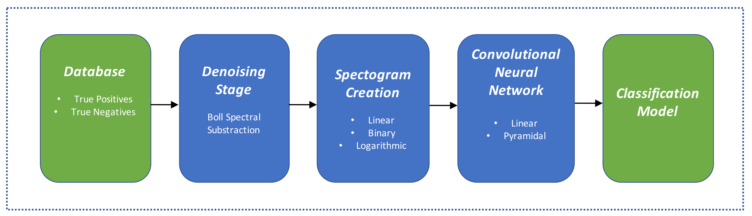
A scheme of the proposed analysis methodology used in this article is shown Figure 1. This research extends previous work from the authors presented in [5] by focusing in the denoising, spectrogram creation and classification aspects.

2.1. Data Source

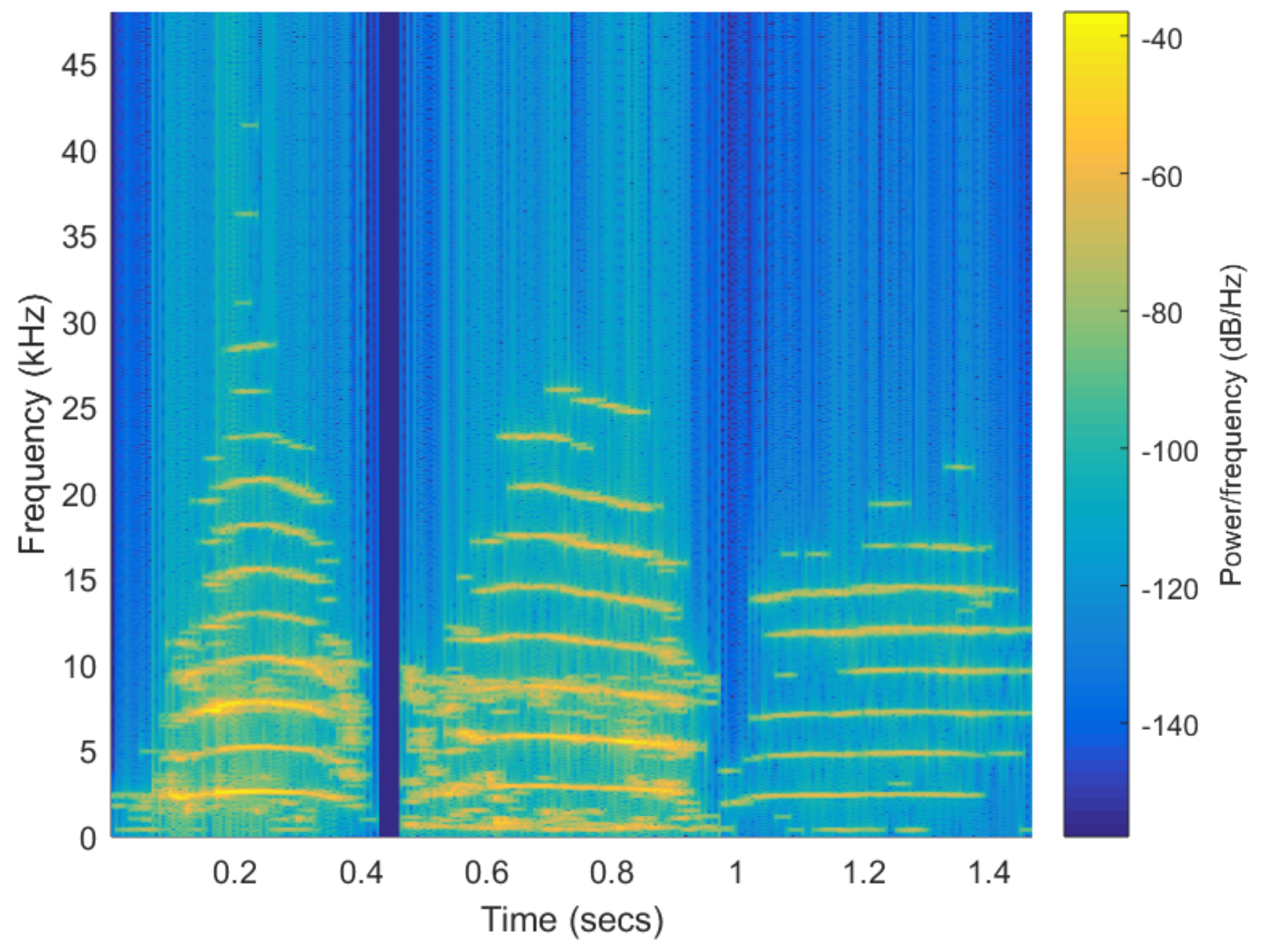
As described in [5] manatee vocalizations consist of single-note calls with several harmonics with frequency modulation, overtones and other nonlinear elements. For Antillean manatees recorded in Panama wetlands, the average fundamental frequency is around 3 kHz with a range between 0.7 and 8.1 kHz, and average duration is 362 ms with high variability (± 114 ms). Harmonic components typically reach around 20 kHz. Examples of vocalizations are shown in Figure 2.

Three databases were used in this study, prepared from audio clips recorded on the permanent monitoring sites in Changuinola and San San rivers, using Wildlife Acoustics SM3M bioacoustics programmable recorders (Maynard, MA, USA), placed 1 m above river floor at 2–3 depth. A detailed map of the river localizations and the surroundings is shown in Figure 3. The sampling frequency of the recorders was set at 96 kHz.

The first database included 507 curated manatee vocalizations and 177 sounds of the habitat (including noises produced by other species that co-exist in the habitat such as frogs and snapping shrimps, and low frequencies noises produced by currents and waves hitting the hydrophone unit). These sounds were obtained from audio clips recorded on two of the permanent monitoring sites (Figure 3), one in the Changuinola River (S1) and one in San San River (S3). The vocalizations and noise sounds were extracted from 65 (2-min) audio clips recorded from 1 May to 7 May 2018 from the Changuinola River and 62 (2-min) audio clips recorded from 7 July to 21 July 2017 from the San San River.

The vocalizations (positive samples) and noise sounds (negative samples) correspond to the true positive and false positive outputs, respectively, of the detection stage presented in [5]. This detection stage was based on the analysis of the autocorrelation of the signals in the wavelet domain using a mean-based threshold in each level. From the Changuinola River 313, and 128, true positives and false positive signals were detected in the audio clips, respectively. In the River San San, 194 true positives and 49 false positive signals were detected. It is noteworthy that vocalizations in this database presented a low SNR affected by background noise or other interferences. Some vocalizations only presented one harmonic component or were degraded. Thus, this database represents signals with the regular field acquisition conditions.

The second database, consisting of an additional new set of 166 noises (negative samples), were obtained from the same audio files using a more sensitive threshold (i.e., median-based threshold) in the detection stage. This set was prepared to be able to achieve class balance in some of the proposed experiments (see Section 2.4).

The third database included a set of 200 vocalizations from 20 different manatees (10 vocalizations per manatee). This database was prepared by visually inspecting spectrograms in the recordings of 20 days with the greater number of vocalizations determined by using the detection stage proposed in [5], in the whole data set of audio clips, from April 2015 to May 2018, and from the four permanent monitoring sites. This preparation process entailed the search of vocalizations with the same features in each day to have a group of vocalizations generated, likely, by the same individual. This database generally presented vocalizations with a higher SNR or quality that the first database.

Each element of the databases consists of short audio clips with a duration between 70 ms to 800 ms.

2.2. Spectrogram Generation

Before generating spectrograms all signals were denoised using Boll’s spectral subtraction method [41] to minimize the presence of noise or unwanted artifacts in signals where vocalizations were present. This denoising method had a significantly lower computational cost that the signal subspace approach used previously [5].

To generate the spectrograms, the FFT-based short-time Fourier transform with 50% overlapping windows of 1024 samples was used. This size of window provided a good compromise between temporal and frequency resolution for the sampling frequency of 96 kHz. Regardless of the duration of each signal, they were zero-padded and centered to obtain spectrograms with a fixed image size of 257 × 150 pixels to achieve dataset homogeneity.

Three formats to represent the amplitude in the spectrogram were considered: (1) binary, (2) linear and (3) logarithmic. To generate the binary representations, a threshold was set based on a selected value proportional to the amplitude mean of each signal spectrogram. To enhance the harmonic profiles, morphological operators such are dilation and erosion were applied. For both linear and logarithmic representations, the scale of the values represented on each spectrogram were calculated in relation to the maximum value recorded, that is, the representations were normalized on a linear and logarithmic scale, respectively.

2.3. Convolutional Neural Network Model Setup

For this task, it was determined that testing should be performed on two different feed-forward CNNs, a fixed filter size that we named the linear architecture (akin to bulbul architecture from Grill et al. [39]), and one with an increasing filter size that we named the pyramidal architecture (akin to the network describe in Bermant et al. [40]). Both architectures share similar architectures in terms of the placement of the convolutional, pooling and dense layers, only differing in the filter size of the kernels. The models, whose specific layers and dimensions are shown in

Table 1. Structure of linear and pyramidal network architectures.

Linear Architecture			Pyramidal Architecture
Layer	Filter	Kernel Size	Layer	Filter	Kernel Size
Conv2D	32	3 × 3	Conv2D	16	3 × 3
MaxPool	-	3 × 3	MaxPool	-	3 × 3
Conv2D	32	3 × 3	Conv2D	32	3 × 3
MaxPool	-	3 × 3	MaxPool	-	3 × 3
Conv2D	32	3 × 3	Conv2D	64	3 × 3
MaxPool	-	3 × 3	MaxPool	-	3 × 3
Fully Connected Layers			Fully Connected Layers
Dense	256		Dense	256
Dense	32		Dense	32
Dense	1		Dense	1

, were built using the Keras library [42]. A brief description and characteristics of each architecture can be detailed as follows:

(a)

Linear architecture: This network has a receptive field of 150 frames which are processed into a single binary output. It is composed of three sets of 32-filter convolutional and max pooling layers, which compress the input into 32 feature maps of 17 × 30 units. This output is then passed through three fully connected layers of 256, 32 and 1 unit which eventually classify the input. The ReLU activation function was used for every layer that required it except for the output layer which used the sigmoid activation function. The total number of parameters used by this network is 2,121,201.

(b)

Pyramidal architecture: This network also has a receptive field of 150 frames processed into a single binary output. It is composed of three sets of 64, 32 and 16-filter convolutional and max pooling layers, which compress the input into 16 feature maps of 17 × 30 units. This output is then passed through the same fully connected layers and activation functions as the previous model. The total number of parameters of this network is 4,205,249.

Training Parameters

The training for all networks was done over 50 epochs, feeding the network with 16 images per batch. For the stochastic gradient descent (SGD) optimizer, an epsilon of 1 × 10${}^{-8}$ and initial decay of 1 × 10${}^{-6}$ parameter for ADAM [43] updates were used with beta 1 of 0.9 and a beta 2 of 0.999 and a learning rate of 0.001. The Loss function was chosen to be binary cross-entropy (since were only interested in classifying vocalization and noise). Neuron dropout rate was set to be 50% after each epoch.

All the calculations regarding spectrogram representations and experiments were carried out in a personal computer with an Intel Core i7-6700HQ 2.6 GHz of CPU, with 8 GB of DDR4-2400 RAM on 64 bit and NVIDIA Geforce GTX 1060 GPU card with 6 GB of RAM.

2.4. Experimental Setup

Six experiments were devised to test the limits of detection of the manatee vocalizations, as follows:

(a)

Experiment #1—end-to-end training with different representations and architectures: The objective of this experiment was to find the best combination of spectrogram representation (binary, linear and logarithmic) and network architecture (linear and pyramidal, with and without dropout). For this experiment the first database, described in Section 2.1 was used. This database consisted of 441 manatee vocalizations (positive samples) and 177 noises (negative samples).

To assess the time performance of each network architecture and representation combination, a on_train_begin callback was set as global measurement of experiment start for counting all times. Also, a self.time function call was defined to measure time elapsed for any interval of interest, such as: on_test_begin, on_test_end, on_epoch_begin and on_epoch_end. For instance, training times were defined as the subtraction of the complete epoch times minus the test time, and the test times were calculated directly. The cumulative training time was the sum of each consecutive training time, which unlike individually recorded training times, was not reset after every epoch. All time calculations were made subtracting the time differences for each interval of interest, and were consequently added to a predefined list, for which sums and averages were calculated.

(b)

Experiment #2—analyzing the impact of training and testing data with K-fold cross-validation: The objective of this experiment was to find not only the best architecture, but the best testing/training vocalization combination. To test this, a 5-fold cross-validation is done with groups divided randomly with 80% used for training and 20% used for testing purposes. This experiment uses the same database as Experiment #1.

(c)

Experiment #3—analyzing the impact of training and testing data with selected clusters of vocalizations: The objective of this experiment is to better understand the model in the presence of a controlled database of the positive and negative classes. For this experiment the positives samples corresponded to the third database described in Section 2.1 (i.e., 200 vocalizations from 20 different individual manatees, 10 vocalizations each). The negatives samples corresponded to the 177 negatives samples of the first database. It is noteworthy that the training and validation partitions were arranged in such way that vocalizations of 16 manatees were used for training and vocalizations of 4 manatees were used for validation. Vocalizations of the same manatee were not in both partitions.

(d)

Experiment #4—prediction with models trained with regular SNR vocalizations: The objective of this test was to assess the limits of the prediction of the trained model using the positive samples collected regularly in the rivers (i.e., first database) and tested on a database with positives samples of selected good quality (i.e., high SNR signals) manatee vocalizations (i.e., third database). It should be mentioned that the training set presented some low SNR or degraded vocalizations. To keep class balance, for the training process 200 positives samples were used from the first database and 200 negatives samples from the second and third database. For the prediction test, 140 positives samples of the third databases, combined with 140 (different) samples of the first and third database were used.

(e)

Experiment #5—prediction with model trained with high SNR vocalizations: In this experiment, the databases used for training and prediction in experiment #4 were exchanged. The objective was to test how a model trained with high SNR signals will perform in a set of regularly recorded positive samples from the rivers. Thus, in the training process 200 positives samples from the third database and 200 negatives samples from the firsts and second databases were used. For the prediction test, 140 positives samples of the first database and 140 negatives samples of the first and second database were used.

(f)

Experiment #6—comparative study between the CNN approach and the signal processing FFT-based harmonic search approach: In this experiment the proposed CNN architectures and the modified Niezrecki harmonic method presented in [5] were used to classify signals (i.e., prediction) on the databases of the Changuinola and San San rivers.

The network used to predict on the Changuinola River was trained with 194 positive samples of San San River (first database) and 42 positive signals from 14 different manatees (3 samples per manatee) of the third database, for a total of 236 positive samples. A total of 194 negatives samples were used to train the networks, 49 negative samples of San San River (first database) and 145 negative samples from the third database. The networks used in San San River were trained using a total of 355 positive samples (313 from Changuinola River and 42 from the third database) and a total of 294 negative samples (128 from Changuinola River and 166 from second database). The goal of adding positive samples from the third database was to increase the vocalization diversity for each training set.

The signal processing method consisted in the search of harmonic components in the FFT spectrum of 3 segments of the signal under analysis: one segment near the beginning of the signal, one on the center and one segment near the end [5]. The search implies the verification of the presence of two or more harmonic components and the absence of components between those components (or valleys). The method also considered the special case of vocalizations with only one harmonic component. The method presented three operation modes, as follows: Operation mode #1 requires that only 1 segment verifies the required criteria. For operations modes #2 and #3, it is required that the criteria are verified in segments 2 and 3, respectively. Operation modes allow the ability to adjust the precision and recall metrics of the method according to the application requirements, operation mode #1 being the one with the smallest precision and the highest recall, and operation #3 being the one with the greater precision and smaller recall. Operation mode #2 presented intermediate values of precision and recall. The signal processing method does not require training. However, it required that the user empirically adjust several thresholds to detect harmonics and valleys in the FFT-spectrum of the signal.

It is noteworthy that the rivers present different noise conditions. The Changuinola River consist of sinuous narrow (<20 m) channels with abundant surface and subaquatic vegetation. In the other hand, the San San river is wider (>50 m) and has less vegetation. In consequence, Changuinola River audio clips present more background noise than those from San San River.

Classification Metrics

For the experiments described above, metrics for the evaluation of their classification performance were used.

Table 2. Theoretical confusion matrix between actual and predicted classes.

		Actual
		Positive	Negative
Prediction	Positive	TP	FP
	Negative	FN	TN

shows the confusion matrix for a general binary classification experiment. The performance of the model was related to the capacity to provide true predictions: true positive (TP) and true negative (TN), it was also accounted for prediction errors or false prediction: false positive (FP) and false negative (FN).

From the confusion matrix and the relation between (TP, FP, TN and FN) a five metrics can be determined, described hereafter:

• Accuracy: used to evaluate the number of true predictions made by the model, calculated with the following formula: $\frac{\#TP+\#TN}{\#TP+\#TN+\#FP+\#FN}$.
• Precision: used to evaluate the proportion of positive predictions that were correctly classified, it is also called positive predictive value (PPV) and is calculated using the formula $\frac{\#TP}{\#TP+\#FP}$.
• Recall: used to evaluate what proportion of the actual (observed) positive predictions that were correctly classified, it is also called sensitivity or true positive rate (TPR) and is calculated using the formula: $\frac{\#TP}{\#TP+\#FN}$.
• F1 Score: used to evaluate the model accuracy, considering both the precision and recall. It ranges from 0 (worst) to 1 (best, perfect precision and recall). It is often used when there is class imbalances in the data set, is calculated using the formula: $2\ast \frac{Precision\ast Recall}{Precision+Recall}$.
• Area Under the Receiver Operator Characteristics Curve (AUROC): is a graph used to evaluate the performance of a model at different thresholds of classification, usually allowing a greater number of positive predictions at at lower thresholds, thus increasing both false positives and true positive. The Receiver Operator Characteristics (ROC) curve is used to show two parameters: the true positive rate (TRP or recall) and the false positive rate (FPR) using the formula $\frac{\#FP}{\#FP+\#TN}$.

2.5. Visualizing Trained Features of the Network

One of the main questions that arises with the use of CNN for classifications of images is to understand what is the model actually learning. To solve this problem Zeiler and Fergus in [44], proposed the technique of projecting the feature activations back to the input pixel space, that is, to reconstruct an image and to explore the evolution of features along the training phase in each layer to be able to determine any representation problem that might arise in the network. Mahendran and Vedaldi on [45] applied the method of inversion of images and applied to CNNs, further describing the fact that information in the layers becomes more and more abstract, however invariant to the original image.

This technique of reconstructing intermediate interpretations has been of great importance in the medical fields, helping clinicians to visualize what CNN models learn in their respective domains. As an example, in [46] the authors present the visualization of intermediate representations in the context of detection of pneumonia and describe regions of interest in the differentiation between bacterial and viral types in chest X-ray (CXR).

To further understand what features of the vocalizations the model was actually learning, intermediate layer reconstructions were made for the model in Experiment #3, and analyzed accordingly.

3. Results and Discussion

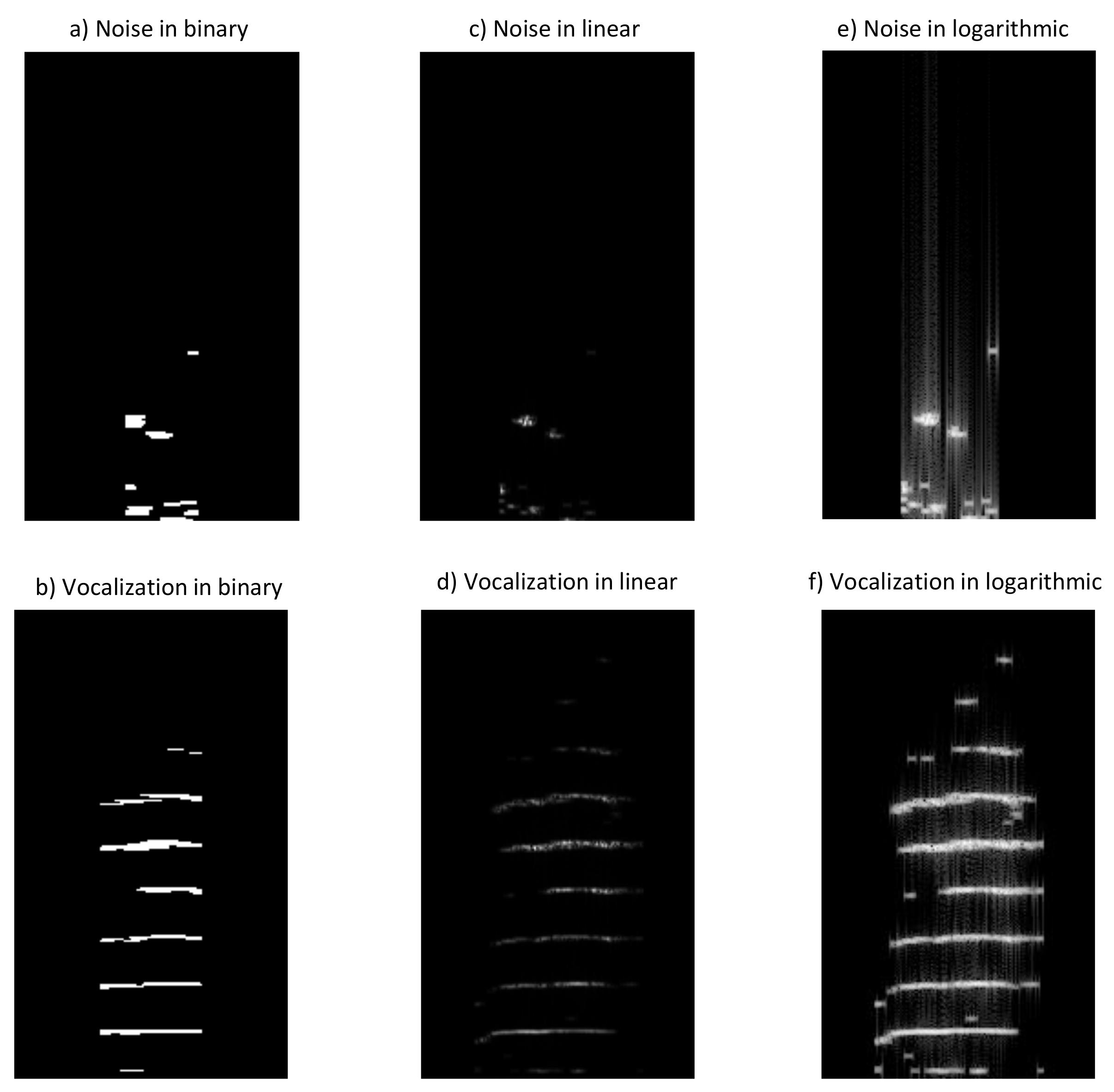
After structuring the vocalizations defined in Section 2.1, spectrograms representations were created using the methods previously described in Section 2.2 (binary, linear and logarithmic), for both negative (noise) and positive vocalizations. Resulting spectrograms for both classes can be seen in Figure 4, respectively. Resulting images suggest that of the three representation methods tested, binary spectrograms seem to have a better contrast, showing clearer lines and harmonics.

3.1. Results for Experiment #1—End-to-End Training with Different Representations and Architectures

Table 3. Results for Experiment #1 end-to-end training with different spectrogram representations and networks architectures.

Spectrogram Type	Network Architecture	Accuracy	Loss	Val. Accuracy	Val. Loss
Binary	Linear	100	3.79 × 10${}^{-4}$	96.35	0.5023
	Pyramidal	100	7.93 × 10${}^{-4}$	98.54	0.6116
	Linear w/Dropout	96.53	0.0906	94.16	0.2677
	Pyramidal w/Dropout	97.99	0.0542	94.16	0.1555
Linear	Linear	100	1.38 × 10${}^{-5}$	98.54	0.4383
	Pyramidal	100	2.48 × 10${}^{-4}$	98.54	0.4216
	Linear w/Dropout	99.09	0.0311	97.81	0.3838
	Pyramidal w/Dropout	99.13	0.022	97.81	0.9781
Logarithmic	Linear	100	1.95 × 10${}^{-4}$	97.08	0.162
	Pyramidal	99.27	0.02	93.43	0.9343
	Linear w/Dropout	95.98	0.1316	98.54	0.041
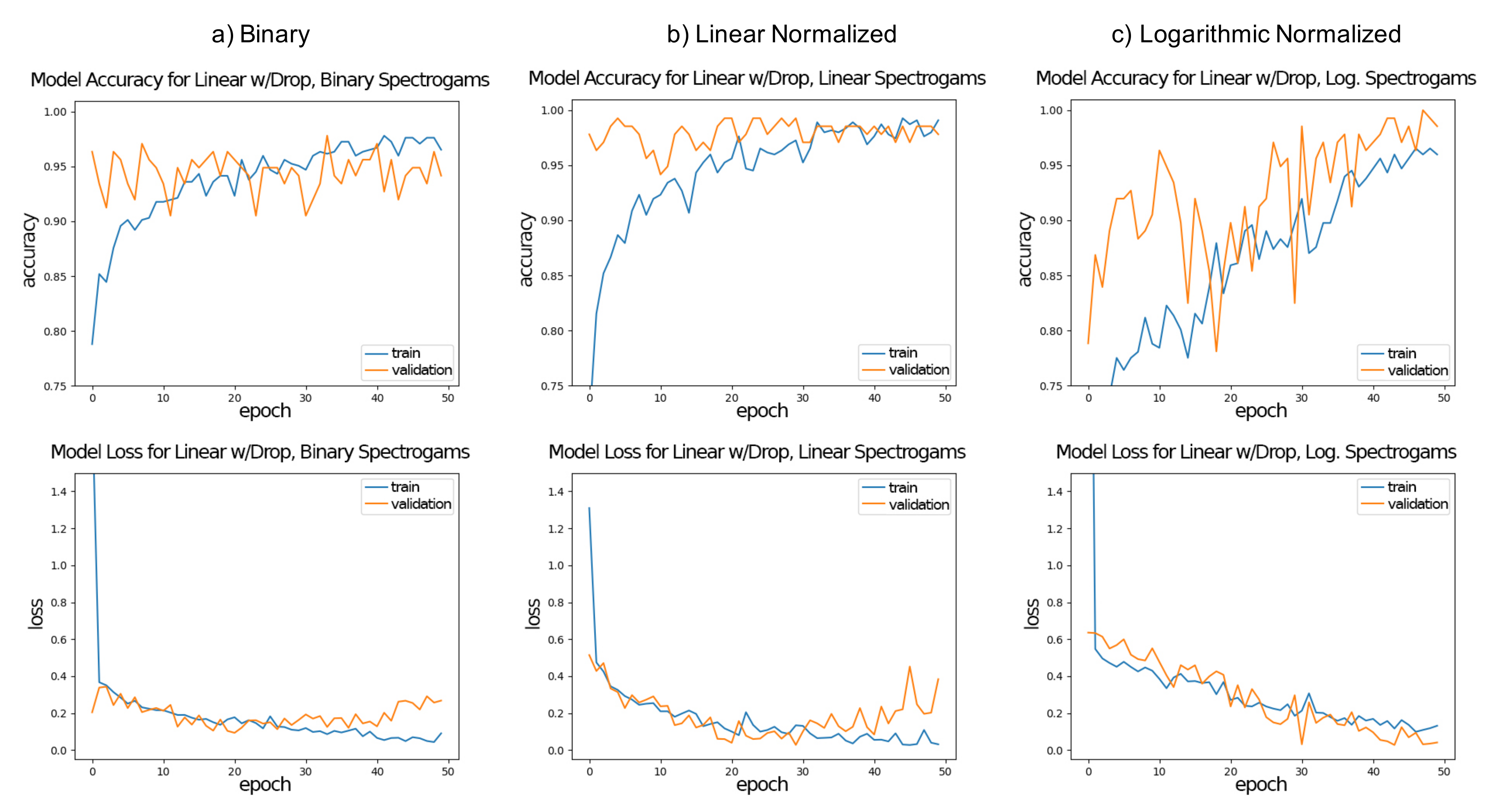
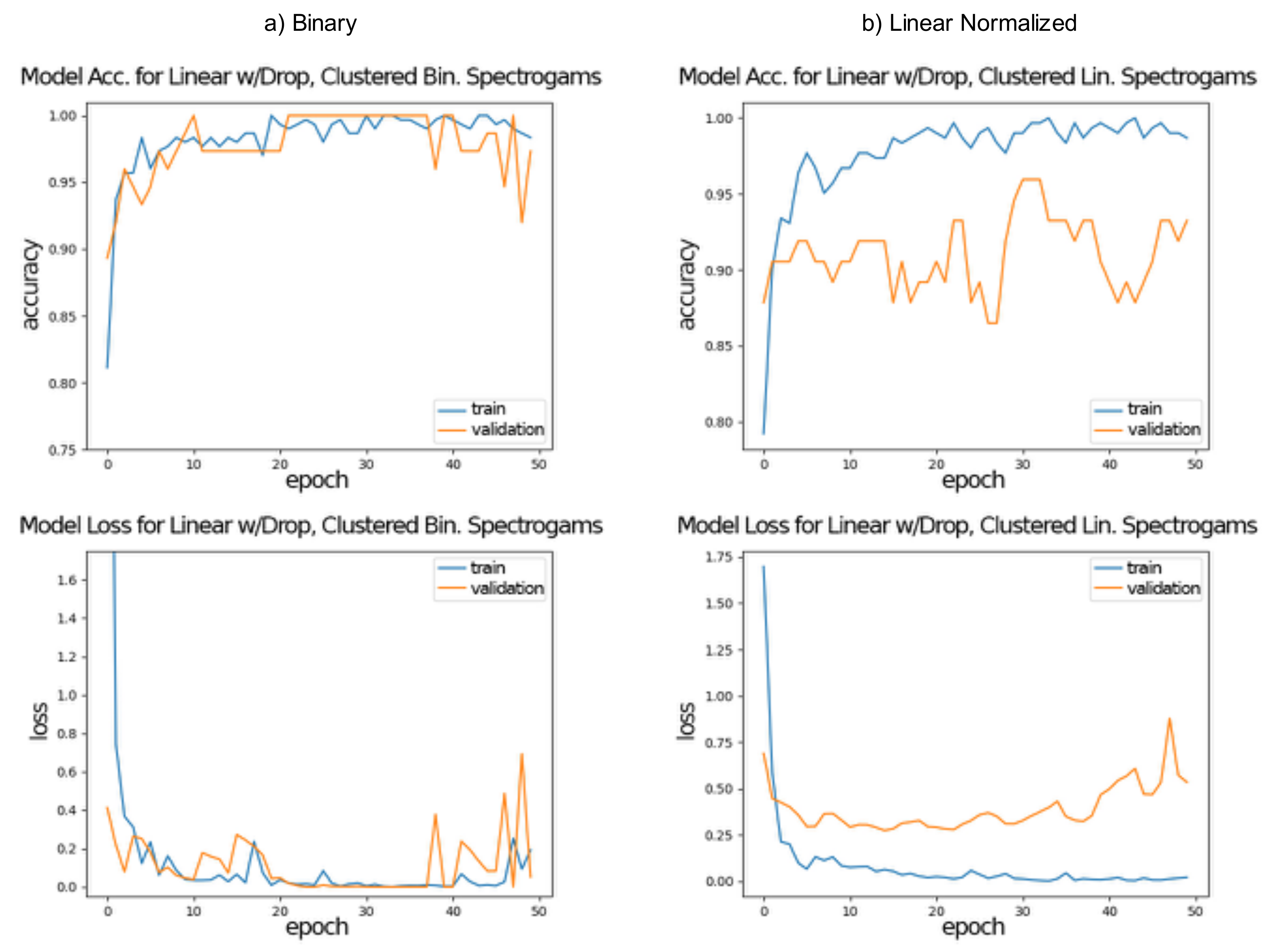
	Pyramidal w/Dropout	94.33	0.1488	98.54	0.0294

shows the results for training and testing, both in the accuracy and loss values for each representation/network architecture combination. All models were suitable for the classification task, with no combination having a striking different result. In terms of accuracy all models were able to achieve over 94% results after 50 epochs for the testing set, with a few 100% for the linear spectrogram representation. A similar value of over 94% was achieved for the validation set. In terms of the loss function, resulting errors were less the 0.1 for testing and were below 1.00 for the validation set. Accuracy and loss curves for linear with dropout architecture for (a) binary, (b) linear normalized and (c) logarithmic normalized spectrogram representations are shown in Figure 5.

The time performances of the architectures and representation combinations are shown in

Table 4. Time performance for Experiment #1, for the complete training and inference task and average per epoch.

		Time (s)
		All Epochs		Per Epoch
Spectrogram Type	Network Architecture	Training	Inference	Avg. Training	Avg. Inference
Binarized	Linear	716.03	34.06	14.32	0.69
	Pyramidal	633.75	27.19	12.67	0.54
	Linear w/Dropout	824.87	34.37	16.49	0.68
	Pyramidal w/Dropout	713.55	27.07	14.27	0.54
Linear	Linear	717.87	34.21	14.36	0.68
	Pyramidal	640.81	27.13	12.81	0.54
	Linear w/Dropout	827.55	34.29	16.55	0.68
	Pyramidal w/Dropout	714.59	27.38	14.29	0.54
Logarithmic	Linear	725.35	34.53	14.51	0.69
	Pyramidal	640.88	27.3	12.81	0.55
	Linear w/Dropout	833.33	34.26	16.66	0.68
	Pyramidal w/Dropout	720.76	27.44	14.41	0.54

. As expected, the training time was higher than the time spent in doing the inference. This behavior was seen on both the time for all epochs and the time per epoch. More importantly for our assessment, regardless of the spectrogram type, the linear architecture consumed longer computational time than the pyramidal architecture. Even when the dropout rate was fixed at 50%, it added over 100 s for the complete training, which translate to roughly 2 s per epoch.

3.2. Results for Experiment #2—K-Fold Validation

Table 5. Results for Experiment #2, end-to-end training with different spectrogram representations and networks architectures with five-fold cross-validation.

		Testing Accuracy per Fold
Spectrogram Type	Network Architecture	Fold #1	Fold #2	Fold #3	Fold #4	Fold #5	Mean ± Stdev
Binary	Linear	92.7	86.86	91.24	89.78	88.97	89.91 ± 1.99
	Pyramidal	91.24	87.59	91.24	86.13	88.24	88.89 ± 2.04
	Linear w/Dropout	89.78	84.67	89.78	88.32	89.71	88.45 ± 1.97
	Pyramidal w/Dropout	90.51	85.4	90.51	94.89	88.24	89.91 ± 3.12
Linear	Linear	93.43	94.43	94.89	91.97	92.65	93.27 ± 0.98
	Pyramidal	94.16	92.7	96.35	93.43	91.91	93.71 ± 1.52
	Linear w/Dropout	95.62	96.35	94.16	92.7	93.38	94.44 ± 1.36
	Pyramidal w/Dropout	94.16	91.97	89.78	91.97	93.38	92.25 ± 1.50
Logarithmic	Linear	87.59	90.51	85.4	90.51	92.65	89.33 ± 2.54
	Pyramidal	89.78	92.7	90.51	86.13	93.38	90.50 ± 2.56
	Linear w/Dropout	91.24	94.16	72.26	93.43	93.38	88.90 ± 8.37
	Pyramidal w/Dropout	92.7	91.24	89.78	90.51	94.85	91.82 ± 1.80

shows the resulting accuracy from the five-fold variation on every model/representation after 50 epochs, also the mean and standard deviation for every model/representation was also calculated. Results suggest that the linear representation and a linear model with dropout was the best for classifying true negative and positive vocalizations with a mean of over 92%, then, models using the logarithmic representation and at last, models using the binary representation. A partial cause for this can be that in logarithmic representations the presence of background noise and other interferences are enhanced in the positive vocalizations (i.e., applying the logarithm function on the spectrogram enhances low amplitude signals), resulting in it being more difficult to distinguish negative (noise) samples from positive vocalizations.

A preliminary conclusion of Experiments #1 and #2 was that CNNs can be applied for the analysis of vocalization in classification tasks, with an accuracy of close to 94%, even in the validation set. However, after a detailed analysis on results for the validation set of Experiment #1 for linear with dropout architecture, shown in Figure 5, we realized that the improvement of the percentage of accuracy stopped early, which was an indication of over-fitting, especially for the binary and logarithmic normalized spectrogram representations. There are a few reasons for this, maybe due to the fact that a limit was reached in the capabilities of the model. Indeed, Experiment #2 was designed to be a five-fold cross-validation, therefore to avoid over-fitting of the model, and results showed better validation accuracy for all cases.

3.3. Results for Experiment #3—Analysis of Clusters of Vocalizations

Table 6. Results for Experiment #3, analyzing the impact of data set from different cluster of vocalizations.

Spectrogram Type	Network Architecture	Accuracy	Loss	Val. Accuracy	Val. Loss
Binary	Linear w/Dropout	98.34	0.1923	97.33	0.0514
	Pyramidal w/Dropout	99.01	0.0097	93.33	0.2481
Linear	Linear w/Dropout	98.68	0.0211	93.24	0.5342
	Pyramidal w/Dropout	95.71	0.0499	91.89	0.9218

shows the resulting accuracy and loss for training and testing for both binary and linear representation with linear and pyramidal network architectures with dropout. As can be seen in Figure 6, after 50 epochs, results showed that binary representation with a linear architecture with dropout was the best model for classifying vocalizations coming from four (4) manatees not previously seen by the model (not part of the training database) and used validation achieving over 98% in testing and over 97% in validation accuracy.

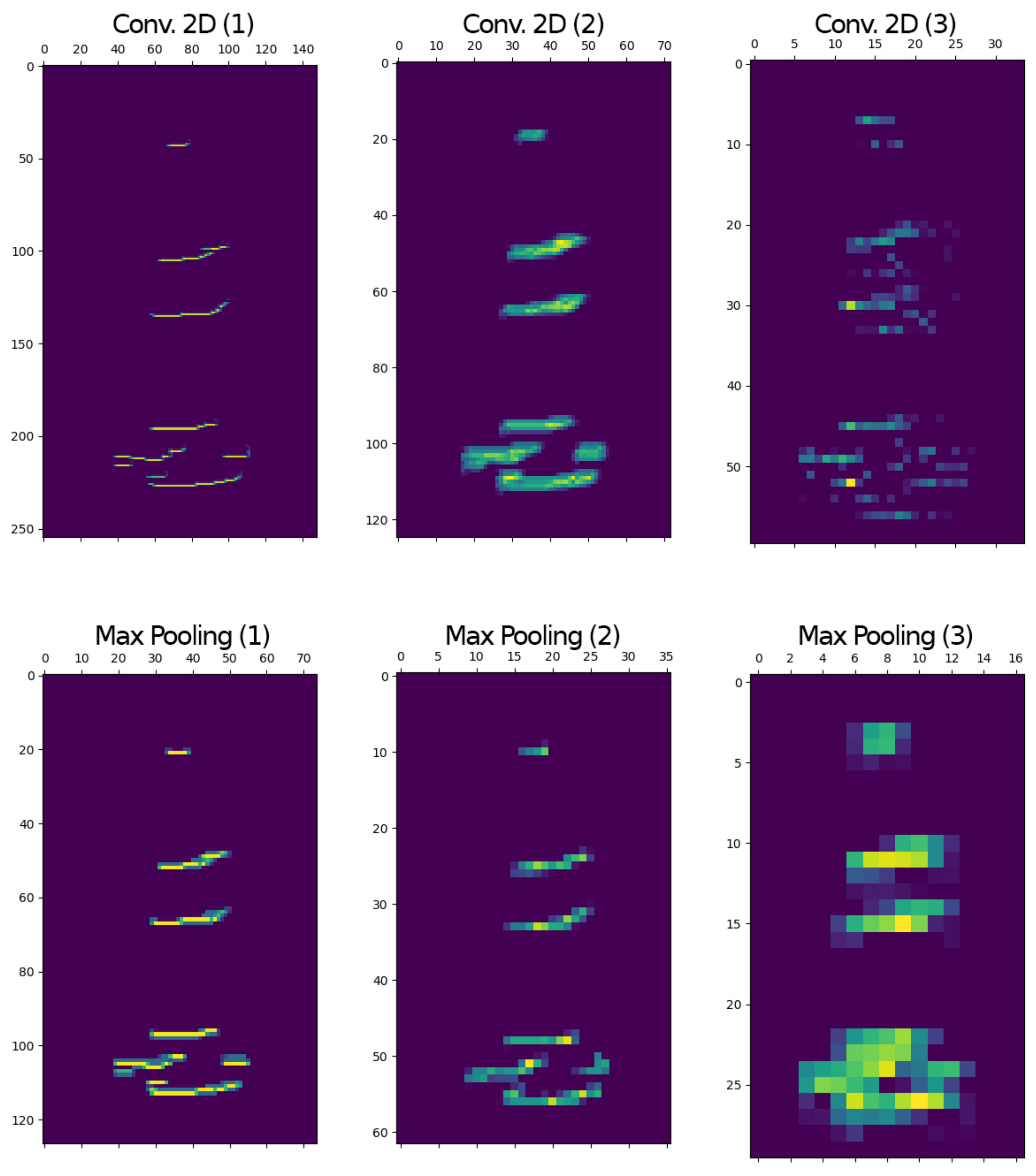
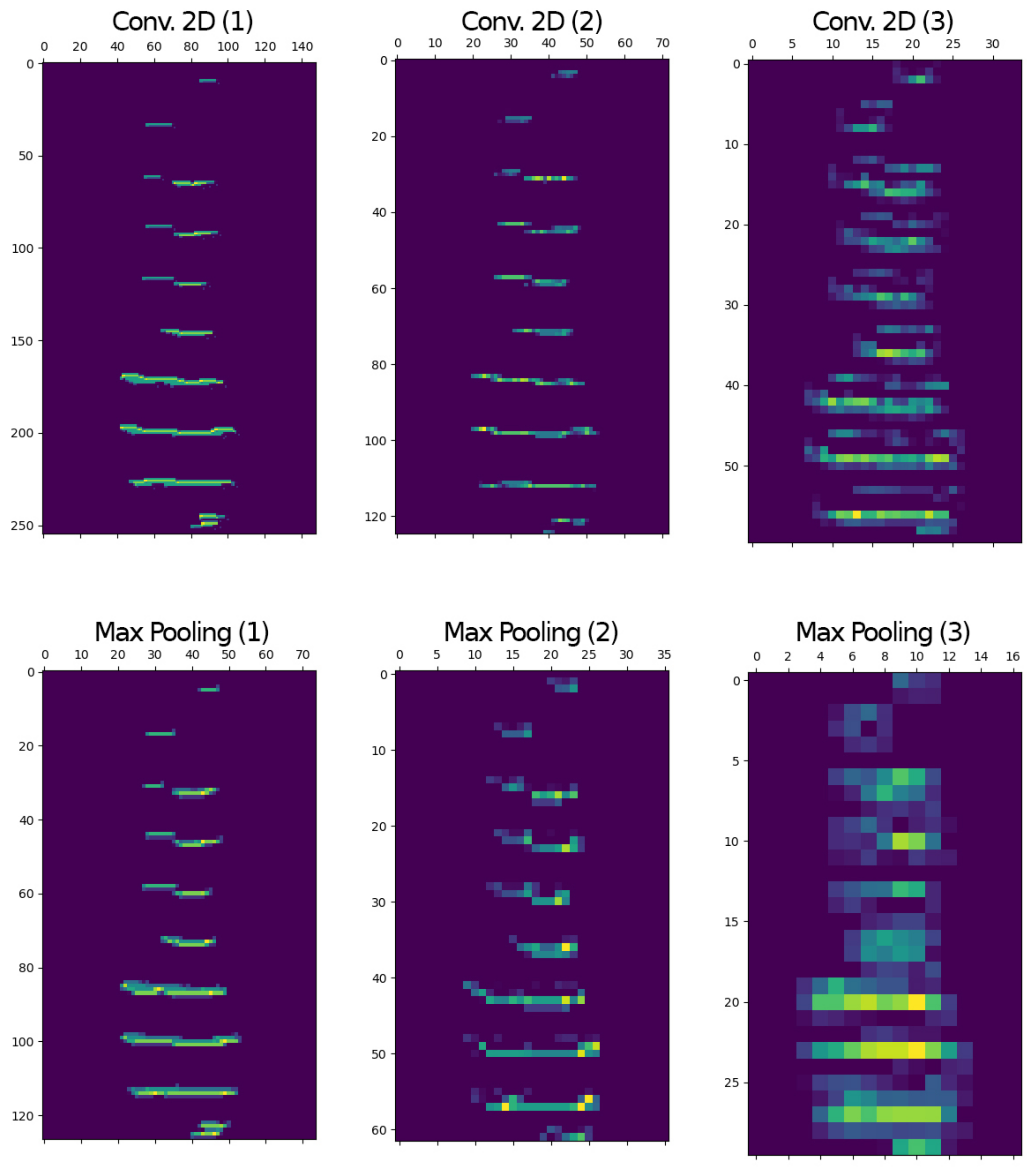
When looking at the intermediate representations of the activations of one channel, that is, one image per convolutional layer (see Figure 7 and Figure 8), it was evident that the linear architecture with dropout was effectively learning the shape of the vocalizations in binary and linear representations, respectively.

3.4. Results for Experiments #4 and #5—Predicting Vocalization Class

Results for Experiment #4 and Experiment #5 are presented in

Table 7. Results for Experiment #4 and #5 on different metrics of classification assessment.

		Experiment #4				Experiment #5
Spectrogram Type	Network Architecture	AUC	Precision	Recall	F1	AUC	Precision	Recall	F1
Binary	Linear w/Dropout	0.954	0.98	0.93	0.902	0.864	0.921	0.585	0.715
	Pyramidal w/Dropout	0.951	0.94	0.89	0.91	0.876	0.872	0.65	0.744
Linear	Linear w/Dropout	0.908	0.95	0.81	0.87	0.912	0.958	0.465	0.626
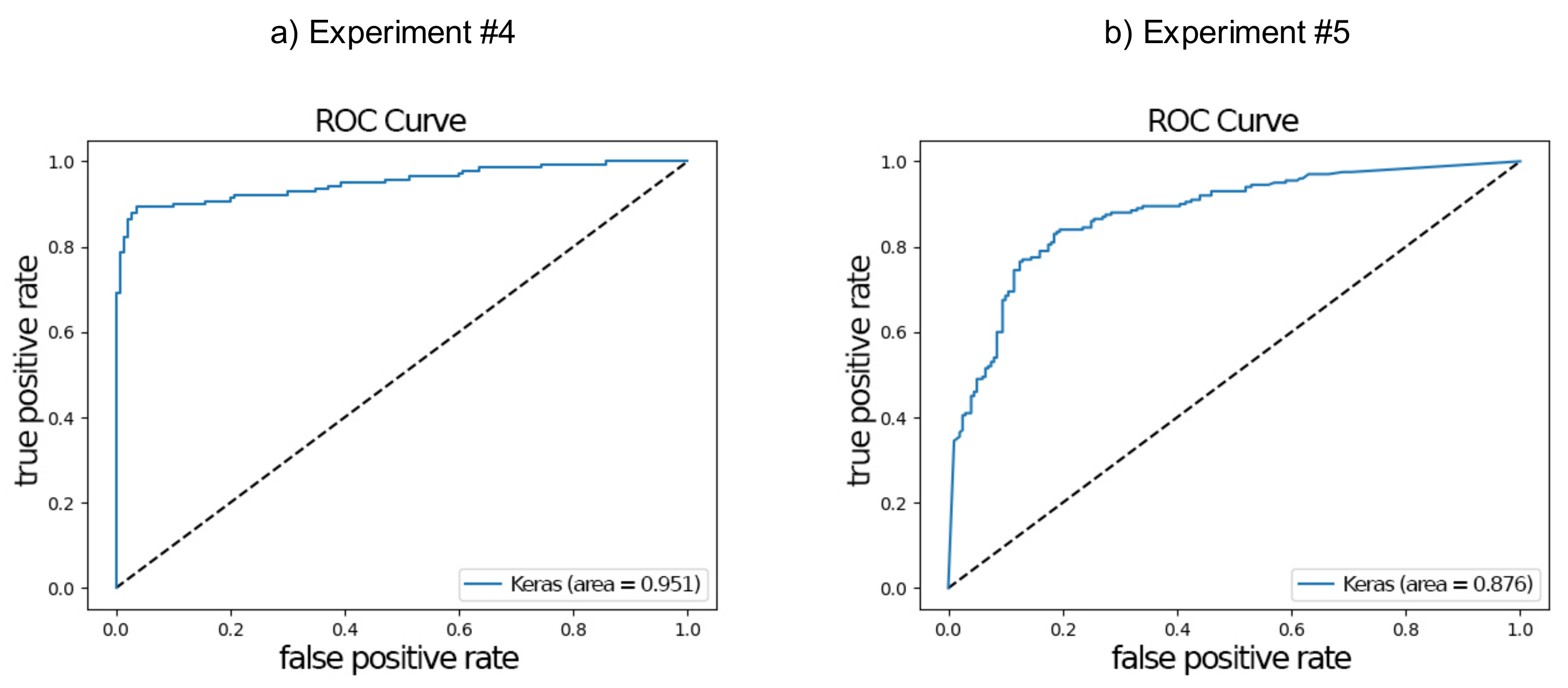
	Pyramidal w/Dropout	0.927	0.92	0.85	0.88	0.849	0.944	0.505	0.657

, showing that the model trained using regular recorded signals from the rivers (Experiment #4) was able to provide accuracy and precision over 0.92 for both binary and lineal representations. Recall and F1 scores obtained for both representations were over 0.81 and 0.87 for both representations, with the binary representation reaching the highest values (0.93 and 0.91, for the lineal and pyramidal architecture, respectively). Overall, the binary representation provided the highest performance for all these metrics. Moreover, the model trained using mostly high SNR signals from 20 different manatees (Experiment #5) provides lower performance than the model trained using regular signals recorded from the rivers. In particular, the obtained recall for the binary and linear representations were 0.65 and 0.50 for the pyramidal architecture and 0.585 and 0.465 for the linear architecture, respectively, which was significantly lower than the previous model (Experiment #4). This could be explained by the fact that the training database did not have low SNR or degraded signals that leads to a higher number of false negatives (i.e., lower number of true positives).

Figure 9 shows the ROC curves for binary representation for pyramidal with dropout architecture for both Experiment #4 and Experiment #5. The curve on Figure 9a shows better results than the curve on Figure 9b, which was also evident by the area under the curve of 0.95 and 0.88, respectively. This combination of spectrogram type (binary) and architecture (pyramidal with dropout) provided the best performance for both experiments in terms of F1 score.

3.5. Results for Experiment #6—Comparing the CNN-Based and Signal Processing-Based Approaches

The performance of the CNN networks and the FFT-based harmonic search methods are presented in

Table 8. Results for Experiment #6 for the convolutional neural network (CNN) approach on different metrics of classification assessment.

			Metrics
River	Spectrogram Type	Model	AUC	Precision	Recall	F1
Changuinola	Binary	Linear w/Dropout	0.905	0.930	0.856	0.891
		Pyramidal w/Dropout	0.901	0.931	0.738	0.823
	Linear	Linear w/Dropout	0.902	0.967	0.671	0.792
		Pyramidal w/Dropout	0.904	0.961	0.702	0.811
San San	Binary	Linear w/Dropout	0.858	0.908	0.871	0.889
		Pyramidal w/Dropout	0.858	0.887	0.896	0.892
	Linear	Linear w/Dropout	0.899	0.902	0.907	0.904
		Pyramidal w/Dropout	0.919	0.934	0.886	0.910

and

Table 9. Results for Experiment #6 for the modified Niezrecki approach on different metrics of classification assessment.

		Metrics
River	Mode	AUC	Precision	Recall	F1
Changuinola	1	0.738	0.799	0.840	0.819
	2	0.734	0.930	0.674	0.781
	3	0.589	0.992	0.422	0.592
San San	1	0.790	0.815	0.954	0.879
	2	0.778	0.861	0.861	0.861
	3	0.609	0.923	0.557	0.695

, respectively. The CNN approach presented the higher accuracy and F1 scores than the harmonic search method for each river (Accuracy: 0.905 for Changuinola River and 0.919 for San San River; F1 Scores: 0.891 for Changuinola River and 0.889 for San San River).

The greatest precision values for both rivers were obtained by the harmonic search method on operation mode # 3 (0.992 for Changuinola River and 0.923 in San San River). However, for those cases the recall scores were very small (0.422 for Changuinola River and 0.557 for San San River). In general, the CNN approach present better scores for the harmonic search approach with a greater accuracy and greater balance between precision and recall (F1 Score).

CNN combinations of spectrogram types and architectures provided no strikingly different results, with the exception of the linear spectrograms in the Changuinola River which provided significantly smaller recalls (and F1 Scores). This may be explained by the presence of noise background and interferences with more power in this river and the fact that those networks were trained with San San River samples that did not have such noisy conditions. For this river, the effect of noise was less present in the binarized spectrogram, since the thresholding process eliminates most noise components from the spectrogram. In the case of Changuinola River, it would be of interest to do further testing using a training database from the same river with the same noise conditions.

Concerning the computational complexity, the harmonic search method implied the computation of three FFT of size $N=8192$ for this implementation. Each FFT required $\mathcal{O}(NlogN)$ operations. Other steps in this method as finding maximum values of a vector and comparisons of vectors required $\mathcal{O}\left(N\right)$ operations.

4. Conclusions

Automatic classification of sounds has progressed greatly with the use of convolutional neural networks. Despite the variance problem when representing sounds as spectrograms, CNNs are a suitable method for learning features relative for the classification tasks. In this work we used three types of spectrogram representations and explored two network architectures (with and without dropout), to assess the limits of classifications of negative (noise) and positive manatee vocalizations. Six experiments were devised to assess the behavior of these combinations with databases containing vocalizations and noises from two different rivers, San San and Changuinola in Bocas del Toro, Panama.

Results on the use of spectrograms suggest that they are a great way to be able to classify manatee vocalizations. However, based on our results a few conclusions can be made about spectrograms. It seems that one reason why these experiments work is that the classifications are done between unstructured noise and well-structured vocalizations. That can be attributed to the fact that both our databases contain signals from a previous detection stage (described in detail in [5]), where vocalizations are identified and clipped into shorter signals, later padded and centered to have a fixed image size to be processed by the networks. Moreover, this is reflected in the class imbalance found for the positives vocalizations. Basically, the system places more attention in the elimination of negative (noise) vocalizations.

In this work, databases were balanced using a different vocalization set, as in Experiment #3. However, data augmentation (DA), a technique that helps this imbalance by adding an intermediate step for the creation of new spectrograms could be used. It works by using techniques such as: cropping, padding, horizontal flipping and rotations, from images from lower count classes to create enough images to have balanced classes. Data augmentation is now a staple method in CNN, which is known to improve the accuracy of the classification [47]. Specific to our data set, it can be used can bring negative vocalizations to comparative numbers with the positive vocalizations data set. It can be used also for the positive data set if it keeps the harmonic structures of vocalizations intact. In addition, to address this issue the Synthetic Minority Oversampling TEchnique (SMOTE) algorithm [48] can be used. It is an oversampling method, that helps reduce class imbalance by producing new synthetic samples or data points. Also it is known to together with DA [49], with latter being used in data-space while the former can be applied to work on the feature-space of the minority data set.

Experiment #6 showed that the CNN-based approach presented a better performance in terms of accuracy and F1 score that the FFT-based harmonic search method used in our previous work [5]. From these results, we can conclude that the binary representation presents more consistent results.

In reference to network architectures, both the linear and pyramidal architectures with dropout were suitable for classification tasks providing similar results, however the pyramidal architecture presented both a shorter training and inference time (Experiment #1), which could be of special interest for a real time embedded implementation to rapidly classify the vocalizations for further detection and counting of manatees.

The results obtained with the CNN approach, here presented, can be used in a comprehensive comparative study with the FFT-based harmonic search approach and a more traditional machine learning method (probably an SVM), to assess their validity and classification capacity. To do this properly, the three approaches should be implemented in the same architecture, programming language and using the same vocalization databases to truly evaluate the classifications metrics and computational time. Something that for now is not possible given the different programming languages and heterogeneous hardware architectures used for the executions of these algorithms for the analysis.

This work complements and improves previous works in the classification of manatee vocalizations in the context of manatee detection and and individual identification schemes, as presented in [5]. Moreover, together with a recently published article by Brady et al. [50], in which Floridian manatee vocalization are studied using classification and regression tree (CARTs) and cluster analysis, are few of the examples of using machine learning and deep learning applied to the classification of manatee vocalizations.

Finally, the value of this work is that it supports ongoing efforts to estimate the population size and distribution range of this endangered species at local and regional levels to improve and manage the protection of Antillean manatee populations and fragile wetland habitats.