Designing Audio Equalization Filters by Deep Neural Networks

Abstract

Audio equalization is an active research topic aiming at improving the audio quality of a loudspeaker system by correcting the overall frequency response using linear filters. The estimation of their coefficients is not an easy task, especially in binaural and multipoint scenarios, due to the contribution of multiple impulse responses to each listening point. This paper presents a deep learning approach for tuning filter coefficients employing three different neural networks architectures—the Multilayer Perceptron, the Convolutional Neural Network, and the Convolutional Autoencoder. Suitable loss functions are proposed for each architecture, and are formulated in terms of spectral Euclidean distance. The experiments were conducted in the automotive scenario, considering several loudspeakers and microphones. The obtained results show that deep learning techniques give superior performance compared to baseline methods, achieving almost flat magnitude frequency response.

1. Introduction

Listening environments are characterized by reflections and reverberations that can adversely affect listening [1] and attention [2], adding unwanted artifacts to the sound produced by an acoustic source. For this reason, audio equalization is needed in order to improve sound quality reproduction. Of particular interest is the car scenario, where people daily listen to music, radio programs or take hands-free phone calls. The audio quality in such an environment is very important, but is adversely affected by several factors, including the loudspeakers quality and the reflective materials inside the cabin. The impulse response at the listening position is characterized by the sum of multiple signals: those coming from the loudspeakers and their reflections. Furthermore, the loudspeakers impose their frequency response on the signal. The frequency response is thus colored and usually results in deep notches and peaks, that reduce the audio quality.

These issues are generally addressed by the design of linear filters [3] that are applied to the signal before being transduced by the loudspeakers. The filters are designed to improve the audio quality at specific listening positions by inverting the car impulse response. However, the task is challenging, as the existence of the inverse may not be guaranteed, and the complexity increases with the number of sources and microphones. A plethora of design techniques have been proposed in the past for room equalization [1], and some have been proposed, more specifically, for the car scenario. These are, generally, based on linear optimization and inversion algorithms. Considering the complexity of this task, however, novel design techniques may be applied in this context, relying on nonlinear methods such as evolutionary algorithms, machine learning and neural networks.

Since digital communication systems are subject to the multipath problem, that is, the sum of multiple reflections in a linear channel with multiple sources and receivers, it is worth investigating the literature for equalization techniques applied to this application field. Indeed, several novel techniques have been proposed for the design of equalizing filters for digital communications, relying on nonlinear methods. In Reference [4], the authors use Particle Swarm Optimization (PSO) to equalize the impulse response of an optical fiber communication. This is shown to provide better results than Least Mean Square (LMS) and Recursive Least Square (RLS) techniques. Another interesting PSO approach is reported in Reference [5], where the PSO particles are used to obtain optimal poles and zeros of an IIR filter. In Reference [6] Genetic Algorithms (GA) are exploited for Adaptive Channel Equalization, in order to reduce the Inter Symbol Interference (ISI) present in the trasmission channel.

Although inspiring, these algorithms cannot be employed in the audio equalization scenario, as the two tasks differ in several aspects. While in communication systems equalizers are implemented at the receiving end, in the audio case they can only be implemented at the sound source. This can represent an issue, as the equalizing filters must provide satisfying results at several listening positions, while with telecommunication devices, each one can adapt its equalizing filter depending on the incoming signal. In communication systems the main goal is reducing symbol error rate, thus, allowing a robust classification of the symbols constellation, while in the audio field the goal is to achieve near-perfect audio quality taking psychoacoustic factors into consideration. Finally, the communication scenario may or may not consider time-varying environmental conditions (e.g., mobile receiving stations), while in the audio field time-invariance is often assumed, thus, room impulse responses are measured and treated statically.

A first attempt at the use of deep learning for audio equalization is found in Reference [7], where the authors use a Time Delay Neural Network (TDNN) to solve the problem of equalization, using the input sequence, delayed by a time unit, as input and the signal recorded by the microphone as output: the error between the input signal and the output of the network is used for the back-propagation algorithm. The forward approach is also employed using a delayed copy of the input signal as input and the difference between the output given from the loudspeaker and the network as error. In References [8,9], the authors describe a system that maps the gain of each frequency band with the user’s preferred equalizer settings as training data. A similar approach is undertaken in Reference [10], where k-Nearest Neighbour (KNN) is used to implement a timbre equalizer based on user preference in terms of brightness, darkness and smoothness. Specifically, sound professionals and music students were asked to manually equalize 41 audio segments. Equalization for music production were performed in Reference [11], where a Dilated Residual Network (DRN) was used to automate the resonance equalization in music, predicting the optimal attenuation factor, while an end-to-end equalization was used in Reference [12], substituting filter banks with Convolutional Neural Network (CNN) and without prior knowledge of filter parameters, like gains, cut-off frequency and quality factor.

Recent works addressing the design of IIR filters using PSO can be found in References [13,14,15]. In particular, Foresi et al. [15] use PSO with fractional derivative constraints to design a quasi-linear phase IIR filter for Audio Crossover Systems. The algorithm gives the parameters of the desired filter (like cut-off frequency) with a flat magnitude response and a linear phase. In Reference [16], the authors use Gravitational Search Algorithm (GSA) to model an IIR filter and a nonlinear rational filter, then they compare the technique with PSO and GA. In this case, the algorithms provide filter coefficients as outputs. Another approach is used in Reference [17], where the authors achieved an IIR filter using the Artificial Immune Algorithm and compared the results with GA, the Touring Ant Colony Optimization (TACO) and Tabu Search (TS).

Neural networks have been also proposed for the filter design task. In Reference [18] a neural network is devised to design an IIR filter with the error calculated as the difference in magnitude response between the desired and the generated filter. Kumari et al. [19] provide a performance comparison of some neural network architectures to design a low pass Finite Impulse Response (FIR)filter, including Radial Basis Function (RBF), General Regression Neural Networks (GRNN), Radial Basis Exact (RBE), Back-Propagation Neural Network (BPNN) and the Multilayer Perceptron (MLP). Wang et al. [20] proposes a two step optimization Frequency-Response Masking (FRM) technique based on the design of a FRM filter optimizing the subfilters, further optimized by decomposing it into several linear neural networks.

In previous work from the same authors [21], evolutionary algorithms were employed for binaural audio equalization in the car cabin. PSO and GSA were tested, leading to an improvement with respect to baseline techniques. In this work we introduce a different approach, based on deep neural networks, with the aim of improving previous results and broadening the scope to multipoint equalization. To the best of our knowledge, no deep learning technique has been proposed in the literature to obtain filter coefficients for multipoint audio equalization. In this work we conduct the offline design of the filters coefficients exploiting deep neural networks trained according to a set of frequency-domain constraints. Three architectures are proposed and several experiments are conducted in two car cabins characterized by multiple impulse responses, comparing the results of the proposed method to the state of the art methods. The car scenario introduces different issues with respect to room equalization as the impact of early reflections and standing waves, caused by the peculiar geometry and the small size of the environment, are prominent [22,23].

The work is organized as follows: in Section 2 the problem is introduced. In Section 3 the proposed solution is explained, while in Section 4 the baseline methods are briefly described. Section 5 reports experimental conditions and Section 6 provides the results. Finally, in Section 7 conclusions are reported.

2. Problem Statement

Multi-point audio equalization is a very complex task: considering an environment with several sound sources and microphones, as depicted in Figure 1, a large number of impulse responses must be equalized, and the complexity of this problem increases with the number of sources $\mathcal{S}$ and microphones $\mathcal{M}$. Several optimization algorithms can be employed to generate filter coefficients able to obtain the desired frequency response at the microphone positions in a specific frequency range. In this work we compare our approach with state of the art methods to design the FIR filters offline. We assume, as in those works, that the listening environment is linear and time-invariant.

The generated FIR filters $g_s$, one for each sound source s, are employed for pre-processing the input signal x. The signal recorded at the m-th microphone is [24,25]:

$$y_m=\sum _{s=1}^{\mathcal{S}}{h}_{m,s}\ast (g_s\ast x)m=1\dots ,\mathcal{M}.$$

(1)

The frequency response at the microphone is given by:

$$Y_m\left(\omega \right)=\left|\mathcal{F}\left(y_m\right)\right|m=1\dots ,\mathcal{M},$$

(2)

where $\mathcal{F}$ is the Fourier transform operator.

3. Proposed Method

The rationale behind the proposed approach stems from the following reflection—the training of a deep neural network is, in fact, an optimization problem, where a loss term is minimized by the back-propagation of the error through the neural network. This idea is not completely new and shallow neural network have been previously proposed for optimization (see, e.g., References [26,27]). Deep neural networks, however, were shown in Reference [28] to perform better in optimization tasks, possibly due to their parameter redundancy. In this work thus we propose to exploit deep neural networks for the optimization of equalizing filter coefficients.

Our approach consists of training a neural network by backpropagation in order to obtain, as output, optimal coefficients that minimize a frequency-domain loss. Each set of impulse responses requires a different training, meaning that the network is not expected to generalize, but rather perform optimization by fitting its weights, differently to common Deep Learning classification and regression tasks. We test a shallow network, that is, a Multilayer Perceptron (MLP), and two deep network architectures: a CNN and a convolutional Autoencoder (AE). In the absence of prior art, we feed the networks with the only available data, that is, the measured impulse responses. The neural networks, in turn, provide filter coefficients that are iteratively optimized to minimize a loss function. In the following we describe the architectures and the respective loss functions. In all cases the loss function contains at least one term based on the distance between the achieved frequency response and the desired curve. In our case, for simplicity, the desired curve is flat and the distance is computed in the frequency range ${\omega }_l:{\omega }_h$, to be defined according to the use case. In our work we use the Euclidean distance [29,30] to compute the distance, which was found to converge faster than the $L_1$-norm [31].

3.1. Multilayer Perceptron

The MLP is a shallow network composed of several fully-connected layers: one input, one or more hidden layers, and an output layer. The input is constrained to the number of samples in the impulse responses, that are concatenated in a long vector. Considering $\mathcal{S}\times \mathcal{M}$ impulse responses of length L, the input will have length $\mathcal{S}\times \mathcal{M}\times L$. The network produces a vector concatenating all the FIR coefficients, thus has size $\mathcal{S}\times \mathcal{T}$, where $\mathcal{T}$ is the number of taps for each filter. The architecture is shown in Figure 2.

The loss function for the MLP is defined as the Euclidean distance between the given response at each iteration $|{\tilde{Y}}_m\left(\omega \right)|$, computed according to (2), and the desired frequency response:

$$J=\left(\sum _{m=1}^{\mathcal{M}}{∥|{\tilde{Y}}_m\left(\omega \right)|-|Y_{des}\left(\omega \right)|∥}_2\right).$$

(3)

3.2. Convolutional Neural Networks

CNN are composed of a series of convolutional layers and a stack of fully connected layers [32]. The convolutional layers help reducing the dimensionality of the input and extract useful features for the fully connected layers. The input consists of a 3D matrix that stacks all the measured impulse responses, as shown in Figure 3. It is a tensor of size $\mathcal{S}\times \mathcal{M}\times L$. The last fully connected layer provides the filters coefficients and has, thus, length $\mathcal{S}\times \mathcal{T}$, as in the MLP. The loss function is the same as the one in (3).

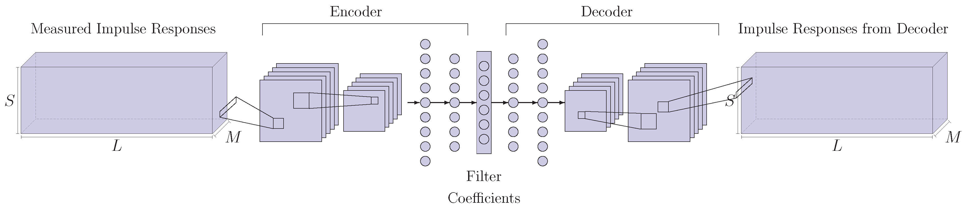
3.3. Autoencoder

An Autoencoder is a generative model [32] based on an encoder, a decoder and an internal representation that interconnects the two, often called latent space.

In our case, the encoder is composed of convolutional and fully connected layers, similar to the CNN of Section 3.2. The decoder performs the inverse mapping, thus, it is based on fully connected layers and de-convolutional layers. Filters coefficients are sampled from the internal representation, that has, thus, a size of $\mathcal{S}\times \mathcal{T}$. Impulse responses are used as input to the encoder, as shown in Figure 4.

The loss function for the autoencoder is defined as the sum of the Euclidean distance of Equation (3), and the reconstruction loss. The latter is expressed as the Euclidean distance between the input impulse response and the reconstructed one. Overall the loss for the autoencoder is:

$$\begin{array}{c}\hfill J_{AE}=\left(\alpha ·\sum _{m=1}^{\mathcal{M}}{∥|{\tilde{Y}}_m\left(\omega \right)|-|Y_{des}\left(\omega \right)|∥}_2+(1-\alpha )·\sum _{m=1}^{\mathcal{M}}\sum _{s=1}^{\mathcal{S}}{∥{\tilde{h}}_{m,s}\left(n\right)-h_{m,s}\left(n\right)∥}_2\right).\end{array}$$

(4)

The term $\alpha$ allows to weight the two losses, but for the rest of the paper it is kept equal to $0.5$.

4. Baseline Methods

To compare the proposed approach, we have selected two methods from the literature, namely the Fast Deconvolution (FD) from Kirkeby et al. [33] and the Steepest Descent inverse filter design (SD) [24]. These approaches are described and motivated in the following.

4.1. Frequency Deconvolution Method

The fast deconvolution method is described in Reference [33], where deconvolution is performed in the frequency domain and made fast by taking advantage of the Fast Fourier Transform (FFT) algorithm. A matrix of optimal filters is computed in the frequency domain according to the following

$$\mathbf{G}\left(k\right)={[{\mathbf{H}}^H\left(k\right)\mathbf{H}\left(k\right)+\beta \mathbf{I}]}^{-1}{\mathbf{H}}^H\left(k\right)\mathbf{A}\left(k\right),$$

(5)

where k is the FFT bin, $\mathbf{I}$ is the identity matrix, ${}^H$ is the Hermitian operator, $\mathbf{H}\left(k\right)$ contains the FFT of the impulse responses, $\mathbf{A}\left(k\right)$ contains the target frequency responses. The term $\beta$ is an empirical regularization term that is necessary to avoid extreme peaks in the inverse filters, that would result in an excessive length of the filters in the frequency domain. Once $\mathbf{G}\left(k\right)$ is computed, its inverse FFT is computed and a circular shift of $K/2$ samples is performed, where K is the FFT size. This method is used to design $\mathcal{S}$ different filters, one per loudspeaker, for a fair comparison with our approach.

The FD method is expressed as a least-squares optimization problem in the frequency domain. The loss is:

$$J={\mathbf{e}}^H\mathbf{e}+\beta {\mathbf{v}}^H\mathbf{v},$$

(6)

where $\mathbf{e}$ is the error and $\beta {\mathbf{v}}^H\mathbf{v}$ is a regularization term meant as an effort penalty proportional to the total energy of the filtered input signals to the sources $\mathbf{v}$. The problem is, thus expressed as a convex optimization problem, where the squared error is minimized by a unique solution that is analytically found in Reference [33] by imposing the gradient of the loss function to zero.

There are important differences between the proposed method and FD. In our framework there are no assumptions on the convexity of the error surface. The gradient of the loss J in the proposed method is a nonlinear function. Specifically, our loss can be expressed as a function f of the magnitude frequency response of the impulse responses $\mathbf{h}$ and of the network output $\mathbf{g}$. The network output, that is, the filter coefficients $\mathbf{g}$, in turn, is a nonlinear function of the network weights $\theta$ and the network input $\mathbf{u}$ (i.e., the impulse responses, when not specified differently). In more rigorous terms:

$$J=f\left(\right|\mathcal{F}\left(\mathbf{g}\right)|,|\mathcal{F}\left(\mathbf{h}\right)\left|\right).$$

(7)

$$\mathbf{g}=\varphi (\theta ,\mathbf{u}).$$

(8)

4.2. Steepest Descent Method

FIR filters can be obtained by applying the Steepest Descent algorithm to audio equalization [24,25].

The first step of the algorithm consists in defining a target impulse response:

$$d={[\underset{L+\mathcal{T}-1}{\underbrace{\begin{array}{ccccccc}0& \cdots & 0& 1& 0& \cdots & 0\end{array}}}]}^T,$$

(9)

where L is the length of the impulse response, ${}^T$ denotes the transpose operator, and $\mathcal{T}$ is the number of taps of the FIR filters. The filters are adapted to match the target impulse response:

$$y_m=h_{m,1}\ast g_1+h_{m,2}\ast g_2+\cdots +h_{m,\mathcal{S}}\ast g_{\mathcal{S}}=\sum _{s=1}^{\mathcal{S}}{h}_{m,s}\ast g_s\approx d,$$

(10)

where $g_s$ are the FIR filters, $h_{m,s}$ are the impulse responses and $y_m$ is the output at the m-th microphone.

The optimization goal is achieved by minimizing the cost function:

$$J=\left|\right|d_{\mathcal{M}}-y{\left|\right|}_2,$$

(11)

where y is the vector containing the output impulse response $y=[y_1,y_2,\dots ,y_{\mathcal{M}}]$ and $d_{\mathcal{M}}$ is the vector containing $\mathcal{M}$ times the target impulse response. The inverse system g can be obtained by:

$$g=H^{+}{d}_{\mathcal{M}},$$

(12)

where $H^{+}$ is the pseudo inverse of the system matrix $H=\left[\begin{array}{cccc}{H}_{1,1}& H_{1,2}& \cdots & H_{1,\mathcal{S}}\\ ⋮& ⋮& ⋮& ⋮\\ H_{\mathcal{M},1}& H_{\mathcal{M},2}& \cdots & H_{\mathcal{M},S}\end{array}\right]$ and its elements $H_{m,s}$ are $(L+\mathcal{T}-1)\times \mathcal{T}$ circular matrices composed by the impulse responses $h_{m,s}$ [24]:

$$H_{m,s}=\left[\begin{array}{cccc}{h}_{m,s}\left(0\right)& 0& \cdots & 0\\ h_{m,s}\left(1\right)& h_{m,s}\left(0\right)& \cdots & 0\\ ⋮& \ddots & \ddots & ⋮\\ h_{m,s}(L-1)& \cdots & ⋮& ⋮\\ 0& h_{m,s}(L-1)& \ddots & ⋮\\ 0& \cdots & 0& h_{m,s}(L-1).\end{array}\right]$$

(13)

If H is full rank, then $H^{+}=H^{-1}$.

The FIR filters are calculated adaptively: the gradient of the cost function $\nabla J$ is given by:

$$\nabla J=-2H^T{d}_{\mathcal{M}}+2H^{T}Hg$$

(14)

and the inverse system can be obtained by:

$$G(k+1)=G\left(k\right)-\mu \nabla J,$$

(15)

where $\mu$ is the step-size.

5. Experiments

The performance of the proposed and the baseline methods have been assessed by computer experiments using impulse responses measured inside real car cabins. Two car models have been considered, an Alfa Romeo Giulia and a Jeep Renegade. The Giulia was first taken for binaural equalization experiments ($\mathcal{M}=2$). The impulse responses were obtained using the sine sweep method [34] as implemented by the Aurora plugins (http://pcfarina.eng.unipr.it/Aurora_XP/index.htm). Sampling was done at 28.8 kHz with a Roland Octa-Capture audio interface, then the impulse responses were resampled to 48 kHz. A Kemar 45BA mannequin was placed on the driver’s seat; the distance between its ears is $d=18$ cm. The Giulia provides $\mathcal{S}=7$ loudspeakers—four door woofers, one subwoofer in the trunk, one speaker in the center of the dashboard and one speaker in the driver’s headrest, as shown in Figure 5a.

To assess the equalization performance of the proposed approach in a different environment we have measured the impulse responses of another car, a Jeep Renegade and measured the impulse responses at multiple listening points. Its cabin response has been measured using $\mathcal{M}=4$ omnidirectional microphone, one per seat. Three additional microphones have been mounted around microphone M2 for proximity tests, to assess the effect of head movements on the equalization performance. These microphones, labeled as PM1, PM2 and PM3 are placed at a distance of 6.5 cm (forward), 6.5 cm (backward) and 22.5 cm (lateral), respectively. For a one-ot-one comparison with the binaural tests done on the Giulia, a binaural mannequin was also mounted at the driver seat to capture binaural impulse responses. The sine sweep method has been used as well, in this case sampling at 48 kHz using an Audio Precision APX-586 analyzer and a Crown D-75A power amplifier to drive the loudspeakers. The Renegade loudspeakers are located in the car dashboard, on the four doors and a subwoofer is placed in the trunk.

The baseline methods have been implemented in Matlab (https://mathworks.com/products/matlab.html), while the proposed methods have been implemented in Python using Keras (https://keras.io/) with Tensorflow (https://www.tensorflow.org/) as backend. They have been executed on a machine with Intel Core i7-4930K 3.40 GHz clock processor, 32 GB of RAM and Nvidia GTX-Titan GPU with 12 GB of dedicated RAM.

The results are provided in terms of the mean square error (MSE) and average standard deviation $\overline{\sigma }$. The MSE of the magnitude response is calculated bin-by-bin for each microphone between the desired frequency response and the measured magnitude frequency response. The results are averaged between all microphones, that is,:

$$\overline{MSE}=\frac{1}{\mathcal{M}}\sum _{m=1}^{\mathcal{M}}\left(\frac{{\sum }_{\omega ={\omega }_l}^{{\omega }_h}{\left(|Y_m\left(\omega \right)|-|Y_{des}\left(\omega \right)|\right)}^2}{{\omega }_h-{\omega }_l}\right).$$

(16)

The average standard deviation $\overline{\sigma }$ is calculated as:

$$\overline{\sigma }=\frac{1}{\mathcal{M}}\sum _{m=1}^{\mathcal{M}}{\sigma }_m,$$

(17)

where ${\sigma }_m$ is the standard deviation of m-th microphone:

$${\sigma }_m=\sqrt{\frac{1}{{\omega }_h-{\omega }_l+1}{\displaystyle \sum _{\omega ={\omega }_l}^{{\omega }_h}}(10·lo{g}_{10}|F_m\left(\omega \right){|-D)}^2}$$

(18)

$$D=\frac{1}{{\omega }_h-{\omega }_l+1}\sum _{\omega ={\omega }_l}^{{\omega }_h}(10·lo{g}_{10}|F_m\left(\omega \right)\left|\right).$$

(19)

$F_m$ is the sum of the frequency responses on the m-th microphone without equalization filters or with equalization filters, following Reference [35].

Since the Giulia impulse responses have been originally sampled at 28.8 kHz, we set the upper frequency bound ${\omega }_h$ to 14.4 kHz. The lower frequency bound ${\omega }_l$ is set to 20 Hz to avoid unnecessary equalization below the human hearing range.

We desire the FIR filters to have linear phase, that is, be symmetric. Following the frequency deconvolution approach, we impose an odd number of taps for all methods.

Preliminary experiments were conducted to determine the values for the training hyperparameters. During these experiments we observed that a sufficiently high number of iterations allows the networks to converge to very low errors. The learning rate was set to $1·{10}^{-3}$ for all the proposed approaches. w was set to $100.0$ and the batch size is set to 1. The Adam optimizer [36] was used, with decay equal to $3·{10}^{-8}$ for all architectures. The number of iterations of the SD was set to 250,000, as in Reference [21]. A similar number of iterations, 200,000, was set for the proposed methods. This leaves enough time for convergence and allows direct comparison to the evolutionary algorithms in Reference [21], where the number of iterations times the agents gives approximately 200,000.

Four convolutional layers configurations were generated randomly. These were applied to the convolutional networks used in the CNN and AE architectures. The first convolutional layer has kernels of size $M\times 1$ while the second, if present, has kernels of size $1\times S$. The fully connected layers following the convolutional ones have been varied in their number (1, 2) and size. Four MLP architectures were derived from the convolutional ones by retaining the size of the fully connected layers. Three additional configurations have been added to achieve a number of trainable parameters similar to those of the CNN, as reported in

Table 1. The CNN and MLP configurations used in the experiments. The number of parameters are referred to filters of 1024-th order.

CNN				MLP
Configuration	Number of Kernels	Number of Units	Trainable Parameters	Configuration	Number of Units	Trainable Parameters
Conv #1	[48, 24]	[10]	7,481,943	MLP #1	[10]	6,798,935
Conv #2	[10, 5]	[100, 10]	3,826,153	MLP #2	[100, 10]	67,280,035
Conv #3	[100, 25]	[100, 100]	12,483,433	MLP #3	[100, 100]	67,934,875
Conv #4	[10]	[1000]	3,825,863	MLP #4	[1000]	679,183,175
				MLP #5	[100]	67,924,775
				MLP #6	[100, 100, 100]	67,944,975
				MLP #7	[5]	36,003,713
				MLP #8	[10, 1000, 1000]	14,914,185

.

6. Results

6.1. Alfa Romeo Giulia

Binaural equalization results are shown in

Table 2. Audio equalization results for the Alfa Romeo Giulia with binaural microphones. Please note that the $\overline{MSE}$ in the absence of equalization is 2.19, with $\overline{\sigma }$ 3.52. Best results for each column are highlighted in bold.

Filter Order	MLP			AE			CNN			FD ($\mathit{\beta }=0.1$)		SD
	Conf.	$\overline{MSE}$	$\overline{\mathit{\sigma }}$	Conf.	$\overline{MSE}$	$\overline{\mathit{\sigma }}$	Conf.	$\overline{MSE}$	$\overline{\mathit{\sigma }}$	$\overline{MSE}$	$\overline{\mathit{\sigma }}$	$\overline{MSE}$	$\overline{\mathit{\sigma }}$
512	MLP #5	0.32	2.877	Conv #1	9.72$·{10}^{-4}$	0.136	Conv #2	7.90$·{10}^{-4}$	0.122	0.18	2.52	0.40	1.95
640	MLP #8	0.36	2.730	Conv #1	3.80$·{10}^{-4}$	0.085	Conv #2	3.74$·{10}^{-4}$	0.084	0.15	2.34	0.35	1.72
768	MLP #5	0.46	2.796	Conv #1	1.66$·{10}^{-4}$	0.056	Conv #2	1.79$·{10}^{-4}$	0.058	0.14	2.23	0.33	1.60
896	MLP #2	0.45	2.799	Conv #1	1.07$·{10}^{-4}$	0.045	Conv #1	1.02$·{10}^{-4}$	0.044	0.12	2.07	0.31	1.54
1024	MLP #7	0.32	2.746	Conv #1	6.85$·{\mathbf{10}}^{-\mathbf{5}}$	0.036	Conv #1	6.31$·{\mathbf{10}}^{-\mathbf{5}}$	0.034	0.10	1.93	0.30	1.50

for the Alfa Romeo Giulia. The two proposed methods based on deep neural networks outperform significantly any other method in the test, while the MLP does not reach the same performance as the FD and the SD. The CNN achieves slightly better results compared to the convolutional AE despite being simpler in terms of implementation and computational cost. Best overall results have been achieved using the CNN with FIR filters of order 1024. Their magnitude frequency response is shown in Figure 6. Shorter filters designed by the convolutional methods are subject to a slight performance degradation, however, their MSE remains very low.

In Figure 7, we compare the non-equalized (green) and equalized (blue) magnitude frequency response at the dummy head left and right microphone obtained from the filters designed with the CNN and the baseline approaches. The CNN filters correct the frequency responses obtaining an exceptionally flat magnitude. No relevant peaks or notches are present in the equalized frequency response. The FD method achieves a rather flat spectrum, but peaks and notches are still visible. The SD presents the higher $\overline{MSE}$, while its $\overline{\sigma }$ is lower than the FD. Indeed, the frequency responses have less peaks, but the magnitude response is biased and sits below 0 dB. The same happens for other FIR filter orders.

The performance of the FD method is known to be dependent on the $\beta$ parameter, which can be adjusted as a fixed constant or a frequency-dependent parameter, usually having dominance in the denominator for very low and high frequencies, to avoid excessive gain in the inverse filter in those ranges or to avoid equalization at all. We have tested different configurations of $\beta$ to search for the best performance of the FD method for a given filter order.

Table 3. Effect of the parameter $\beta$ on the performance. The V-shaped configuration refers to a frequency-dependent $\beta$ with a minimum of ${10}^{-4}$ at 1 kHz and maxima of ${10}^{-1}$ at DC and Nyquist, varying linearly on a dB scale. The U-shaped configuration takes a value of ${10}^{-4}$ in the range 100 Hz–10 kHz and one elsewhere. Best results for each column are highlighted in bold.

$\mathit{\beta }$	$\overline{MSE}$	$\overline{\mathit{\sigma }}$
${10}^{-4}$	0.123	1.83
${10}^{-3}$	0.118	1.82
${10}^{-2}$	0.108	1.81
${10}^{-1}$	0.108	1.93
1	0.281	2.71
10	0.686	4.2
100	0.937	5.09
V-shaped	0.101	1.829
U-shaped	0.124	1.86

reports the MSE and sigma for several values of $\beta$ and for two frequency-dependent $\beta$ with filter order 1024. Although, theoretically, with lower $\beta$ the inversion should get closer to ideal, thus reaching a lower MSE, the filter order constraints the performance by truncating the very long ideal impulse response. A sweet spot is obtained for $\beta$ in the range ${10}^{-2}<\beta <{10}^{-1}$. With larger $\beta$ the performance decreases, as expected. Some frequency-dependent configurations for $\beta$ have been selected that obtain good results. The V-shaped one is able to reduce the MSE by a tiny amount, however, no significant improvement can be found by using a frequency-dependent $\beta$. Overall, the MSE values do not change much from those of Table 2, thus confirming that the choice of $\beta$ in the experiments above is not adversely affecting the performance.

As seen above, even though the elimination of the regularization term $\beta$ should lead to an almost perfect inversion, the ideal inverse response is limited by the filter order, thus increasing the MSE for very low $\beta$. On the contrary, the proposed approach seems to achieve a very low error even with short filters.

6.2. Jeep Renegade

Taking the CNN as the best of the proposed methods and the FD as the best among the baseline methods, we continue our experiments in a different cabin, increasing the complexity of the problem by increasing the number of microphones, that is, listening points, to equalize and by increasing their distance. We also conduct a binaural experimental case, as a one-to-one comparison to the Giulia case.

Table 4. Audio equalization results for the Jeep Renegade with binaural microphones and four microphones (one per seat). The FIR order is 1024.

Setup	CNN			FD $\mathit{\beta }=0.1$
	Conf	$\overline{MSE}$	$\overline{\mathit{\sigma }}$	$\overline{MSE}$	$\overline{\mathit{\sigma }}$
Binaural	#1	$6.19·{10}^{-5}$	0.035	0.05	1.21
4 seats	#1	$5.7·{10}^{-4}$	0.106	0.15	1.95

reports the results for filters of order 1024. As can be seen, the CNN achieves approximately the same results as in the Giulia on the binaural equalization scenario ($6.19·{10}^{-5}$ vs. $6.31·{10}^{-5}$). As expected, there is a performance decrease with the 4-seats equalization, however, the MSE is still extremely low ($5.7·{10}^{-4}$). With respect to the Giulia, the FD method achieves a reduction of the MSE in the binaural case. A slight degradation of the performance is found for the 4-seats equalization as well. In conclusion, despite the degradation of the performance, results are still far superior than the state of the art method even in the 4-point scenario.

6.3. Sensitivity to Head Movements

Small head movements may result in a degradation of the equalization performance. For this reason, we assessed the validity of the proposed approach in response to small and large head movements. We analyzed the frequency response at three additional points: PM1 and PM2 (small head movement) and PM3 (large head movement). Their frequency response is shown in Figure 8, while their $\overline{MSE}$ and $\overline{\sigma }$ are presented in

Table 5. Audio equalization results for microphone M2 and microphones PM1, PM2 and PM3. The evaluation is achieved by the experiments performed using the Jeep Renegade with four microphones (see Table 4).

Mic.	CNN		FD
	$\overline{MSE}$	$\overline{\mathbf{\sigma }}$	$\overline{MSE}$	$\overline{\mathbf{\sigma }}$
M2	$5.07·{10}^{-4}$	0.10	0.14	1.82
PM1	0.61	2.88	1.2	2.9
PM2	0.50	3.31	0.57	3.07
PM3	0.80	3.09	0.84	3.12

, and compared to the one at the M2 microphone, for reference. In line with theory, the error tends to rise for high frequencies, for which the wavelength is shorter or of the same order of magnitude as the distance between microphone M2, however, in the low end the response is almost flat.

This issue is common to many widely used offline equalization algorithms, including that in Reference [33]. These algorithms can be complemented with adaptive solutions to tune the filters in real-time. Several solutions have been previously proposed, based, for example, on Kalman filtering and Steepest Descent to adaptively track the frequency response [25] or on the virtual microphone technique [37]. The proposed method could also be expanded to equalize a broader area using multiple microphones concentrated around a volume of space surrounding the listener’s head.

6.4. Sensitivity to the Input

Finding the best input features and dimensions is an issue in audio tasks that usually has no clear answer, and requires, thus, experimentation. In this work, furthermore, we exploit deep neural networks as optimizing algorithms, which is rather uncommon in the signal processing literature. Up to our knowledge, there is no prior experience in the application of neural networks in such a configuration for the goal of generating audio filters, thus the choice of the input is not trivial. To improve our understanding of this task, we have performed a new batch of experiments to observe the role of the input features in the optimization task. Specifically, we want to assess the role of the input in driving the optimization process.

For these experiments the input matrix is filled with either: (a) random values changing at each iteration, (b) random values constant for all the training, (c) all ones, (d) all zeros. We kept the same matrix size used in previous experiments, in order to leave the input layers and the number of trainable parameters unchanged. We conducted these experiments with all the four CNN configurations and all four kinds of inputs, and generated FIR filters of order 1024 for the Alfa Romeo Giulia case. Results are shown in

Table 6. Effect of the input type on the results of the CNN (filter order 1024). For each case, the best result and the related configuration is reported.

Input	$\overline{MSE}$	$\overline{\mathit{\sigma }}$	Conf.
Impulse Responses	$6.31·{10}^{-5}$	0.034	Conv #1
Random Iteration	$0.14$	2.152	Conv #1
Random Fixed	$1.35·{10}^{-4}$	0.052	Conv #1
All 1s	$1.17·{10}^{-4}$	0.049	Conv #1
All 0s	ill-conditioned

. In case (a), results are comparable to the FD method, but worse than the ones achieved by the proposed method in Table 2. The fixed random input and a unitary matrix get much closer to the results seen in Table 2, but are still not on par with the best result of the test. Finally, with the null matrix, all filters coefficients are zero, making this method unsuitable to the optimization process. Overall, it seems that our method can gain some advantage from the use of the measured impulse responses as input features, however, the network is able to design suitable filters even with non-informative input content, gaining information about the problem setup from the loss, where the impulse responses are employed to calculate the distance.

6.5. Over-Determined Case

In the selected use cases, the number of filters is larger than the number of microphones. To assess the validity of the method in single-channel configurations and in the over-determined case ($\mathcal{M}>\mathcal{S}$) we have conducted further experiments selecting a subset of the available impulse responses, thus simulating the presence of a lower number of speakers. The results are reported in

Table 7. Audio equalization in the single-channel and over-determined cases. Setup is $\mathcal{M}\times \mathcal{S}$.

Car	Setup	CNN		FD
		$\overline{MSE}$	$\overline{\mathbf{\sigma }}$	$\overline{MSE}$	$\overline{\mathbf{\sigma }}$
Giulia	$1\times 1$	0.52	8.57	0.62	9.84
	$2\times 1$	0.57	7.81	0.64	9.19
Renegade	$1\times 1$	0.03	1.34	0.12	2.01
	$4\times 1$	0.22	2.76	0.44	3.62

. As can be seen, the CNN scores better than the FD, meaning that the optimal solution in the least-squares sense can be further improved by non-convex optimization techniques. The performance degradation from the $1\times 1$ case to the $2\times 1$ case is extremely low. This suggests that the two impulse responses are quite similar. On the other hand, the performance improvement achieved by the CNN with the $2\times 7$ or the $4\times 7$ cases (Table 2 and Table 4) with respect to the $1\times 1$ cases suggests that the proposed method is able to efficiently exploit a large number of filters to greatly reduce the error at all microphones.

6.6. Remarks

One concern related to the proposed filter design technique is the computational cost, since the design procedure requires a complete training of the network. However, despite the very large number of iterations set for the experiments, the loss decays exponentially as it is typical of neural networks. As an example, in the Alfa Romeo Giulia 1024-th order CNN experiments, the MSE decays below $1·{10}^{-4}$ after 4200 iterations. It is thus possible to set a desired error threshold and stop the training as soon as it is reached.

For what concerns the filters, we have concentrated our attention on the frequency response, without considering the phase. The Frequency Deconvolution method provides symmetrical, thus linear, phase frequency responses, while the Steepest Descent algorithm does not. We would expect an arbitrary phase response from the proposed approach, since we do not constrain the phase in any way. However, from all our experiments we observe an almost linear phase response, as seen in Figure 9, where this is compared with a linear phase response, showing a close match. As an example, the mean squared phase error compared against a perfectly linear phase response and averaged over all the filters generated in the 1024th-order CNN case from Table 2, is 0.8 rad.

Another important issue to consider is the group delay introduced by the filters. As shown by the results, the most performing ones in terms of frequency response equalization are 1024-th order. This filter length, however, may not be acceptable in some applications due to computational cost and the introduction of a group delay of 513 taps (approximately 1.1 ms at a 44,100 Hz sampling rate). Experimental tests have proven that FIR filters of 512-th order present very good equalization capabilities, inferior by 1 order of magnitude compared to the 1024-th order case, but still largely superior than baseline techniques.

6.7. Results Summary

To conclude this section, we report a brief summary of the experiments. We have performed binaural equalization experiments in two environments, the cabin of an Alfa Romeo Giulia and a Jeep Renegade. In Figure 10 we report the best results obtained for the best proposed architecture, a CNN and the best of the comparative methods, the FD method, a widely used approach for inversion of the impulse response in single and multipoint scenarios. As shown, the CNN architecture outperforms FD by several orders of magnitude (see Section 6.1), highlighted by the logarithmic-scaled plot, in both the mean squared error $\overline{MSE}$ and the standard deviation $\overline{\sigma }$. The best result achieved by the CNN in the binaural case has been obtained for the Jeep Renegade ($6.19·{10}^{-5}\overline{MSE}$ in Section 6.2).

With the Jeep Renegade, we also conducted tests with four equalization points, leaving all other parameters identical. The results are slightly lower, but still remarkable: $5.7·{10}^{-4}\overline{MSE}$, meaning that it is still feasible to obtain an almost flat equalization profile for four passengers at the same time. Furthermore, in Section 6.3 we have tested for performance degradation for head movements using three additional microphones around one of the reference microphones used for the 4-points equalization. The results show, in line with theory, a slight degradation of the performance at high frequency (see Figure 8), as with other multipoint equalization approaches.

Finally, we have analyzed the loss decay with the CNN and concluded that the number of training epochs can be reduced significantly, for example, from 200,000 to 4200 with a reasonable degradation of performance ($\overline{MSE}<{10}^{-4}$).

7. Conclusions

In this work, we have shown a binaural and a multipoint audio equalization system based on a deep neural network approach to tune FIR filter coefficients. We proposed the use of the back-propagation algorithm as an optimization method in order to train a neural network to produce FIR coefficients able to satisfy specific criteria provided as loss function.

Three neural network architectures—MLP, CNN, and AE—are compared with state-of-the-art methods. Results show that deep learning approaches outperform other techniques by several orders of magnitude, yielding extremely flat magnitude frequency responses with a quasi linear phase. Among the networks, the CNN provided best results. Additional experiments highlighted the ability of the CNN to converge to a solution that is slightly superior to the least-squares one even when the system to solve is over-determined, motivating further studies on non-convex optimization methods for audio equalization. Finally, the effect of head movements has been studied using additional microphones. The proposed technique cannot be used in a real-time context, thus other techniques can be envisioned to tune the filters adaptively by tracking the head movements, as suggested in Section 6.3. Another possibility is the extension of the current work to a broader area by using multiple microphones in the vicinity of the head.

Although the training stage can be heavy in computational cost, the convergence speed is quite fast, allowing a user to set a desired error threshold to stop the iterations as soon as the objective is reached.

Since the deep neural network approach has shown to be capable in the design of audio filters meeting the expected goals, this research topic may be expanded in the future to different applications and constraints.

Several topics have been left for future works and need to be addressed, such as a subjective evaluation and the design of IIR filters. Given their lower computational cost, compared to FIR filters, they may be suitable for real-time implementation. The use of psychoacoustically oriented metrics, such as 1/3 octave band smoothed frequency responses, may drive the optimization to a frequency response that better represents the human auditory perception. Finally, a thorough exploration of the hyperparameters, the input features and their size, may lead to smaller neural networks with the same performance, improving the filter design speed.