Low-Order Spherical Harmonic HRTF Restoration Using a Neural Network Approach


Abstract
1. Introduction
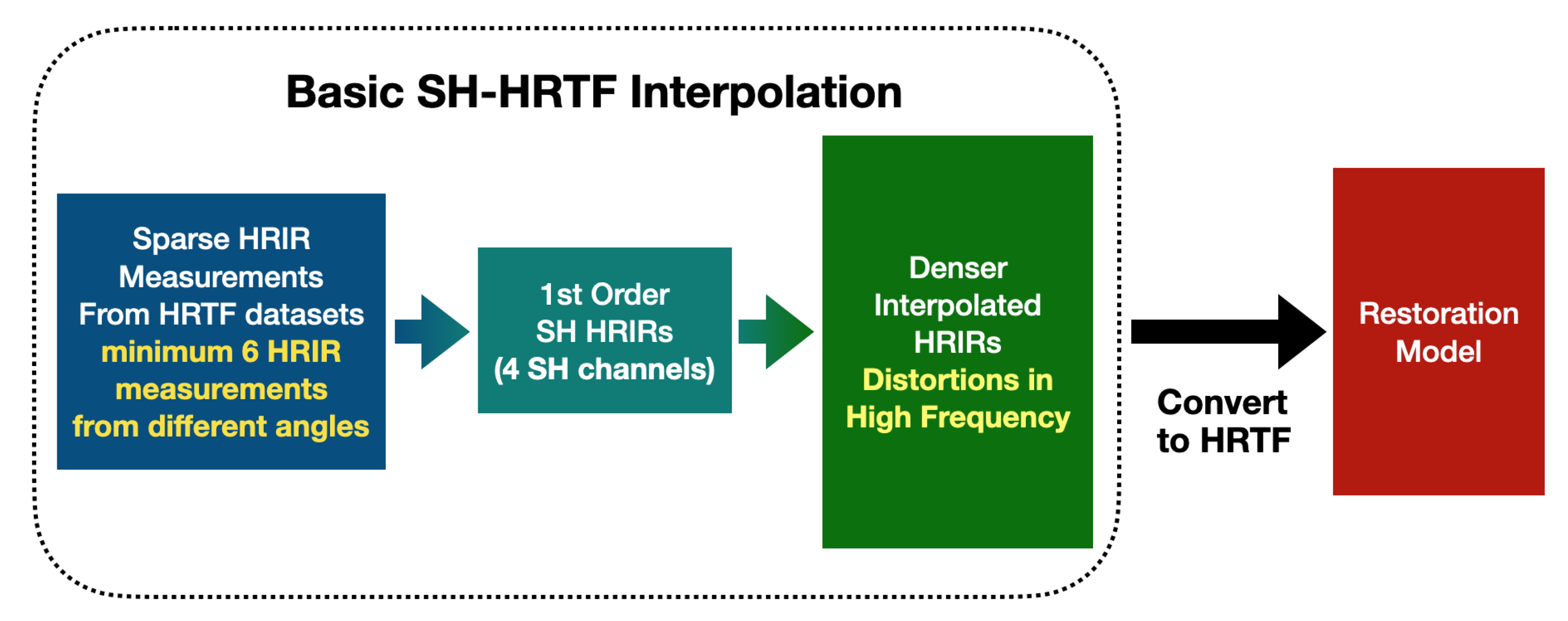
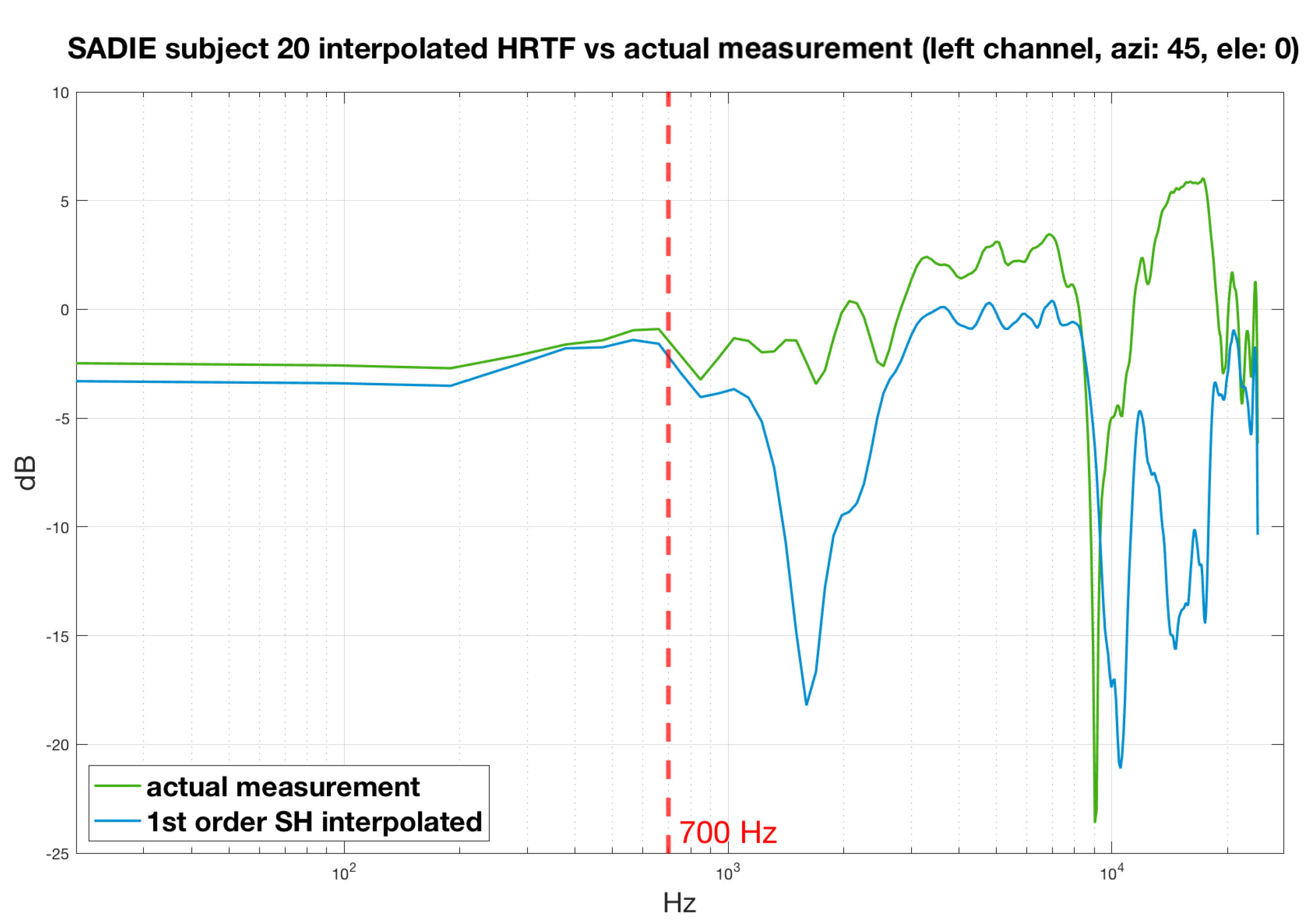
2. Spherical Harmonic HRTF Interpolation
3. Machine Learning HRTF Restoration
3.1. Data Pre-Processing
Data Selection
3.2. Baseline Model
3.3. Model Enhancement
3.3.1. Smaller Model
3.3.2. Model With Weight Decay
3.3.3. Model With Dropout
3.3.4. Combining Weight Decay and Dropout
3.3.5. Early Stopping
3.3.6. Training With More Data
3.3.7. Bigger Model
3.3.8. Summary
4. Evaluation
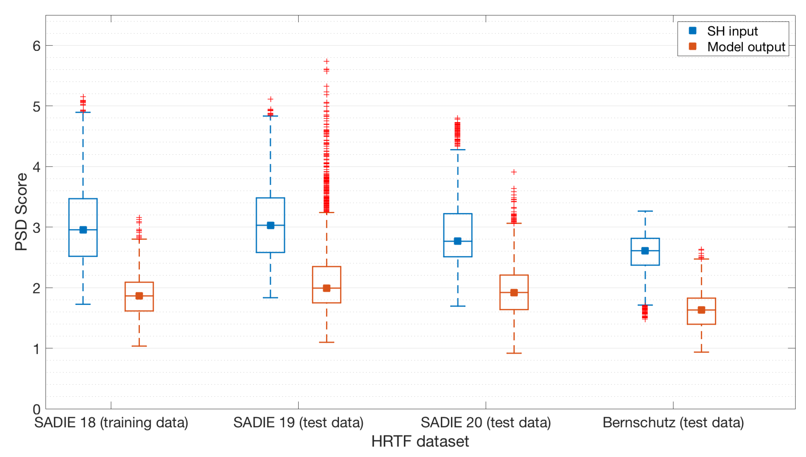
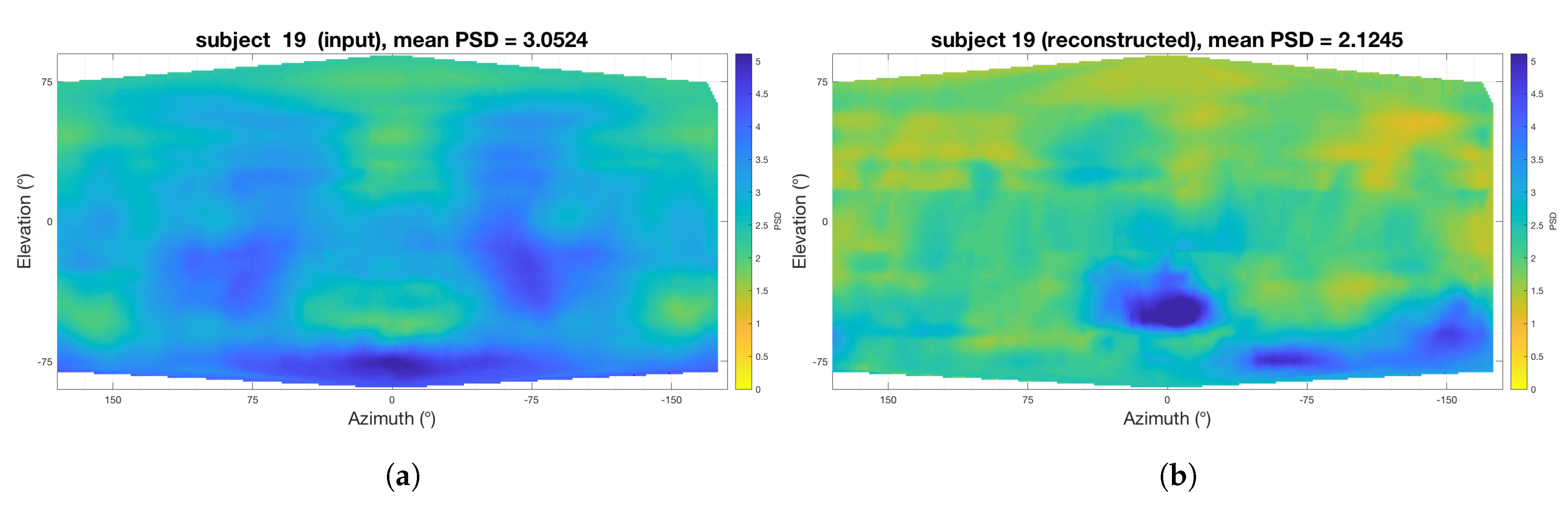
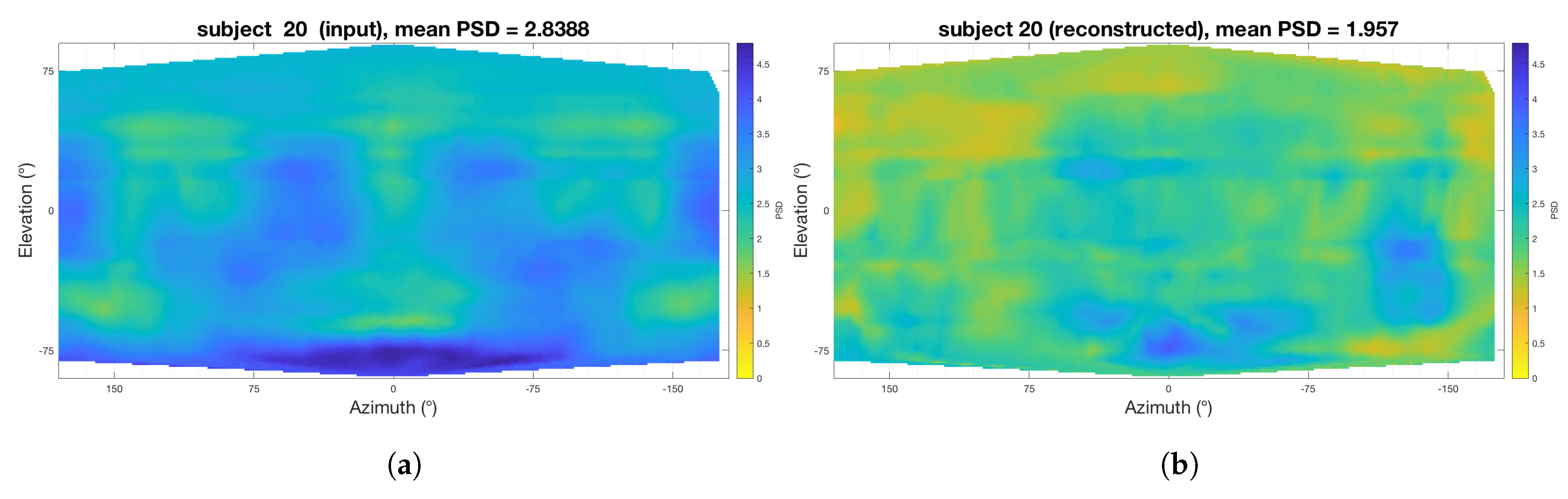
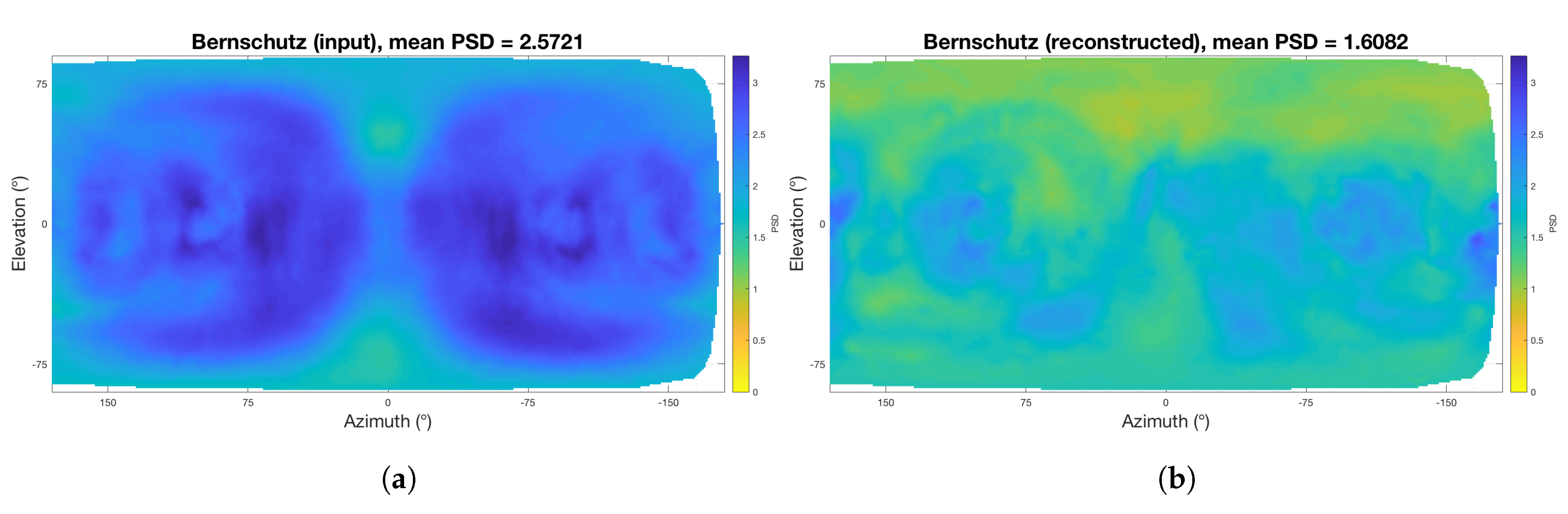
4.1. Perceptual Spectral Difference
4.2. Localisation Performance
5. Discussion and Future Work
6. Conclusions
Supplementary Materials
Author Contributions
Funding
Acknowledgments
Conflicts of Interest
Abbreviations
| AE | Auto-encoder |
| AMT | Auditory Modelling Toolbox |
| AR | Augmented Reality |
| CAE | Convolutional Auto-Encoder |
| DAE | Denoising Auto-Encoder |
| GANs | Generative Adversarial Networks |
| HRTF | Head Related Transfer Function |
| ILD | Interaural Level Difference |
| IQR | Interquartile Range |
| ITD | Interaural Time Difference |
| MAE | Mean Absolute Error |
| ML | Machine Learning |
| MSE | Mean Square Error |
| NN | Neural Networks |
| PSD | Perceptual Spectral Difference |
| RAM | Random Access Memory |
| ResNet | Residual Network |
| SH | Spherical Harmonic |
| SOFA | Spatially Oriented Format for Acoustics |
| TA | Time Alignment |
| VBAP | Vector Base Amplitude Panning |
| VR | Virtual Reality |
References
- Poirier-Quinot, D.; Katz, B.F. Impact of HRTF individualization on player performance in a VR shooter game I. In Proceedings of the AES International Conference on Spatial Reproduction, Tokyo, Japan, 7–9 August 2018; p. 7. [Google Scholar]
- Poirier-Quinot, D.; Katz, B.F. Impact of HRTF individualization on player performance in a VR shooter game II. In Proceedings of the AES International Conference on Audio for Virtual and Augmented Reality, Redmond, WA, USA, 20–22 August 2018; p. 8. [Google Scholar]
- Xie, B. Head-Related Transfer Function and Virtual Auditory Display, 2nd ed.; J. Ross Publishing: Plantation, FL, USA, 2013; p. 501. [Google Scholar]
- Howard, D.M.D.M.; Angus, J. Acoustics and Psychoacoustics, 4th ed.; Focal Press: Waltham, MA, USA, 2009. [Google Scholar] [CrossRef]
- Pulkki, V. Virtual sound source positioning using vector base amplitude panning. J. Audio Eng. Soc. 1997, 45, 456–466. [Google Scholar]
- Gerzon, M.A. Periphony: With-height sound reproduction. J. Audio Eng. Soc. 1973, 21, 2–10. [Google Scholar]
- Noisternig, M.; Musil, T.; Sontacchi, A.; Holdrich, R. 3D binaural sound reproduction using a virtual ambisonic approach. In Proceedings of the IEEE International Symposium on Virtual Environments, Human-Computer Interfaces and Measurement Systems, VECIMS’03, Lugano, Switzerland, 27–29 July 2003; pp. 174–178. [Google Scholar]
- Kearney, G.; Doyle, T. Height Perception in Ambisonic Based Binaural Decoding. In Proceedings of the Audio Engineering Society Convention 139, New York, NY, USA, 29 October–1 November 2015. [Google Scholar]
- Armstrong, C.; Chadwick, A.; Thresh, L.; Murphy, D.; Kearney, G. Simultaneous HRTF Measurement of Multiple Source Configurations Utilizing Semi-Permanent Structural Mounts. In Proceedings of the Audio Engineering Society Convention 143, New York, NY, USA, 18–21 October 2017. [Google Scholar]
- Armstrong, C.; Thresh, L.; Murphy, D.; Kearney, G. A perceptual evaluation of individual and non-individual HRTFs: A case study of the SADIE II database. Appl. Sci. 2018, 8, 2029. [Google Scholar] [CrossRef]
- Lee, G.W.; Kim, H.K. Personalized HRTF modeling based on deep neural network using anthropometric measurements and images of the ear. Appl. Sci. 2018, 8, 2180. [Google Scholar] [CrossRef]
- Katz, B.F. Boundary element method calculation of individual head-related transfer function. I. Rigid model calculation. J. Acoust. Soc. Am. 2001, 110, 2440–2448. [Google Scholar] [CrossRef]
- Young, K.; Kearney, G.; Tew, A.I. Loudspeaker Positions with Sufficient Natural Channel Separation for Binaural Reproduction. In Proceedings of the Audio Engineering Society International Conference on Spatial Reproduction—Aesthetics and Science, Tokyo, Japan, 7–9 August 2018. [Google Scholar]
- Young, K.; Tew, A.I.; Kearney, G. Boundary element method modelling of KEMAR for binaural rendering: Mesh production and validation. In Proceedings of the Interactive Audio Systems Symposium, York, UK, 23 September 2016; pp. 1–8. [Google Scholar]
- McKeag, A.; McGrath, D.S. Sound field format to binaural decoder with head tracking. In Proceedings of the Audio Engineering Society 6th Australian Reagional Convention, Melbourne, VIC, Australia, 10–12 September 1996; pp. 1–9. [Google Scholar]
- Noisternig, M.; Sontacchi, A.; Musil, T.; Holdrich, R. A 3D Ambisonic Based Binaural Sound Reproduction System. In Proceedings of the 24th AES International Conference on Multichannel Audio, The New Reality, Banff, AB, Canada, 26–28 June 2003. [Google Scholar]
- Zhu, J.Y.; Park, T.; Isola, P.; Efros, A.A. Unpaired Image-to-Image Translation Using Cycle-Consistent Adversarial Networks. In Proceedings of the IEEE International Conference on Computer Vision, Venice, Italy, 22–29 October 2017; pp. 2242–2251. [Google Scholar] [CrossRef]
- Isola, P.; Zhu, J.Y.; Zhou, T.; Efros, A.A. Image-to-image translation with conditional adversarial networks. In Proceedings of the 30th IEEE Conference on Computer Vision and Pattern Recognition (CVPR 2017), Honolulu, HI, USA, 21–26 July 2017; pp. 5967–5976. [Google Scholar] [CrossRef]
- Gamper, H. Head-related transfer function interpolation in azimuth, elevation, and distance. J. Acoust. Soc. Am. 2013, 134, EL547–EL553. [Google Scholar] [CrossRef]
- Grijalva, F.; Martini, L.C.; Florencio, D.; Goldenstein, S. Interpolation of Head-Related Transfer Functions Using Manifold Learning. IEEE Signal Process. Lett. 2017, 24, 221–225. [Google Scholar] [CrossRef]
- Hartung, K.; Braasch, J.; Sterbing, S.J. Comparison of different methods for the interpolation of head-related transfer functions. In Proceedings of the AES 16th International Conference: Spatial Sound Reproduction, Rovaniemi, Finland, 10–12 April 1999; pp. 319–329. [Google Scholar]
- Martin, R.L.; McAnally, K. Interpolation of Head-Related Transfer Functions; Air Operations Division Defence Science and Technology Organisation: Canberra, ACT, Australia, 2007.
- Evans, M.J.; Angus, J.A.S.; Tew, A.I. Analyzing head-related transfer function measurements using surface spherical harmonics. J. Acoust. Soc. Am. 1998, 104, 2400–2411. [Google Scholar] [CrossRef]
- Zotter, F.; Frank, M. Ambisonics, 1st ed.; Springer Topics in Signal Processing Series; Springer International Publishing: Cham, Switzerland, 2019; Volume 19. [Google Scholar] [CrossRef]
- Chapman, M.; Ritsch, W.; Musil, T.; Zmölnig, I.; Pomberger, H.; Zotter, F.; Sontacchi, A. A Standard for Interchange of Ambisonic Signal Sets Including a file standard with metadata. In Proceedings of the Ambisonics Symposium 2009, Graz, Austria, 25–27 June 2009; pp. 25–27. [Google Scholar]
- Daniel, J. Représentation de champs acoustiques, application à la transmission et à la reproduction de scènes sonores complexes dans un contexte multimédia. Ph.D. Thesis, University of Paris VI, Paris, France, 2000. [Google Scholar]
- Bertet, S.; Daniel, J.; Moreau, S. 3D Sound Field Recording with Higher Order Ambisonics—Objective Measurements and Validation of Spherical Microphone. In Proceedings of the 120th Audio Engineering Society Convention, Paris, France, 20–23 May 2006. [Google Scholar]
- Zaunschirm, M.; Schörkhuber, C.; Höldrich, R. Binaural rendering of Ambisonic signals by head-related impulse response time alignment and a diffuseness constraint. J. Acoust. Soc. Am. 2018, 143, 3616–3627. [Google Scholar] [CrossRef]
- Mckenzie, T.; Murphy, D.T.; Kearney, G. An Evaluation of Pre-Processing Techniques for Virtual Loudspeaker Binaural Ambisonic Rendering. In Proceedings of the EAA Spatial Audio Signal Processing symposium, Paris, France, 6–7 September 2019; pp. 149–154. [Google Scholar] [CrossRef]
- Sutton, R. The Bitter Lesson. 2019. Available online: http://www.incompleteideas.net/IncIdeas/BitterLesson.html (accessed on 29 October 2019).
- Yang, C.; Lu, X.; Lin, Z.; Shechtman, E.; Wang, O.; Li, H. High-resolution image inpainting using multi-scale neural patch synthesis. In Proceedings of the 30th IEEE Conference on Computer Vision and Pattern Recognition, CVPR 2017, Honolulu, HI, USA, 21–26 July 2017; pp. 4076–4084. [Google Scholar] [CrossRef]
- Nazeri, K.; Ng, E.; Joseph, T.; Qureshi, F.Z.; Ebrahimi, M. Edgeconnect: Generative image inpainting with adversarial edge learning. arXiv 2019, arXiv:1901.00212. [Google Scholar]
- Yan, Z.; Li, X.; Li, M.; Zuo, W.; Shan, S. Shift-net: Image inpainting via deep feature rearrangement. In Proceedings of the 15th European Conference on Computer Vision (ECCV), Munich, Germany, 8–14 September 2018; pp. 3–19. [Google Scholar] [CrossRef]
- Liu, G.; Reda, F.A.; Shih, K.J.; Wang, T.C.; Tao, A.; Catanzaro, B. Image Inpainting for Irregular Holes Using Partial Convolutions. In Proceedings of the 15th European Conference on Computer Vision (ECCV), Munich, Germany, 8–14 September 2018; pp. 89–105. [Google Scholar] [CrossRef]
- Antic, J. Jantic/DeOldify: A Deep Learning Based Project for Colorizing And Restoring Old Images (and Video!). 2019. Available online: https://github.com/jantic/DeOldify (accessed on 29 October 2019).
- Mao, X.; Shen, C.; Yang, Y.B. Image restoration using very deep convolutional encoder-decoder networks with symmetric skip connections. In Proceedings of the Advances in Neural Information Processing Systems 29 (NIPS 2016), Barcelona, Spain, 5–10 December 2016; pp. 2802–2810. [Google Scholar]
- Zhang, Y.; Tian, Y.; Kong, Y.; Zhong, B.; Fu, Y. Residual dense network for image restoration. IEEE Trans. Pattern Anal. Mach. Intell. 2020. [Google Scholar] [CrossRef] [PubMed]
- He, K.; Zhang, X.; Ren, S.; Sun, J. Deep residual learning for image recognition. In Proceedings of the IEEE Computer Society Conference on Computer Vision and Pattern Recognition, Las Vegas, NV, USA, 27–30 June 2016; pp. 770–778. [Google Scholar] [CrossRef]
- Goodfellow, I.; Pouget-Abadie, J.; Mirza, M.; Warde-Farley, D.; Ozair, S.; Courville, A.; Bengio, J. Generative adversarial nets. In Proceedings of the Advances in Neural Information Processing Systems 27 (NIPS 2014), Montreal, QC, Canada, 8–13 December 2014; pp. 1–9. [Google Scholar] [CrossRef]
- General Information on SOFA. 2013. Available online: https://www.sofaconventions.org/mediawiki/index.php/General_information_on_SOFA (accessed on 20 June 2019).
- SOFA—Spatially Oriented Format for Acoustics. 2015. Available online: https://github.com/sofacoustics/API_MO (accessed on 23 June 2019).
- Acoustics Research Institute. ARI HRTF Database. 2014. Available online: https://www.kfs.oeaw.ac.at/index.php?option=com_content&view=article&id=608&Itemid=606&lang=en#AnthropometricData (accessed on 11 July 2019).
- Bomhardt, R.; De La, M.; Klein, F.; Fels, J. A high-resolution head-related transfer function and three-dimensional ear model database A high-resolution head-related transfer function dataset and 3D ear model database. Proc. Meet. Acoust. J. Acoust. Soc. Am. 2016, 29. [Google Scholar] [CrossRef]
- Watanabe, K.; Iwaya, Y.; Suzuki, Y.; Takane, S.; Sato, S. Dataset of head-related transfer functions measured with a circular loudspeaker array. Acoust. Sci. Technol. 2014, 35, 159–165. [Google Scholar] [CrossRef]
- University of York. SADIE|Spatial Audio For Domestic Interactive Entertainment. 2014. Available online: https://www.york.ac.uk/sadie-project (accessed on 11 July 2019).
- Warusfel, O. Listen HRTF Database. 2003. Available online: http://recherche.ircam.fr/equipes/salles/listen/index.html (accessed on 11 July 2019).
- Bernschütz, B. A Spherical Far Field HRIR/HRTF Compilation of the Neumann KU 100. In Proceedings of the AIA–DAGA 2013 Conference on Acoustics, Merano, Italy, 18–21 March 2013; pp. 592–595. [Google Scholar]
- Sorber, L.; Barel, M.V.; Lathauwer, L.D. Unconstrained optimization of real functions in complex variables. SIAM J. Optim. 2012, 22, 879–898. [Google Scholar] [CrossRef]
- Kim, T.; Adalı, T. Approximation by Fully Complex Multilayer Perceptrons. Neural Comput. 2003, 15, 1641–1666. [Google Scholar] [CrossRef]
- Trabelsi, C.; Bilaniuk, O.; Zhang, Y.; Serdyuk, D.; Subramanian, S.; Santos, J.F.; Mehri, S.; Rostamzadeh, N.; Bengio, Y.; Pal, C. Deep Complex Networks. arXiv 2018, arXiv:1705.09792. [Google Scholar]
- Sarrof, A.M. Complex Neural Networks for Audio. Ph.D. Thesis, Dartmouth College, Hanover, NH, USA, 2018. [Google Scholar]
- Szegedy, C.; Liu, W.; Jia, Y.; Sermanet, P.; Reed, S.; Anguelov, D.; Erhan, D.; Vanhoucke, V.; Rabinovich, A. Going deeper with convolutions. In Proceedings of the IEEE Computer Society Conference on Computer Vision and Pattern Recognition, Boston, MA, USA, 7–12 June 2015; pp. 1–9. [Google Scholar] [CrossRef]
- Goodfellow, I.; Bengio, Y.; Courville, A. Deep Learning. Nature 2016, 521, 800. [Google Scholar] [CrossRef]
- Geirhos, R.; Rubisch, P.; Michaelis, C.; Bethge, M.; Wichmann, F.A.; Brendel, W. ImageNet-trained CNNs are biased towards texture; increasing shape bias improves accuracy and robustness. arXiv 2018, arXiv:1811.12231. [Google Scholar]
- Paszke, A.; Gross, S.; Chintala, S.; Chanan, G.; Yang, E.; DeVito, Z.; Lin, Z.; Desmaison, A.; Antiga, L.; Lerer, A. Automatic differentiation in PyTorch. In Proceedings of the NIPS 2017 Workshop Autodiff, Long Beach, CA, USA, 9 December 2017. [Google Scholar]
- Paszke, A.; Gross, S.; Massa, F.; Lerer, A.; Bradbury, J.; Chanan, G.; Killeen, T.; Lin, Z.; Gimelshein, N.; Antiga, L.; et al. PyTorch: An Imperative Style, High-Performance Deep Learning Library. In Advances in Neural Information Processing Systems 32; Wallach, H., Larochelle, H., Beygelzimer, A., d’Alché-Buc, F., Fox, E., Garnett, R., Eds.; Curran Associates, Inc.: Red Hook, NY, USA, 2019; pp. 8024–8035. [Google Scholar]
- Masters, D.; Luschi, C. Revisiting small batch training for deep neural networks. arXiv 2018, arXiv:1804.07612. [Google Scholar]
- Wilson, D.R.; Martinez, T.R. The general inefficiency of batch training for gradient descent learning. Neural Netw. 2003, 16, 1429–1451. [Google Scholar] [CrossRef]
- Kingma, D.P.; Ba, J. Adam: A Method for Stochastic Optimization. arXiv 2015, arXiv:1412.6980. [Google Scholar]
- Krogh, A.; Hertz, J.A. A Simple Weight Decay Can Improve Generalization. In Advances in Neural Information Processing Systems 4; Moody, J.E., Hanson, S.J., Lippmann, R.P., Eds.; Morgan-Kaufmann: Burlington, MA, USA, 1992; pp. 950–957. [Google Scholar]
- Smith, L.N. A disciplined approach to neural network hyper-parameters: Part 1—Learning rate, batch size, momentum, and weight decay. arXiv 2018, arXiv:1803.09820. [Google Scholar]
- Loshchilov, I.; Hutter, F. Decoupled Weight Decay Regularization. arXiv 2017, arXiv:1711.05101. [Google Scholar]
- Hinton, G.E.; Krizhevsky, A.; Sutskever, I. System and Method for Addressing Overfitting in a Neural Network. U.S. Patent US14/015,768, 8 February 2016. [Google Scholar]
- Srivastava, N.; Hinton, G.; Krizhevsky, A.; Sutskever, I.; Salakhutdinov, R. Dropout: A Simple Way to Prevent Neural Networks from Overfitting. J. Mach. Learn. Res. 2014, 15, 1929–1958. [Google Scholar]
- Baldi, P.; Sadowski, P. Understanding dropout. Adv. Neural Inf. Process. Syst. 2013, 1–9. [Google Scholar] [CrossRef]
- Coursera. Other Regularization Methods—Practical Aspects of Deep Learning. Available online: https://www.coursera.org/lecture/deep-neural-network/other-regularization-methods-Pa53F (accessed on 1 January 2020).
- Armstrong, C.; McKenzie, T.; Murphy, D.; Kearney, G. A perceptual spectral difference model for binaural signals. In Proceedings of the 145th Audio Engineering Society International Convention, AES 2018, New York, NY, USA, 17–19 October 2018; pp. 1–5. [Google Scholar]
- Baumgartner, R.; Majdak, P.; Laback, B. Modeling sound-source localization in sagittal planes for human listeners. J. Acoust. Soc. Am. 2014, 136, 791–802. [Google Scholar] [CrossRef] [PubMed]
- May, T.; Van De Par, S.; Kohlrausch, A. A probabilistic model for robust localization based on a binaural auditory front-end. IEEE Trans. Audio Speech Lang. Process. 2011, 19, 1–13. [Google Scholar] [CrossRef]
- Søndergaard, P.; Majdak, P. The Auditory Modeling Toolbox. In The Technology of Binaural Listening; Blauert, J., Ed.; Springer: Berlin/Heidelberg, Germany, 2013; pp. 33–56. [Google Scholar]
- Aggarwal, C.C. Neural Networks and Deep Learning: A Textbook; Springer International Publishing: Cham, Switzerland, 2018. [Google Scholar]
- Zur, R.M.; Jiang, Y.; Pesce, L.L.; Drukker, K. Noise injection for training artificial neural networks: A comparison with weight decay and early stopping. Med. Phys. 2009, 36, 4810–4818. [Google Scholar] [CrossRef]
- He, Z.; Rakin, A.S.; Fan, D. Parametric noise injection: Trainable randomness to improve deep neural network robustness against adversarial attack. In Proceedings of the IEEE Conference on Computer Vision and Pattern Recognition, Long Beach, CA, USA, 16–20 June 2019; pp. 588–597. [Google Scholar]
- Gatys, L.; Ecker, A.; Bethge, M. A Neural Algorithm of Artistic Style. J. Vis. 2016, 16, 326. [Google Scholar] [CrossRef]
- Zhang, M.; Zheng, Y. Hair-GANs: Recovering 3D Hair Structure from a Single Image. arXiv 2018, arXiv:1811.06229. [Google Scholar]
- Brock, A.; Donahue, J.; Simonyan, K. Large Scale GAN Training for High Fidelity Natural Image Synthesis. Vet. Immunol. Immunopathol. 2018, 166, 33–42. [Google Scholar] [CrossRef]
- Salimans, T.; Goodfellow, I.; Zaremba, W.; Cheung, V.; Radford, A.; Chen, X. Improved techniques for training GANs. In Proceedings of the Neural Information Processing Systems 2016, Barcelona, Spain, 5–10 December 2016; pp. 2234–2242. [Google Scholar]


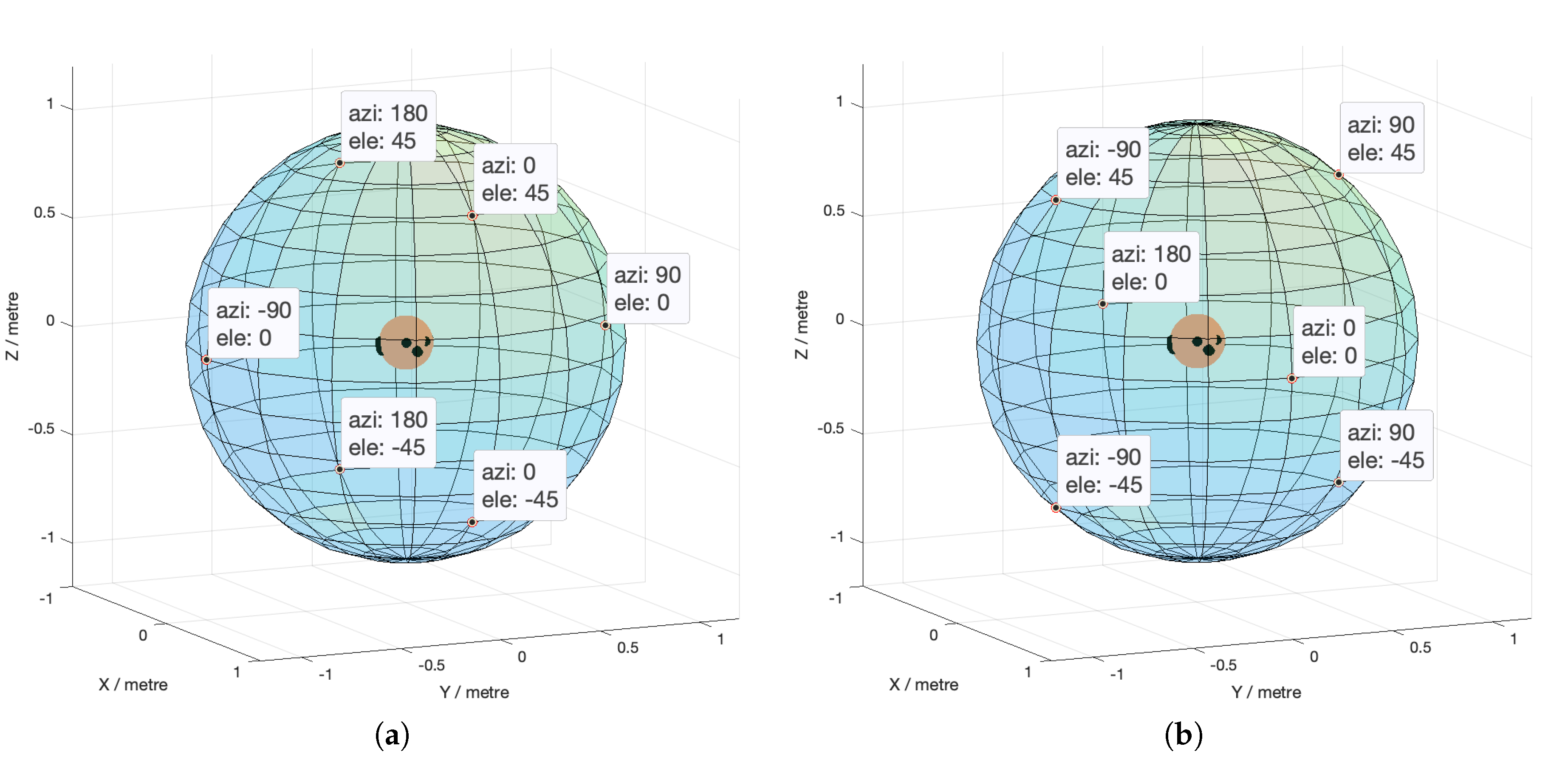
| Azimuth | Elevation | |
|---|---|---|
| 1 | 90.0 | 0.0 |
| 2 | 270.0 (or −90.0) | 0.0 |
| 3 | 0.0 | 45.0 |
| 4 | 0.0 | −45.0 |
| 5 | 180.0 | 45.0 |
| 6 | 180.0 | −45.0 |
| Azimuth | Elevation | |
|---|---|---|
| 1 | 0.0 | 0.0 |
| 2 | 180.0 | 0.0 |
| 3 | 90.0 | 45.0 |
| 4 | 90.0 | −45.0 |
| 5 | 270.0 (or −90.0) | 45.0 |
| 6 | 270.0 (or −90.0) | −45.0 |
| HRTF Dataset | Training and Validation | Testing |
|---|---|---|
| SADIE I | ✔ | |
| SADIE II (besides subject 19 and 20) | ✔ | |
| IRCAM Listen | ✔ | |
| ARI | modified | |
| ITA | modified | |
| RIEC | modified | |
| SADIE II (subject 19 and 20) | ✔ | |
| Bernschutz KU100 | ✔ |
| Comparison of Results Between Mono and Stereo Inputs (Lower Is Better) | ||||||
|---|---|---|---|---|---|---|
| Model | Overall Mean | Training | Validation | SADIE 20 | Bernschutz | Test Mean |
| Baseline (mono) | 50.66 | 31.40 | 33.94 | 62.27 | 75.04 | 68.65 |
| Baseline (stereo) | 44.46 | 28.17 | 30.17 | 52.34 | 67.17 | 59.75 |
| MSE With Different Loss Functions (Lower the Better) | ||||||
|---|---|---|---|---|---|---|
| Model | Overall Mean | Training | Validation | SADIE 20 | Bernschutz | Test Mean |
| Baseline (MSE loss) | 44.97 | 27.38 | 29.43 | 58.14 | 64.92 | 61.53 |
| Baseline (L1 loss) | 44.04 | 28.16 | 30.14 | 53.66 | 64.18 | 58.92 |
| Baseline (Smooth L1 loss) | 44.46 | 28.17 | 30.17 | 52.34 | 67.17 | 59.75 |
| Comparison of Results with and without Data from ARI, ITA and RIEC (Lower is Better). | ||||||
|---|---|---|---|---|---|---|
| Model | Overall Mean | Training | Validation | SADIE 20 | Bernschutz | Test Mean |
| Baseline (without extra data) | 45.28 | 18.29 | 20.55 | 51.33 | 90.93 | 71.13 |
| Baseline (with extra data) | 44.46 | 28.17 | 30.17 | 52.34 | 67.17 | 59.75 |
| Compare the Results From Different Models (Lower the Better) | ||||||
|---|---|---|---|---|---|---|
| Model | Overall Mean | Training | Validation | SADIE 20 | Bernschutz | Test Mean |
| A. Baseline | 44.46 | 28.17 | 30.17 | 52.34 | 67.17 | 59.76 |
| B. Smaller model | 45.51 | 19.54 | 21.52 | 51.62 | 89.35 | 70.48 |
| C. With weight decay | 46.04 | 28.59 | 30.96 | 52.75 | 71.89 | 62.32 |
| D. With dropout | 46.47 | 29.14 | 30.08 | 54.52 | 72.15 | 63.33 |
| E. With weight decay and dropout (proposed model) | 45.48 | 29.85 | 30.61 | 47.21 | 74.23 | 60.72 |
| F. With weight decay and dropout (early stopped at 111 epoch) | 49.78 | 40.92 | 41.00 | 47.18 | 70.04 | 58.61 |
| G. Baseline trained withextra data | 39.36 | 19.74 | 20.09 | 59.87 | 57.72 | 58.80 |
| H. With weight decay and dropout and trained with extra data | 41.44 | 22.49 | 22.07 | 59.69 | 61.50 | 60.60 |
| I. Bigger model without weight decay and trained with extra data | 31.38 | 7.83 | 10.61 | 56.88 | 50.22 | 53.55 |
| SADIE 18 (Training Data) | SADIE 19 (Hold Out) | SADIE 20 (Hold Out) | Bernschutz KU 100 | |
|---|---|---|---|---|
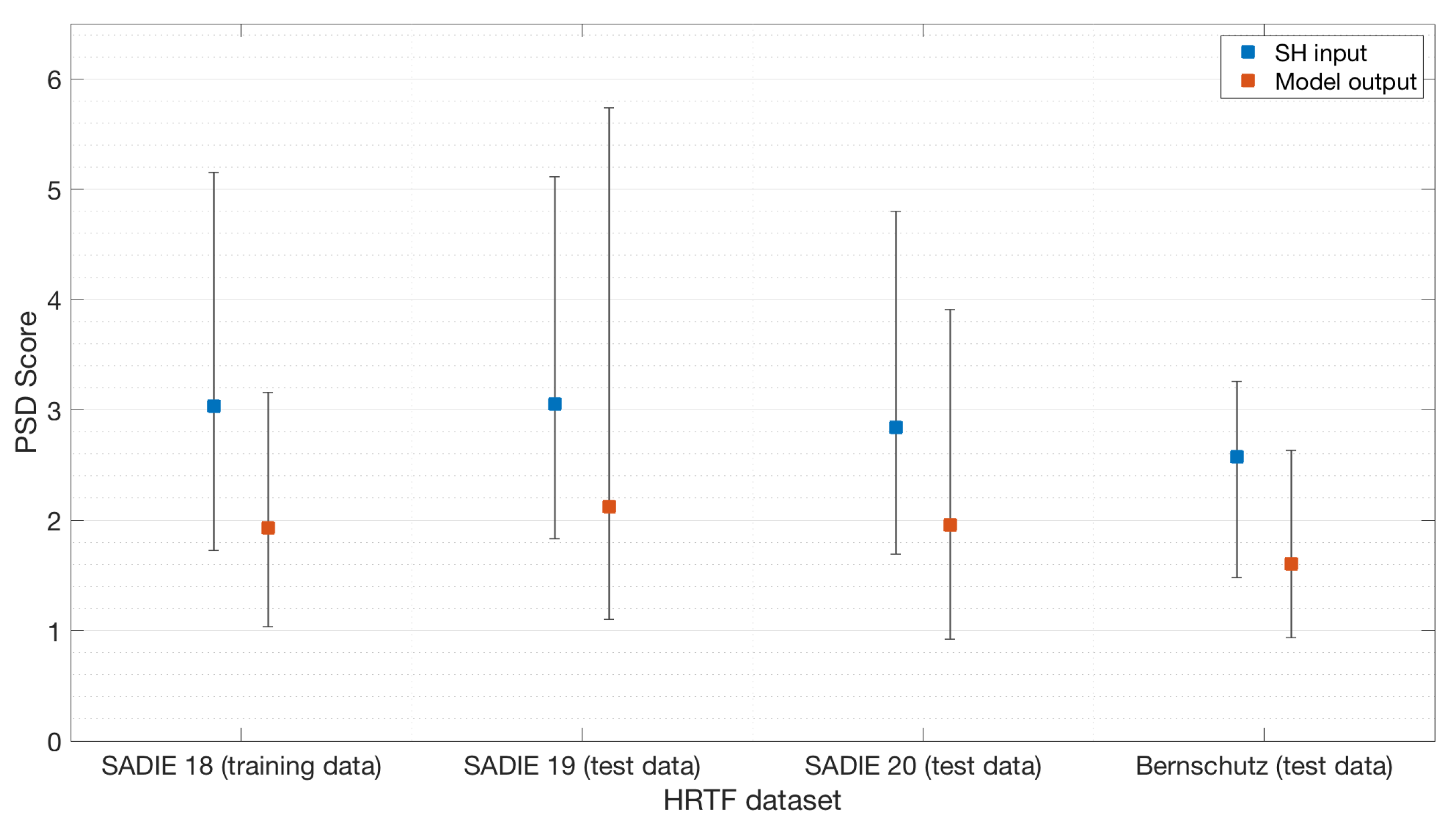
| PSD (sones) (SH input) | 3.03 | 3.05 | 2.84 | 2.57 |
| PSD (sones) (model output) | 1.93 | 2.12 | 1.96 | 1.61 |
| Frontal azimuth mean error (SH input) | 20.81 | 25.36 | 30.00 | 39.67 |
| Frontal azimuth mean error (model output) | 19.29 | 17.47 | 15.84 | 18.98 |
| Sagittal RMS error (deg) (SH input) | 40.7 | 38.6 | 37.5 | 38.1 |
| Sagittal RMS error (deg) (model output) | 44.3 | 43.7 | 39.3 | 41.4 |
| Sagittal quadrant errors (%) (SH input) | 11.5 | 9.1 | 7.6 | 7.1 |
| Sagittal quadrant errors (%) (model output) | 24.8 | 25.2 | 14.7 | 12.4 |
© 2020 by the authors. Licensee MDPI, Basel, Switzerland. This article is an open access article distributed under the terms and conditions of the Creative Commons Attribution (CC BY) license (http://creativecommons.org/licenses/by/4.0/).
Share and Cite
Tsui, B.; Smith, W.A.P.; Kearney, G. Low-Order Spherical Harmonic HRTF Restoration Using a Neural Network Approach. Appl. Sci. 2020, 10, 5764. https://doi.org/10.3390/app10175764
Tsui B, Smith WAP, Kearney G. Low-Order Spherical Harmonic HRTF Restoration Using a Neural Network Approach. Applied Sciences. 2020; 10(17):5764. https://doi.org/10.3390/app10175764
Chicago/Turabian StyleTsui, Benjamin, William A. P. Smith, and Gavin Kearney. 2020. "Low-Order Spherical Harmonic HRTF Restoration Using a Neural Network Approach" Applied Sciences 10, no. 17: 5764. https://doi.org/10.3390/app10175764
APA StyleTsui, B., Smith, W. A. P., & Kearney, G. (2020). Low-Order Spherical Harmonic HRTF Restoration Using a Neural Network Approach. Applied Sciences, 10(17), 5764. https://doi.org/10.3390/app10175764