Motion Planning for Autonomous Vehicles Considering Longitudinal and Lateral Dynamics Coupling

Abstract

Vehicles are highly coupled and multi-degree nonlinear systems. The establishment of an appropriate vehicle dynamical model is the basis of motion planning for autonomous vehicles. With the development of autonomous vehicles from L2 to L3 and beyond, the automatic driving system is required to make decisions and plans in a wide range of speeds and on bends with large curvature. In order to make precise and high-quality control maneuvers, it is important to account for the effects of dynamical coupling in these working conditions. In this paper, a new single-coupled dynamical model (SDM) is proposed to deal with the various dynamical coupling effects by identifying and simplifying the complicated one. An autonomous vehicle motion planning problem is then formulated using the nonlinear model predictive control theory (NMPC) with the SDM constraint (NMPC-SDM). We validated the NMPC-SDM with hardware-in-the-loop (HIL) experiments to evaluate improvements to control performance by comparing with the planners original design, using the kinematic and single-track models. The comparative results show the superiority of the proposed motion planning algorithm in improving the maneuverability and tracking performance.

1. Introduction

The popularization of autonomous vehicles is of great significance in improving road safety, traffic efficiency, and so on [1,2]. With the increasing levels of automation, motion planning, as a key subsystem of automatic driving systems, faces more challenges, such as nonlinear and coupling vehicle dynamics, spatial and temporal non-convex constraints, unknown and varying disturbances from the environment, and so on [3]. According to the basic theory and implementation principle, there are three main types of approach for the design of a motion planning algorithm, which are the artificial potential field (APF), the sampling-based method, and the optimal control method [4,5,6,7].

The APF constructs the potential field of vehicle motion according to the target attraction and the obstacle repulsion, and then searches for the shortest path to the target based on the gradient of the potential field [8,9,10]. An advantage is that the computation cost is low. However, the algorithm only generates the field for current vehicle state and environment information, thus, it can hardly account for future driving performances.

The basic idea of the sampling-based method is to convert the continuous planning problem into a discrete-and-search one. It first discretizes the configuration space into a series of sample points, then searches for a sequence of points that meet the task requirements [11,12]. The rapidly-exploring random tree is one of the most commonly used ones [13,14,15]. It has the advantages of better real-time performance and better search in the spatiotemporal domain. However, the inherent random mechanism makes it impossible to effectively deal with the constraints of vehicle dynamics.

Limited by their theoretical fundamentals, neither of the methods above can consider the nonlinear dynamics and safety constraints of obstacles [16]. This causes the planning module to generate control commands that may exceed the vehicle’s executable ability. Accordingly, the actual state trajectory will deviate from the desired one [17]. To solve the problems mentioned above, optimal control based schemes have been investigated widely in recent years. Among them, model predictive control (MPC) has received more attention because it puts the finite horizon optimal motion planning in continuous state space and can handle nonlinear dynamics, as well as environmental disturbances.

Essentially, MPC is a model-based approach, and its performance is greatly affected by the accuracy and complexity of the model. Gao et al. designed a nonlinear MPC (NMPC)-based planner for obstacle avoidance by considering the vehicle as a point-mass [18]. This model treats the vehicle as a particle, regardless of vehicle geometry and tire dynamics. This will produce a large predictive error in dynamical conditions and also increase the requirements of the path tracking module [19]. The point-mass model is replaced by a nonlinear kinematic model in [20] and an extended kinematic model over a three dimensional motion surface is presented in [21] for off-road navigation and control. But both point-mass and kinematic models only can describe vehicle behavior at low speed. At high speed, the cornering characteristics of tires are not negligible [22]. A data-driven statistical vehicle model is proposed in [23], which simultaneously describes the control constraints, actuator delay and vehicle dynamics. However, this model contains both continuous and discrete states. Carvalho et al. proposed a one-level NMPC planner for high-speed obstacle avoidance using a four-wheel nonlinear dynamical model with the Fiala tire constraints [24]. However, such complex models greatly increase the consumption of computational resource. To increase the real-time performance, Yadollah et al. reduced the high degree model to the single-track model and presented a field-based model predictive path-planning controller for high-speed conditions [25]. This single-track model is simplified with the small angle assumption and ignores the coupling effects between lateral and longitudinal dynamics. In essence, such coupling is not negligible when the steering angle becomes large enough, which easily happens at low speed.

The point-mass model and kinematic model are simplified to facilitate the motion planning and they are not applicable to dynamical driving conditions, for example, driving on a curve at speed. Although the complex nonlinear dynamic model is accurate enough, it is too complicated to be used for the design of a motion planner. The simplified single-track model doesn’t consider the coupling among longitudinal and lateral dynamics and is only applicable to the condition that the steering angle is small.

The main contributions of this paper can be summarized as follows:

(1)

Based on the statistical results of naturalistic driving data, a nonlinear vehicle model describing both longitudinal and lateral dynamics in the normal operating range was first established. It was simplified to a single-coupled dynamical model (SDM) with enough accuracy by analyzing the transfer characteristics and dynamical coupling effects at the equilibrium points numerically. This simplified model has a good balance between model accuracy and complexity.

(2)

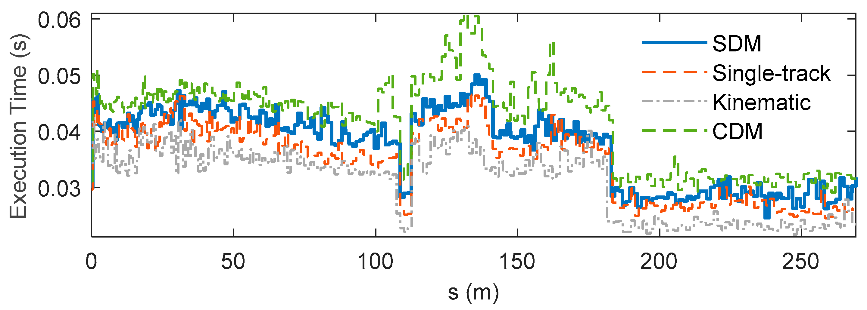
By using SDM, a NMPC-based motion planner was further designed considering the coupling effects of lateral and longitudinal dynamics. The improvement of control performance was validated by several comparative hardware-in-the-loop (HIL) experiments under different dynamical driving conditions.

Motion planning at the handling limits is also an important research topic. A multi-layered graph-based trajectory planner was designed for autonomous racing in [26,27], which can achieve a maximum speed of 212 km/h. A comprehensive survey of this topic is beyond the scope of our discussion, since our work focuses on motion planning under normal driving conditions for urban and highway autonomous driving. Interested readers are referred to [26,27] for more details. The rest of the paper is organized as follows. Section 2 introduces a statistical analysis of the operating range; Section 3 establishes the coupling dynamical model and simplifies it to SDM by numerical analysis; Section 4 constructs the NMPC motion planning problem and describes the HIL experiments conducted under different scenarios; and finally Section 5 concludes the paper.

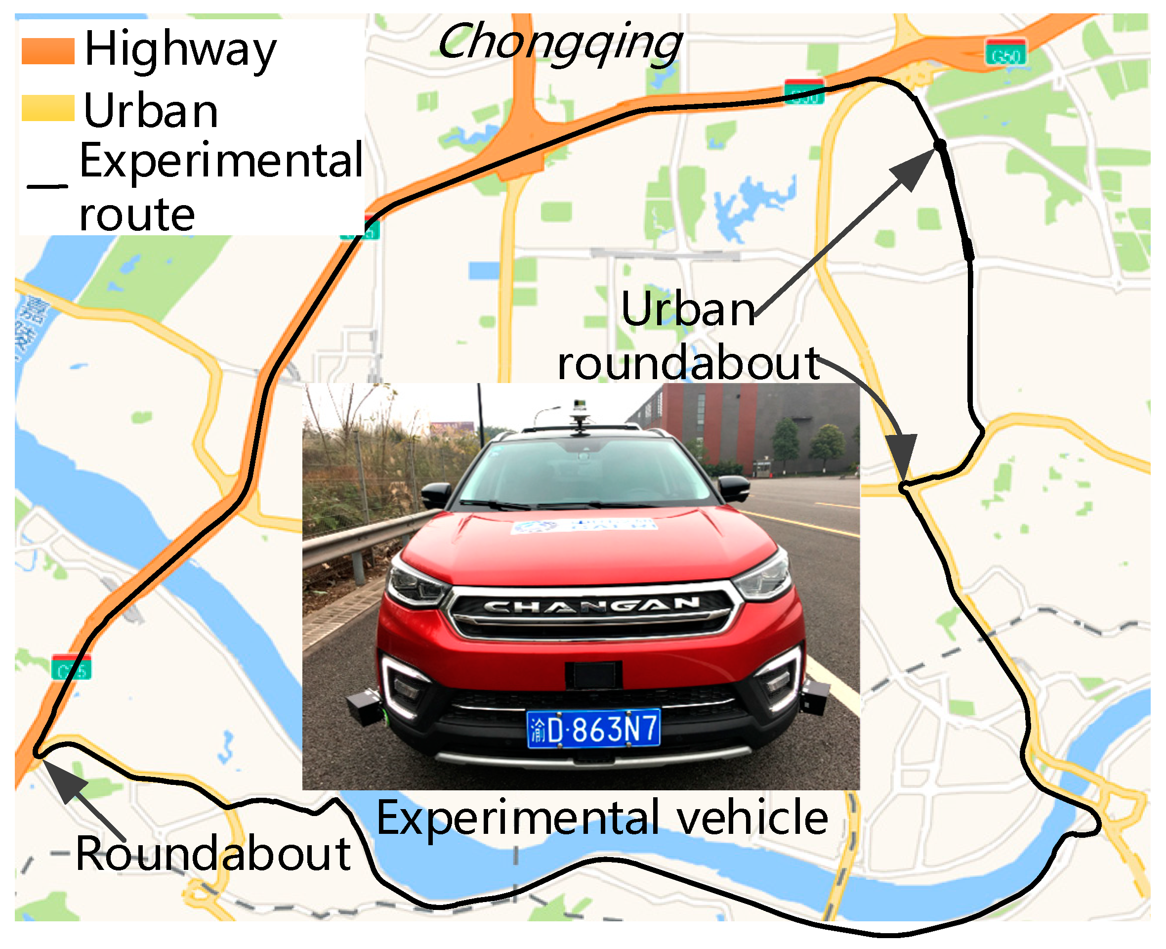
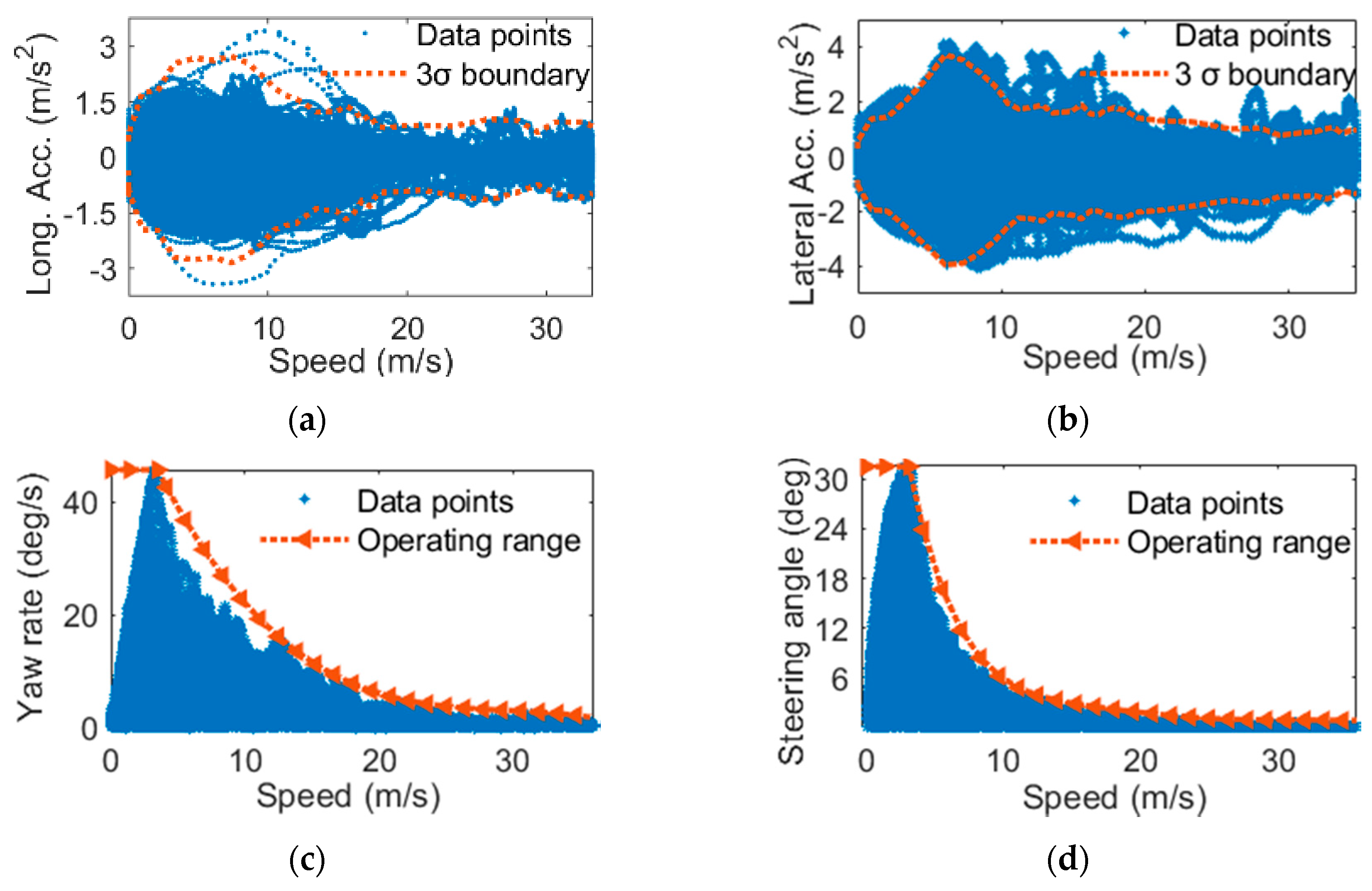
2. Statistical Analysis of Operating Range

When modelling vehicle dynamics for motion planning, the following are three typical issues [28,29]:

(1)

Using linear or nonlinear tire models;

(2)

Whether the transfer of the vertical load is negligible;

(3)

Whether the coupling between the longitudinal and lateral dynamics can be considered.

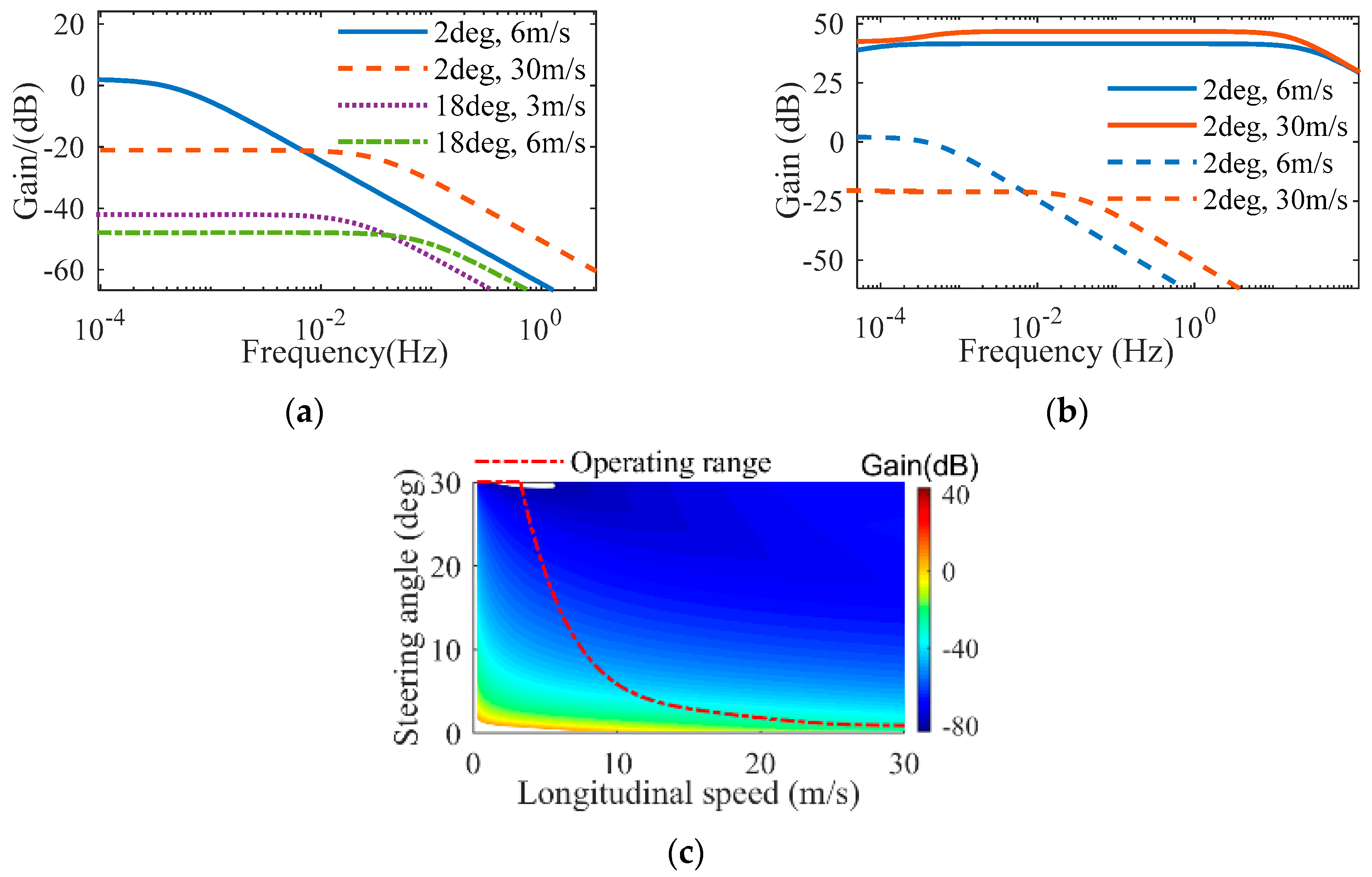
Methods of dealing with these problems are directly related to the operation conditions. Therefore, the naturalistic field operational test (FOT) was adopted to study the working conditions of autonomous vehicles [30]. The natural driving data was collected in Chongqing, China.

As shown in Figure 1, the trajectory was about 30 km, including highways, urban expressways, urban common roads, and several roundabouts. Ten experienced Chinese drivers (six males and four females) participated in the experiment. The participants were required to drive normally according to their habits. Each participant drove during working hours and off hours respectively. A total of 20 sections of driving data were recorded.

Normally, the motion planner uses the vehicle state, i.e., longitudinal speed, yaw rate, and the lateral acceleration as its inputs, and controls the vehicle using longitudinal acceleration and the steering wheel angle. Therefore, these signals were selected to statistically analyze the operating range, and the results are shown in Figure 2.

As shown in Figure 2, the 3$\mathsf{\sigma }$ boundary of the vehicle longitudinal acceleration was between $\left[-2.9,2.7\right]{\mathrm{m}/\mathrm{s}}^2$ and decreased gradually with increases of the vehicle speed. The 3$\mathsf{\sigma }$ boundary of the lateral acceleration was between $\left[-3.9,3.7\right]{\mathrm{m}/\mathrm{s}}^2$ and also decreased with the increase of the vehicle speed. When the vehicle speed was more than 10 $\mathrm{m}/\mathrm{s}$, the longitudinal and lateral acceleration was less than 2.2 ${\mathrm{m}/\mathrm{s}}^2$. The absolute steering angle of the front tire was smaller than $31\mathrm{degree}$, and the absolute yaw rate was smaller than $46\mathrm{degree}/\mathrm{s}$. To ensure the stability and comfort of driving, the steering angle of the front tire decreased with the increase of the vehicle speed, as did the lateral acceleration and yaw rate.

Based on the statistical results above, the following conclusions were drawn for modelling of vehicle dynamics under normal driving:

(1)

Because the absolute value of the lateral acceleration was less than ${4\mathrm{m}/\mathrm{s}}^2$, which lies in the linear region of the tires, the vertical load transfer along the lateral direction can be ignored [28].

(3)

The longitudinal acceleration was less than 2.2 ${\mathrm{m}/\mathrm{s}}^2$ when the vehicle speed was more than 10 $\mathrm{m}/\mathrm{s}$, so the vertical load transfer along the longitudinal direction can be ignored [29].

The steering angle of the front tire varied widely, especially when the vehicle speed was less than 10 $\mathrm{m}/\mathrm{s}$. When the steering angle was large, the lateral force of the front tire produced a large component in the longitudinal direction and the longitudinal driving force also generated a component in the lateral direction of the vehicle. This resulted in coupling between the longitudinal and lateral dynamics.

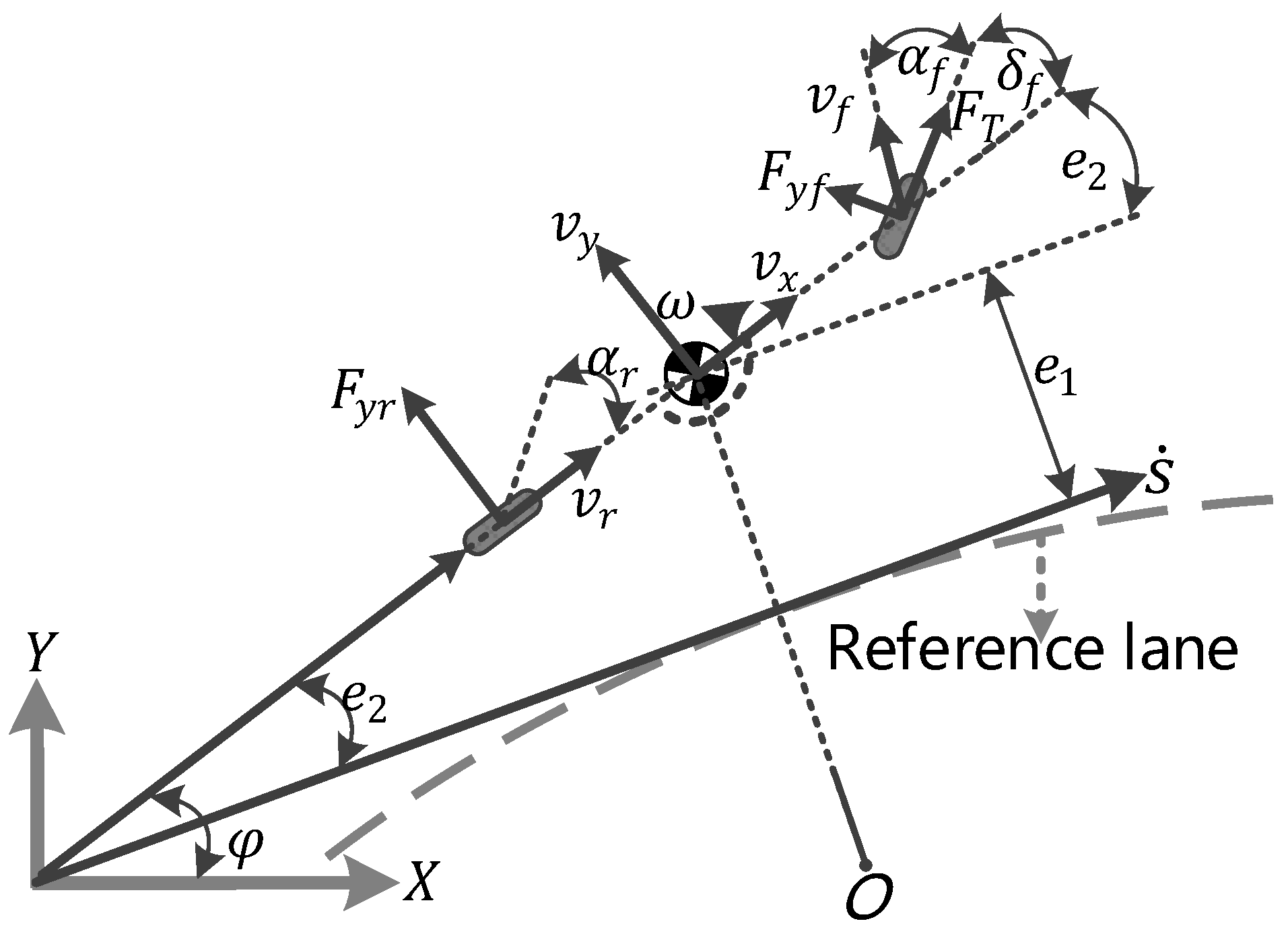
3. Dynamical Model for Motion Planning

According to the analysis results in Section 2, the single-track model only describes the vehicle dynamics when the steering angle of front tire is small, and cannot describe the influence of the force projected from other directions. In this section, the coupling dynamical model (CDM) is established, and then the numerical simplified process is described in detail.

3.1. Longitudinal and Lateral Coupling Model

From the conclusions in Section 2, it is known that in the normal operating range the lateral force of the tire has a linear relationship with the slip angle due to the small lateral acceleration, and the effects of lateral and vertical load transfer can be ignored; thus the vehicle can be considered a rigid body moving on the two-dimensional road surface. The road friction coefficient is an important parameter for dynamic modeling, especially when the longitudinal and lateral acceleration is large. In our statistical results of normal driving conditions, when the vehicle speed was greater than 10 $\mathrm{m}/\mathrm{s}$, the longitudinal and lateral acceleration was relatively small (less than 2.2 ${\mathrm{m}/\mathrm{s}}^2$), so we did not consider the impact of road friction coefficient on vehicle dynamics.

As depicted in Figure 3, $\varphi$ denotes the heading angle, $\omega$ is the yaw rate, $v_x$ and $v_y$ denote the longitudinal and lateral velocities in the vehicle body coordinate $x-y$ respectively. The symbols ${\delta }_f$ and $F_T$ denote the steering angle of front tires and longitudinal driving force, ${\alpha }_f$ and ${\alpha }_r$ denote the slip angle of front and rear tires, $F_{yf}$ and $F_{yr}$ denote the lateral force of front and rear tires, respectively.

According to Newton-Euler equations, the following inertial force balance equations are established [28]:

$$\begin{array}{c}{\dot{v}}_x=\frac{F_T\cos \left({\delta }_f\right)}{m}+\frac{2C_{yf}}{m}\frac{v_y+l_f\omega }{v_x}\sin \left({\delta }_f\right)+v_y\omega -\frac{2C_{yf}}{m}{\delta }_f\sin \left({\delta }_f\right),\hfill \\ {\dot{v}}_y=\frac{F_T\sin \left({\delta }_f\right)}{m}-\frac{2C_{yf}}{m}\frac{v_y+l_f\omega }{v_x}\cos \left({\delta }_f\right)-v_x\omega +\frac{2C_{yf}}{m}{\delta }_f\cos \left({\delta }_f\right)-\frac{2C_{yr}}{m}\frac{v_y-l_r\omega }{v_x},\hfill \\ \hspace{1em}\hspace{1em}\hspace{1em}\hspace{1em}\dot{\omega }=\frac{F_T\sin \left({\delta }_f\right)}{I_z}{l}_f-\frac{2C_{yf}}{I_z}\frac{v_y+l_f\omega }{v_x}\cos \left({\delta }_f\right)l_f+\frac{2C_{yf}}{I_z}{\delta }_f\cos \left({\delta }_f\right)l_f+\frac{2C_{yr}}{I_z}\frac{v_y-l_r\omega }{v_x}{l}_r,\end{array}$$

(1)

where $m$ and $I_z$ are the vehicle mass and inertia, $l_f$ and $l_r$ are the distances from vehicle’s center of gravity to the front and rear axles, $C_{yf}$ and $C_{yr}$ are the cornering stiffness of front and rear tires, respectively. Equation (1) describes both vehicle longitudinal and lateral dynamics, and their coupling effects finely, but it is still complex for application in a model-based motion planner.

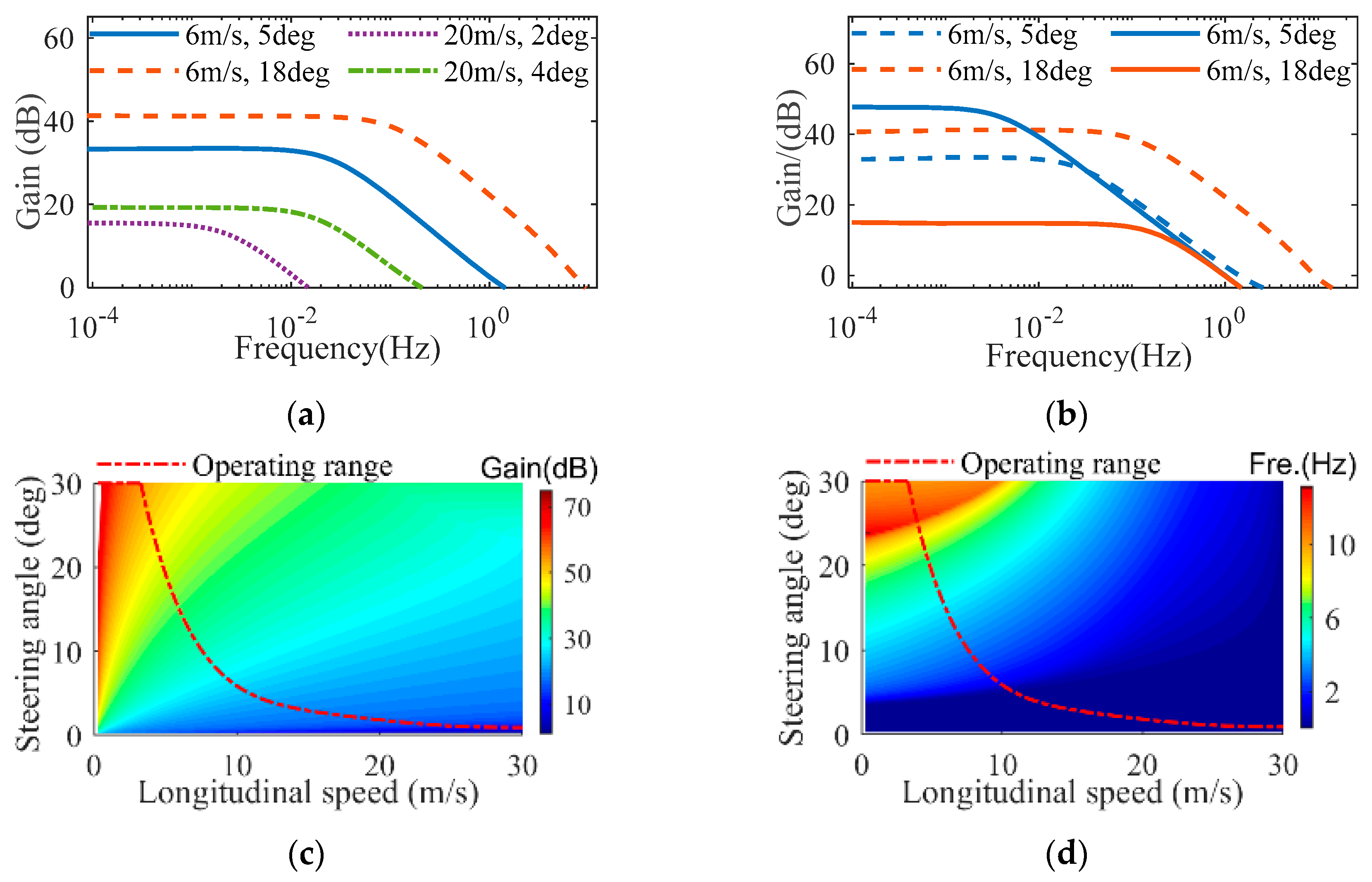
3.2. Simplification of Dynamical Model by Coupling Analysis

In this section, (1) is simplified by numerical analysis of the coupling between lateral and longitudinal dynamics. Let $\mathit{\xi }={\left[v_x{v}_y\omega \right]}^{\mathrm{T}}$ and $\mathit{u}={\left[F_T{\delta }_f\right]}^{\mathrm{T}}$, (1) is written as

$$\dot{\mathit{\xi }}=g\left(\mathit{\xi },\mathit{u}\right).$$

(2)

To reveal the coupling characteristics and simplify the model, it is expanded by the first-order Taylor equation at the equilibrium point, $\left({\mathit{\xi }}_0,{\mathit{u}}_0\right)$ as

$$\Delta \dot{\mathit{\xi }}={\mathit{A}}_{k,0}\Delta \mathit{\xi }+{\mathit{B}}_{k,0}\Delta \mathit{u},$$

(3)

where $\Delta \mathit{\xi }=\mathit{\xi }-{\mathit{\xi }}_0$, $\Delta \mathit{u}=\mathit{u}-{\mathit{u}}_0$, ${\dot{\mathit{\xi }}}_0=\mathit{g}\left({\mathit{\xi }}_0,{\mathit{u}}_0\right)$ and ${\mathit{A}}_{\mathit{k},\mathbf{0}}$ and ${\mathit{B}}_{\mathit{k},\mathbf{0}}$ are the Jacobian matrix of $\mathit{g}\left({\mathit{\xi }}_0,{\mathit{u}}_0\right)$ satisfying:

$${\mathit{A}}_{\mathit{k},\mathbf{0}}={\frac{\mathbf{\partial }\mathit{g}}{\mathbf{\partial }\mathit{\xi }}\mathbf{|}}_{{\mathit{\xi }}_{\mathbf{0}},{\mathit{u}}_{\mathbf{0}}},{\mathit{B}}_{\mathit{k},\mathbf{0}}={\frac{\mathbf{\partial }\mathit{g}}{\mathbf{\partial }\mathit{u}}\mathbf{|}}_{{\mathit{\xi }}_{\mathbf{0}},{\mathit{u}}_{\mathbf{0}}}.$$

(4)

The variation ranges and units of different signals are not the same. For example, the variation range of the vehicle speed is $\left[0,33\right]\mathrm{m}/\mathrm{s}$, while the variation range of the longitudinal force is $\left[-4000,4000\right]\mathrm{N}$. They are normalized firstly to compare the effects on the vehicle dynamics at the same scale. The normalized parameters are selected according to the statistical results in Figure 2 as

$${\overline{v}}_x=30 \mathrm{m}/\mathrm{s},{\overline{F}}_T=m·a\left(v_x\right), {\overline{\delta }}_f=\delta \left(v_x\right),\overline{\omega }=46 \mathrm{deg}/\mathrm{s},$$

(5)

where $a\left(v_x\right)$ and $\delta \left(v_x\right)$ are both look-up table functions with $v_x$ as input. The table data of $a\left(v_x\right)$ is obtained from the 3 $\mathsf{\sigma }$ boundary in Figure 2a and that of $\delta \left(v_x\right)$ is from Figure 2d. The normalized transfer function is

$$\mathit{G}{\left(s\right)}^{\prime }=\left[\begin{array}{cc}\frac{\Delta v_x\left(s\right)}{\Delta F_T\left(s\right)}\ast \frac{{\overline{F}}_T}{{\overline{v}}_x}& \frac{\Delta v_x\left(s\right)}{\Delta {\delta }_f\left(s\right)}\ast \frac{{\overline{\delta }}_f}{{\overline{v}}_x}\\ \frac{\Delta \omega \left(s\right)}{\Delta F_T\left(s\right)}\ast \frac{{\overline{F}}_T}{\overline{\omega }}& \frac{\Delta \omega \left(s\right)}{\Delta {\delta }_f\left(s\right)}\ast \frac{{\overline{\delta }}_f}{\overline{\omega }}\end{array}\right],$$

(6)

where $s$ here represents the Laplacian operator.

In order to analyze the transfer characteristics from ${\delta }_f$ to $v_x$ over the entire operating range, we have calculated the amplitude-frequency characteristics of a total of 22,500 equilibrium points in the range of $v_x\in \left[0,30\right]\mathrm{m}/\mathrm{s}$ and ${\delta }_f\in \left[0,30\right]\mathrm{degree}$ with the step of 0.2. Since the closed-loop system composed of human and vehicle is a low-pass one with a cut-off frequency of less than 1 Hz [31], only the data in the low frequency band was used, for simplicity. The typical amplitude-frequency characteristics are shown in Figure 4a, which are all close to the first-order inertial system. Their open-loop gains and cut-off frequencies at different linearization points are shown in Figure 4c,d, respectively. Both the open-loop gain and cut-off frequency decrease with $v_x$, while increasing with ${\delta }_f$. The minimum open-loop gain is greater than 1 dB, which implies that the lateral input has an obvious effect on the longitudinal dynamics.

To compare the influence of $F_T$ with respect to ${\delta }_f$ on $v_x$, the amplitude-frequency characteristics of $F_T$ to $v_x$ are illustrated in Figure 4b, where ${\delta }_f=5, 18 \mathrm{degree}$. The solid lines are the amplitude-frequency characteristics of $F_T$ to $v_x$, and the dashed lines are that of ${\delta }_f$ to $v_x$. As shown in Figure 4b, ${\delta }_f$ has the same order of the magnitude of the open-loop gain and cut-off frequency as that of $F_T$ on $v_x$, so ${\delta }_f$ has a significant impact on $v_x$.

The same method was also used to analyze the transfer characteristics from $F_T$ to $\omega$, which are shown in Figure 5a when ${\delta }_f=2, 18 \mathrm{degree}$. Their amplitude-frequency characteristics were also close to the first-order inertial system. The open-loop gains are given in Figure 5c, fin which it can be seen that the open-loop gains are negative in most cases and decrease with the increase of ${\delta }_f$ and $v_x$. This implies that the coupling effect of longitudinal input on the lateral dynamics decreases with the increase of ${\delta }_f$ and $v_x$.

To compare the influence of $F_T$ with respect to ${\delta }_f$ on $\omega$, the amplitude-frequency characteristics are shown in Figure 5b when $v_x=6,30\mathrm{m}/\mathrm{s}$. The solid lines are the amplitude-frequency characteristics and the dashed lines are that from $F_T$ to $\omega$. As shown in Figure 5b, $F_T$ has a certain influence on $\omega$ under low-speed, low-frequency and small ${\delta }_f$ operating conditions, but this effect is negligible compared to ${\delta }_f$.

Based on the above analysis, the coupling component of $F_T$ in the lateral dynamics is neglected, and the simplified SDM is obtained from Equation (1):

$$\begin{array}{c}{\dot{v}}_x=\frac{F_T}{m}+\frac{2C_{yf}}{m}\frac{\left(v_y+l_f\omega \right)\sin \left({\delta }_f\right)}{v_x}-\frac{2C_{yf}{\delta }_f\sin \left({\delta }_f\right)}{m}+v_y\omega ,\hfill \\ {\dot{v}}_y=-\frac{2C_{yf}}{m}\frac{\left(v_y+l_f\omega \right)\cos \left({\delta }_f\right)}{v_x}+\frac{2C_{yf}{\delta }_f\cos \left({\delta }_f\right)}{m}-\frac{2C_{yr}}{m}\frac{v_y-l_r\omega }{v_x}-v_x\omega ,\hfill \\ \dot{\omega }=\frac{-2C_{yf}}{I_z}\frac{\left(v_y+l_f\omega \right)\cos \left({\delta }_f\right)l_f}{v_x}+\frac{2C_{yf}{\delta }_f\cos \left({\delta }_f\right)l_f}{I_z}+\frac{2C_{yr}}{I_z}\frac{v_y-l_r\omega }{v_x}{l}_r.\end{array}$$

(7)

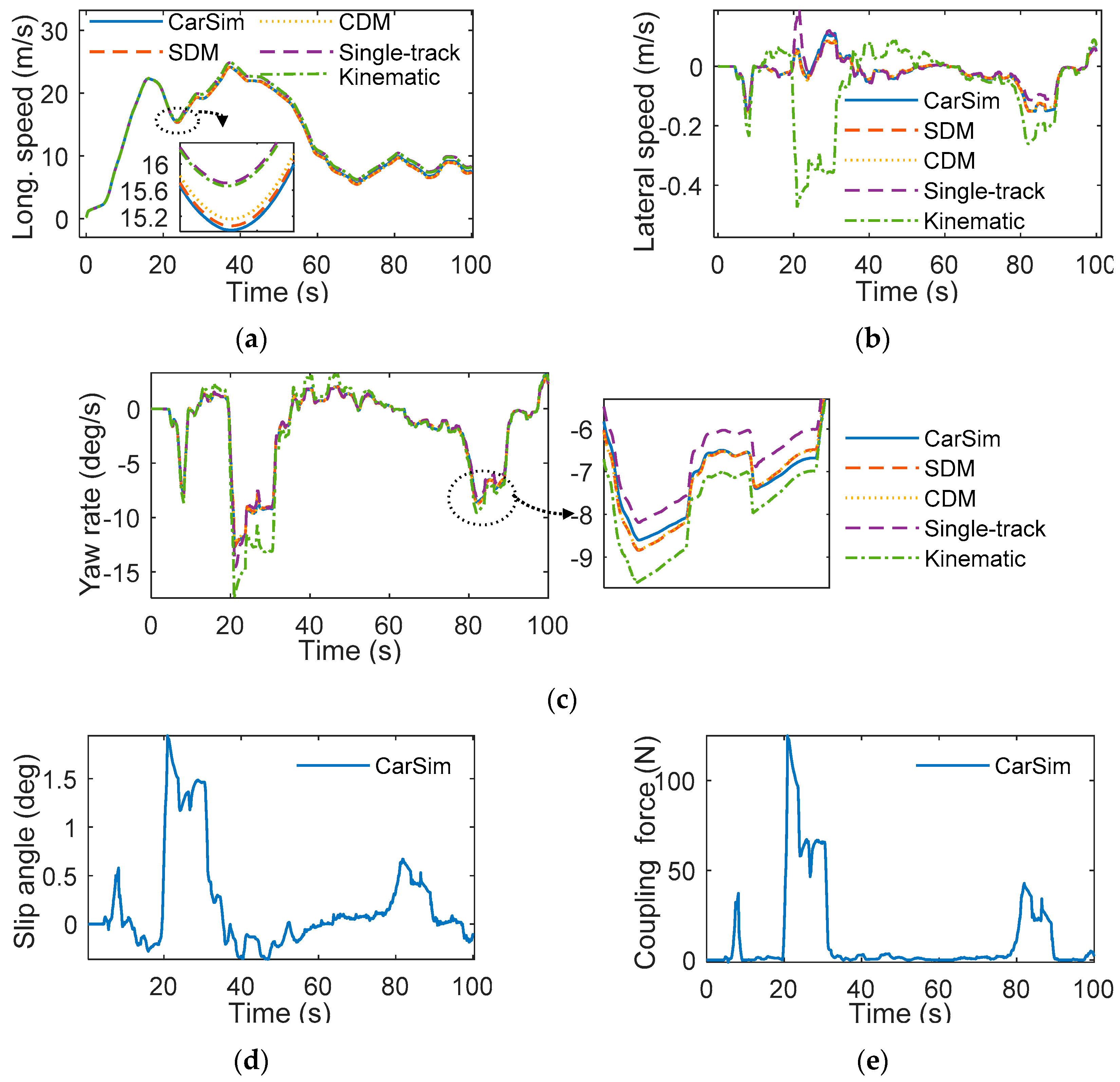
3.3. Validation of Single-Coupled Model

To verify the accuracy of SDM, we have compared it with CDM, the uncoupled single-track model [25], the kinematic model [32], and CarSim [33] by open-loop simulations. In order to reflect the coupling effects, the simulation conditions, containing both acceleration/deceleration, and steering operations, were selected from the FOT data in Section 2. The comparison results were given in Figure 6a–c, in which the single-track model and the kinematic model are denoted by “Single-track” and “Kinematic”, respectively.

Since the lateral coupling force was large in the range of 20–30 s and 80–90 s, as shown in Figure 6e, the single-track model has a large error because it does not consider the dynamical coupling. The kinematic model cannot describe the cornering characteristics of tires, so it also has a large error when the slip angle becomes large at 20–30 s and 80–90 s, as shown in Figure 6d. The proposed SDM can overcome the above shortcomings of the single-track and kinematic models, meanwhile, compared with CDM, SDM has a more concise expression, which is beneficial to the numerical optimization of the motion planning.

4. Motion Planning Application and Analysis

This section constructs motion planning as a closed-loop NMPC problem based on several constraints. Motion planning in emergency conditions is an important problem, and some authors have proposed several effective methods to realize collision avoidance [16]. In this section, we describe the motion planner designed based on SDM to validate the improvement of control performances by considering the dynamical coupling through several comparative HIL tests.

4.1. NMPC Problem Formulation

In order to deal with the constraints of obstacles conveniently, SDM is extended based on the curvilinear coordinate, $s$-$e_1$ [32]:

$$\begin{array}{c}\dot{s}=\frac{1}{1-k{e}_1}·\left(v_x\cos \left(e_2\right)-v_y\sin \left(e_2\right)\right),\\ {\dot{e}}_1=v_x\sin \left(e_2\right)+v_y\cos \left(e_2\right),\\ {\dot{e}}_2=\omega -k\dot{s}.\end{array}$$

(8)

As depicted in Figure 3, $s$ denotes the longitudinal driving distance, $k$ is the curvature of the reference lane, $e_1$ and $e_2$ are the lateral position and heading error with respect to the reference lane, respectively. With the definition of the state $\mathit{x}$, control input $\mathit{u}$ and output $\mathit{y}$ as $\mathit{x}={\left[v_x v_y \omega s e_1 e_2\right]}^{\mathrm{T}}$, $\mathit{u}={\left[F_T {\delta }_f\right]}^{\mathrm{T}}$ and $\mathit{y}={\left[v_x e_1 e_2\right]}^{\mathrm{T}}$, the state function is obtained by combining Equations (7) and (8) together:

$$\dot{\mathit{x}}=f\left(\mathit{x},\mathit{u}\right)=\left[\begin{array}{c}\frac{2C_{yf}\left(v_y+l_f\omega -{\delta }_f{v}_x\right)\sin \left({\delta }_f\right)}{m{v}_x}\\ \frac{2C_{yf}\left({\delta }_f{v}_x-v_y-l_f\omega \right)\cos \left({\delta }_f\right)}{m{v}_x}\\ \frac{2C_{yf}{l}_f\left({\delta }_f{v}_x-v_y-l_f\omega \right)\cos \left({\delta }_f\right)}{I_z{v}_x}\\ 0\\ 0\\ 0\end{array}\right]+\left[\begin{array}{c}\frac{F_T}{m}+v_y\omega \\ \frac{2C_{yr}\left(v_y-l_r\omega \right)}{m{v}_x}-v_x\omega \\ \frac{2C_{yr}\left(v_y-l_r\omega \right)l_r}{I_z{v}_x}\\ \frac{v_x\cos \left(e_2\right)-v_y\sin \left(e_2\right)}{1-k{e}_1}\\ v_x\sin \left(e_2\right)+v_y\cos \left(e_2\right)\\ \omega -k\dot{s}\end{array}\right]$$

(9)

NMPC motion planning needs to solve a nonlinear program at each sampling instant. The finite-dimensional discrete nonlinear program for it is

$$\underset{\mathit{X},\mathit{U}}{\min }{\displaystyle \sum }_{i=0}^{N-1}\frac{\Vert {\mathit{y}}_i-{\mathit{y}}_{des}\Vert {}_{\mathit{Q}}^2+\Vert {\mathit{u}}_i\Vert {}_{\mathit{P}}^2+\Vert \Delta {\mathit{u}}_i\Vert {}_{\mathit{R}}^2+{\rho }_{ϵ}{ϵ}_i{}^2}{2},$$

(10)

$$\mathrm{s}.\mathrm{t}.\mathit{x}\left(0\right)={\mathit{x}}_0,$$

(11)

$${\mathit{x}}_{i+1}=f\left({\mathit{x}}_i,{\mathit{u}}_i\right),\hspace{1em}i=0,\dots ,N-1,$$

(12)

$${\left(\frac{e_{1,i}-e_{ovj,i}}{a_{j,i}}\right)}^2+{\left(\frac{s_i-s_{ovj,i}}{b_{j,i}}\right)}^2+ϵ\ge 1,$$

(13)

$$0\le v_{x,i}\le {\overline{v}}_{x,i},\hspace{1em}i=0,\dots ,N,$$

(14)

$${\underset{\_}{e}}_{1,i}\le e_{1,i}\le {\overline{e}}_{1,i}, i=0,\dots ,N,$$

(15)

$$-\overline{{\mathit{u}}_i}\le {\mathit{u}}_i\le \overline{{\mathit{u}}_i}, i=0,\dots ,N-1,$$

(16)

$$-\mathbf{\Delta }\overline{{\mathit{u}}_i}\le \mathbf{\Delta }{\mathit{u}}_i\le \mathbf{\Delta }\overline{{\mathit{u}}_i},i=0,\dots ,N-1,$$

(17)

$$0\le {ϵ}_i\le 1$$

(18)

where $\mathit{X}={\left[{\mathit{x}}_{\mathbf{0}}{}^{\mathrm{T}}\dots {\mathit{x}}_{\mathit{N}}{}^{\mathrm{T}}\right]}^{\mathrm{T}}$, $\mathit{U}={\left[{\mathit{u}}_{\mathbf{0}}{}^{\mathrm{T}}{ϵ}_0\dots {\mathit{u}}_{\mathit{N}}{}^{\mathrm{T}}{ϵ}_N\right]}^{\mathrm{T}}$, and ${\mathit{y}}_{des}={\left[v_{xdes} e_{1des} 0\right]}^{\mathrm{T}}$.

This optimization problem is defined over the predictive horizon $T$ with the predictive step size $N$. The cost function Equation (10) consists of the tracking performance, the control efforts, the change rates of control and the slack variable. The symbols $\mathit{Q}$, $\mathit{P}$, and $\mathit{R}$ are the positive semi-definite weighting matrices. Equation (12) represents the discrete form of vehicle dynamical model, i.e., SDM, the single-track or kinematic model, which are obtained by the multiple shooting discretization method [34]. About the discretization, the forward Euler integrator was used and the step was 0.05 s. The discretization error of multiple shooting and the computational complexity of NMPC have been studied in [22], and [35]. This nonlinear program depends on the current state ${\mathit{x}}_0\in {ℝ}^{n_{\mathit{x}}}$. Inequality Equation (13) is the spatiotemporal elliptical constraint of the j-th obstacle. The symbols $e_{ovj,i}$ and $s_{ovj,i}$ are the lateral position and longitudinal distance of the j-th obstacle. The minor axis $a_{j,i}$ and major axis $b_{j,i}$ of the ellipse are determined by the size of the subject vehicle and the obstacles, as well as the relative speed. The larger the size and relative speed of the obstacles and subject vehicle are, the larger the ellipse becomes. Detailed information about the spatiotemporal elliptical constraint can be found in [32]. The slack variable $ϵ$ relaxes the constraint to prevent the infeasibility. In Equation (14), ${\overline{v}}_{x,i}$ is the maximum speed. In Equation (15), ${\overline{e}}_{1,i}$ and ${\underset{\_}{e}}_{1,i}$ are the constraints of road. Equations (16) and (17) are constraints of the limitation of vehicle performance and actuators. In ${\mathit{y}}_{des}$, $v_{xdes}$ is the desired speed, $e_{1des}$ is the lateral distance from the center of lane to the vehicle’s center of gravity.

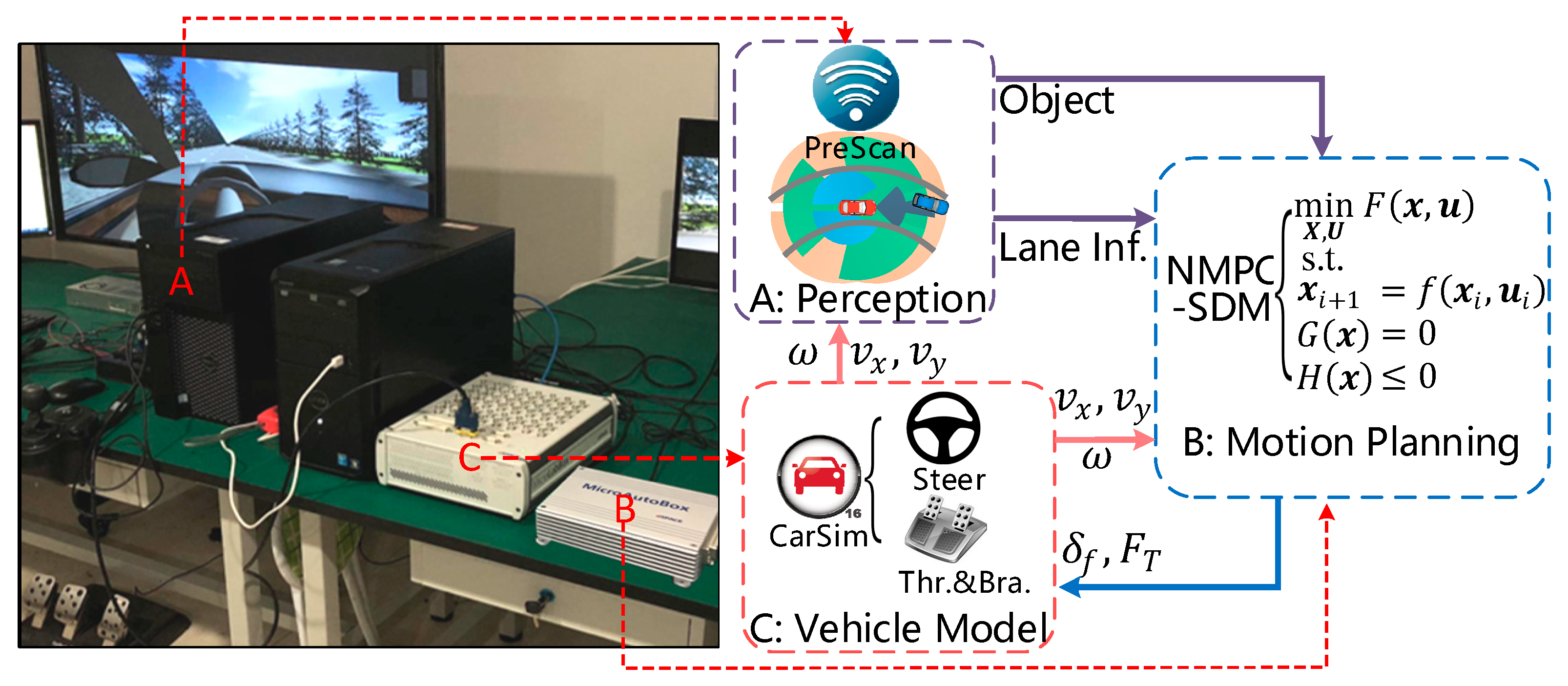
4.2. Platform for HIL Test

The HIL platform is shown in Figure 7.

As shown in Figure 7, the HIL is mainly composed of three parts: perception module “A”; motion planner “B”; and vehicle model “C” [36]. These modules communicate with each other via a control area network. The virtual reality simulation software “PreScan” runs on “A”, which is a graphics workstation. It is used to simulate the traffic environment (object, lane etc.) and visualize the vehicle states. The module “B” is a rapid prototype controller produced by dSPACE and called “MicroAutoBox II” (Quad-core ARM A57 CPU, 2 GHz, and 256-core NVIDIA Pascal GPU). The NMPC algorithm was implemented in it and solved by sequential quadratic programming (SQP) with the real-time iterative framework [37]. The close-loop stability and recursive feasibility were proven in [37]. To obtain a real-time feasibility, the code generation tool, CasADi [38], combined with the quadratic programming solver, qpOASES [39], were used to generate the efficient C-code. The operation cycle was 0.05 s. The module “C” is the real-time simulator of dSPACE called “MicroLabBox”, in which CarSim runs. In module “C”, the driving force is converted into throttle angle ${\alpha }_{thr}$ and braking pressure $P_{brk}$ through the vehicle longitudinal inverse dynamics model [40], and the steering angle of front tire is converted into steering wheel angle ${\delta }_w$ through the coefficient of the steering system. The converted throttle, brake and steering wheel angle are used as inputs to CarSim.

The pseudo-code for the NMPC-SDM algorithm is shown in Algorithm 1.

Algorithm 1 Outputs: Throttle ${\alpha }_{thr}$, brake $P_{brk}$, steering wheel angle ${\delta }_w$

1: Inputs: ${\mathit{x}}_0$, $e_{ovj,i}$ and $s_{ovj,i}$, $a_{j,i}$ and $b_{j,i}$

2: while true do

3: $\mathit{U}=\left[{\mathit{u}}_{\mathbf{0}}{}^{\mathrm{T}},\dots ,{\mathit{u}}_{\mathit{N}}{}^{\mathrm{T}}\right]$, $t_s=0.05$$\leftarrow$Initialization of control vector $\mathit{U}$ and discretization step $t_s$.

4: $\mathit{X}={\left[{\mathit{x}}_{\mathbf{0}}{}^{\mathrm{T}}\dots {\mathit{x}}_{\mathit{N}}{}^{\mathrm{T}}\right]}^{\mathrm{T}}\leftarrow$Using $\mathit{U}$as control input vector, ${\mathit{x}}_{\mathbf{0}}$ as initial state, discretization state function (9) with multiple shooting in all shooting intervals $i$ to obtain the states vector $\mathit{X}$.

5: Prepare the nonlinear program Equations (10)–(18) with $\mathit{X}$ and $\mathit{U}$ as optimization variables.

6: ${\mathit{U}}^{\ast }={\left[{\mathit{u}}_0^{\ast }{}^{\mathrm{T}}{ϵ}_0^{\ast }\dots {\mathit{u}}_N^{\ast }{}^{\mathrm{T}}{ϵ}_N^{\ast }\right]}^{\mathrm{T}}\leftarrow$Using SQP with real-time iterative framework to solve the nonlinear program, and the optimal control vector ${\mathit{U}}^{\ast }$ is obtained.

7: Send ${\mathit{u}}_0^{\ast }$ to the inverse vehicle dynamics model.

8: Calculate ${\alpha }_{thr}$, $P_{brk}$ and ${\delta }_w$.

9: end while

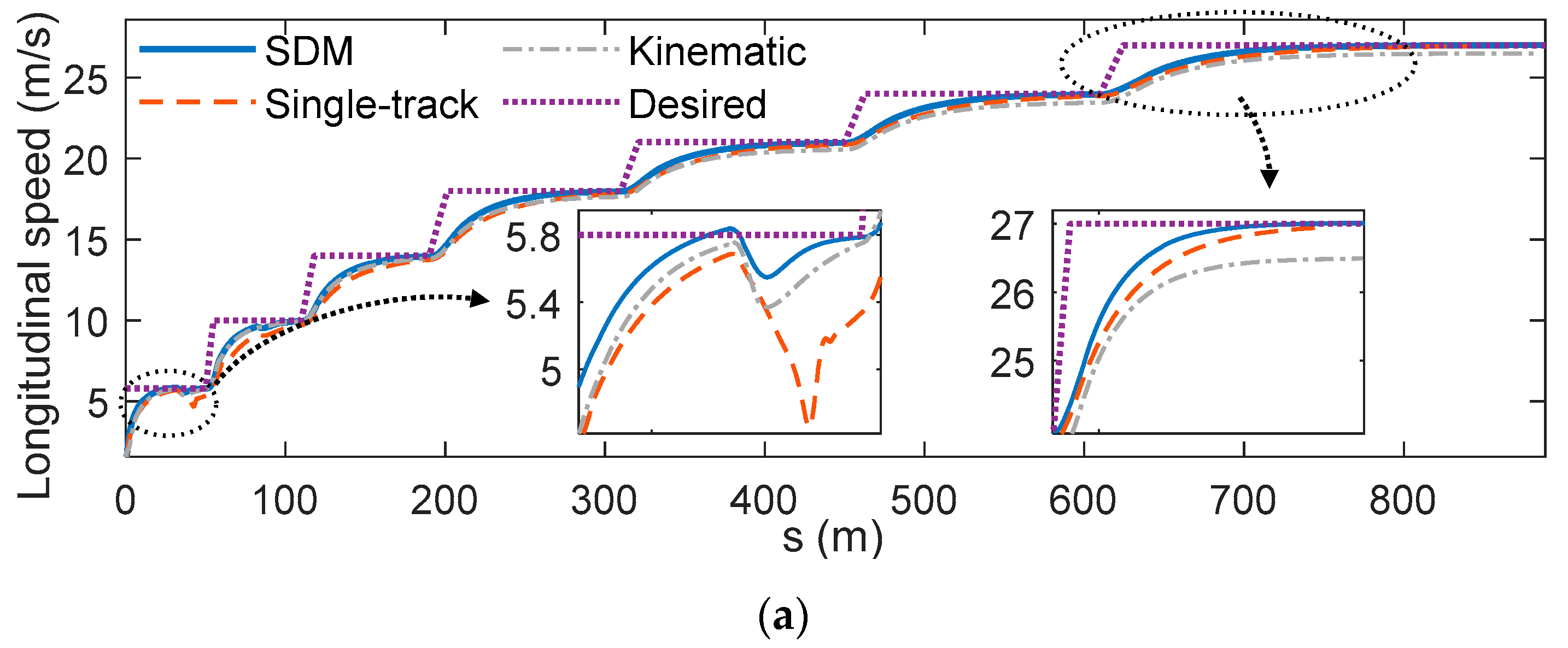
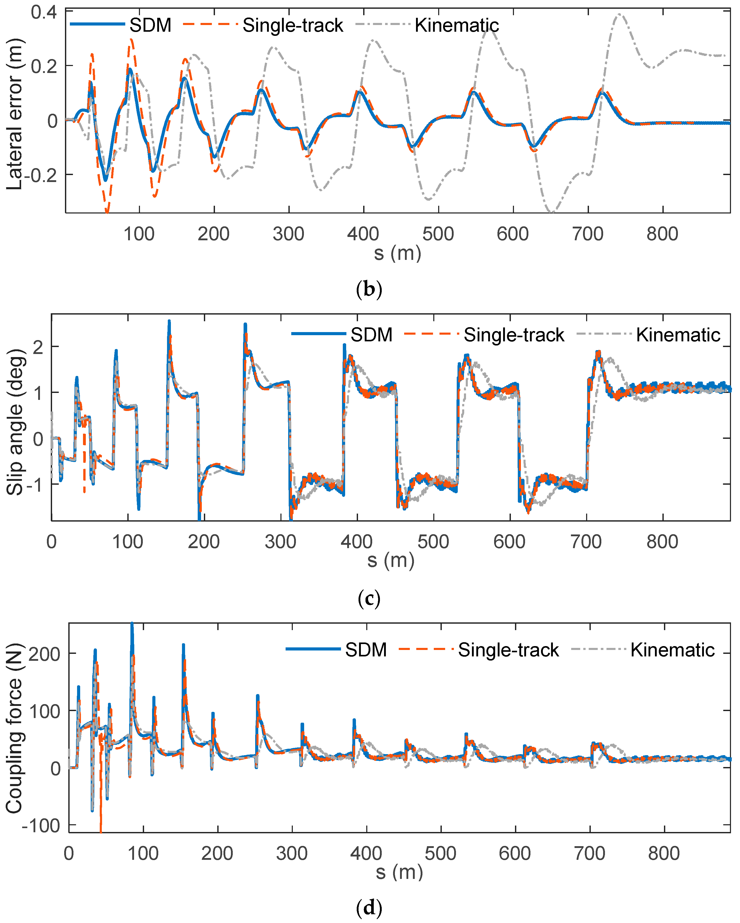
4.3. Experimental Results and Analysis

The parameters of the vehicle model and NMPC are presented in

Table 1. Parameters of dynamical model and nonlinear program.

Symbol	Value	Symbol	Value
$l_f$	$1.17\mathrm{m}$	$Q$	$\mathrm{diag}\left(0.844,1,40\right)$
$l_r$	$1.77\mathrm{m}$	$P$	$\mathrm{diag}\left({10}^{-5}, 62.5\right)$
$C_{yf}$	$\mathrm{54,600}\mathrm{N}/\mathrm{rad}$	$R$	$\mathrm{diag}\left({10}^{-4},90\right)$
$C_{yr}$	$\mathrm{54,600}\mathrm{N}/\mathrm{rad}$	${\rho }_{ϵ}$	$500$
$I_z$	$1943\mathrm{kg}·{\mathrm{m}}^2$	${\underset{\_}{v}}_x,{\overline{v}}_x$	$0,33.3\mathrm{m}/\mathrm{s}$
$m$	$1460\mathrm{kg}$	${\underset{\_}{e}}_1,{\overline{e}}_1$	$-1.875\mathrm{m},5.625\mathrm{m}$
$N$	$60$	$\overline{u}$	${\left[4000 \mathrm{N} \delta \left(v_x\right) \mathrm{deg}\right]}^{\mathrm{T}}$
$T$	$3\mathrm{s}$	$\Delta \overline{u}$	${\left[4000\mathrm{N}/\mathrm{s}63\mathrm{deg}/\mathrm{s}\right]}^{\mathrm{T}}$

.

To verify the improvement of the motion planning performances by considering the dynamical coupling, the driving scenarios with strong coupling were preferred, such as cruising on a curved road, lane changing, and so on:

(1)

SCENARIO 1 was designed to verify the effectiveness of NMPC-SDM when the vehicle is cruising on an S-shaped road. It consists of continuous bends with decreasing curvature and increasing desired speed, as illustrated in Figure 8 and Figure 9a.

(2)

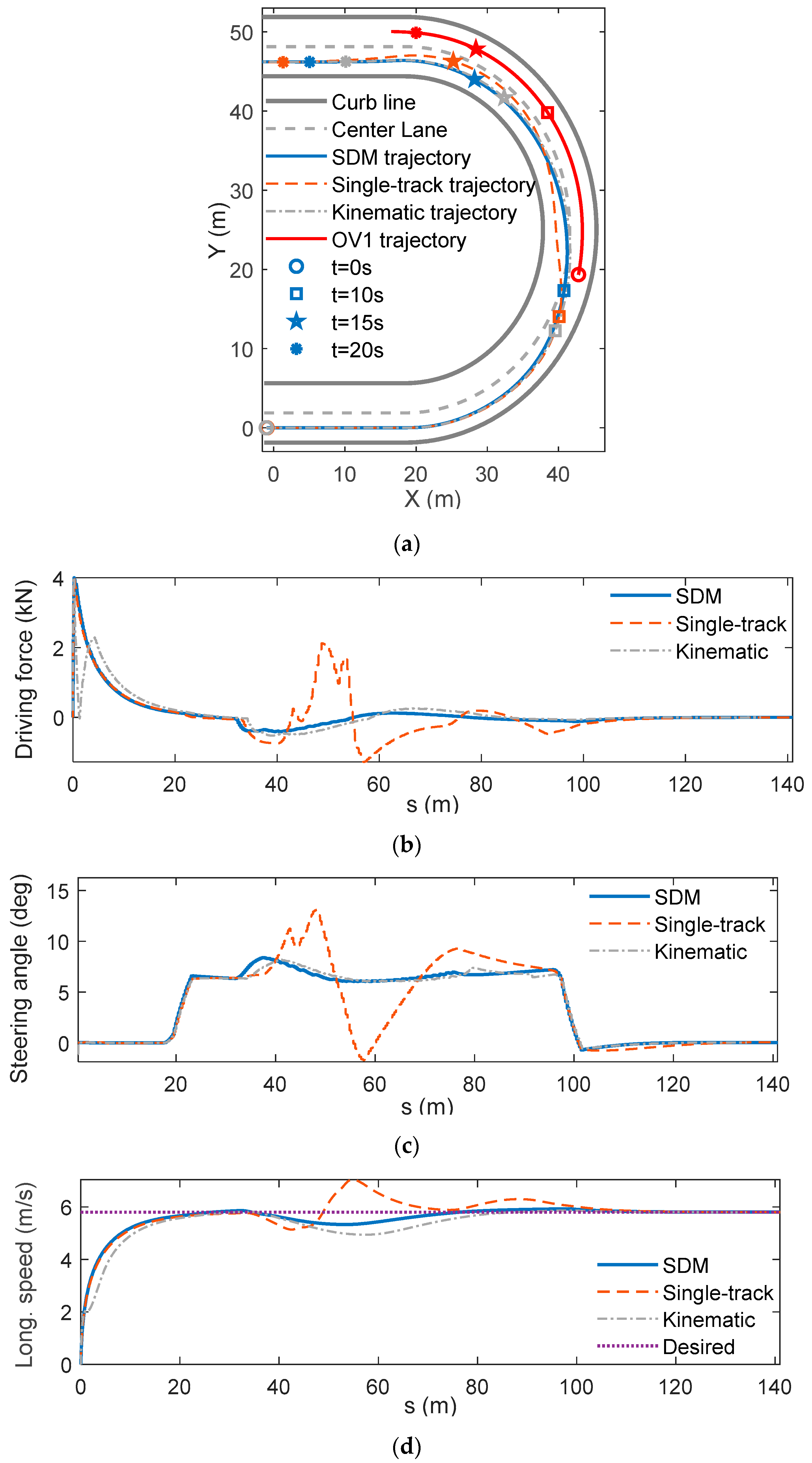
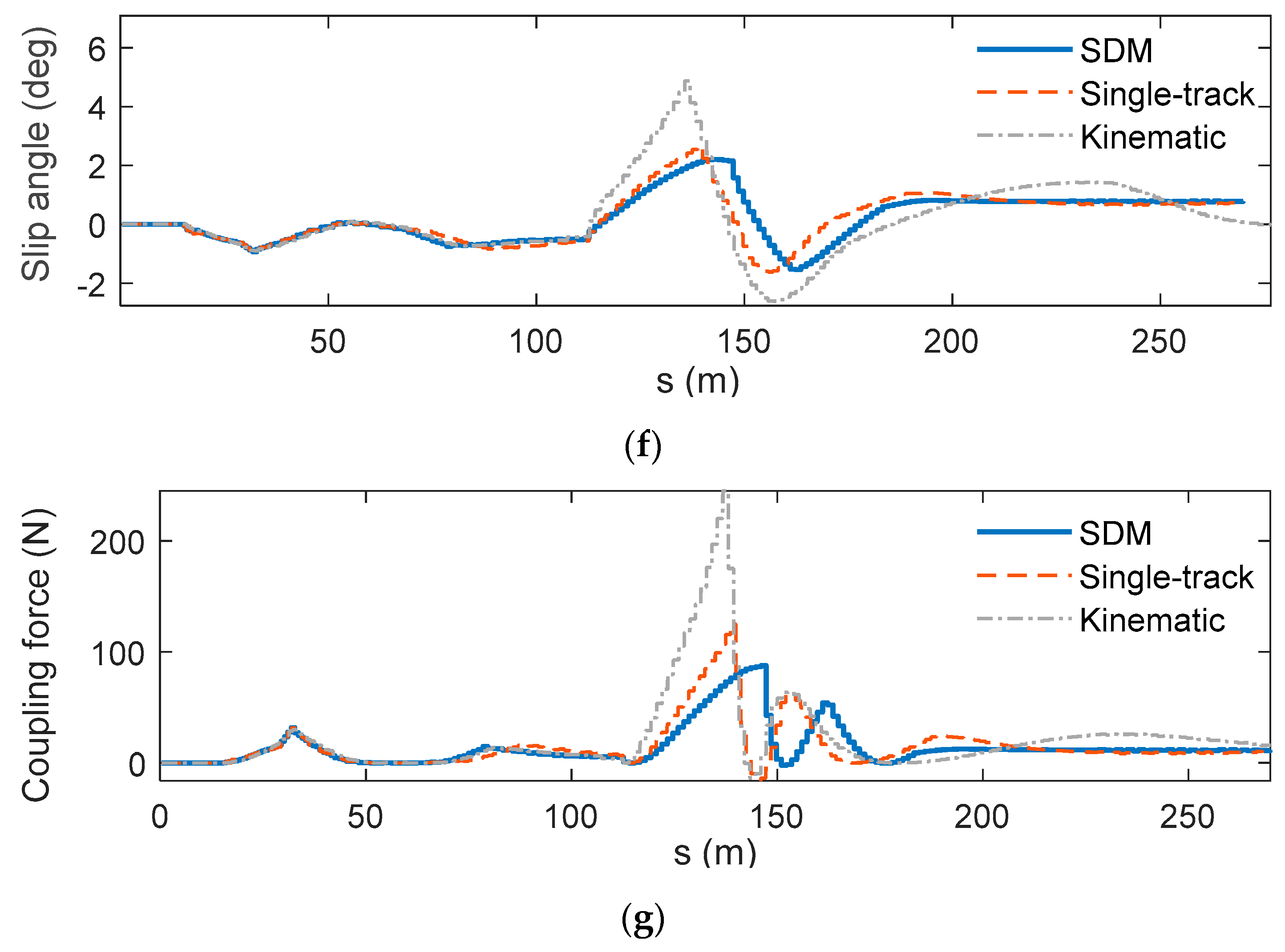
SCENARIO 2 verifies the effectiveness of NMPC-SDM when the vehicle makes a lane change in a U-turn with low speed, as shown in Figure 10a. It consists of two $20\mathrm{m}$ straight roads at the start and the end, and an $80\mathrm{m}$ bend in the middle (Curvature of the bend is $0.04{\mathrm{m}}^{-1}$). An obstacle vehicle denoted by OV1 drives along the right lane.

(3)

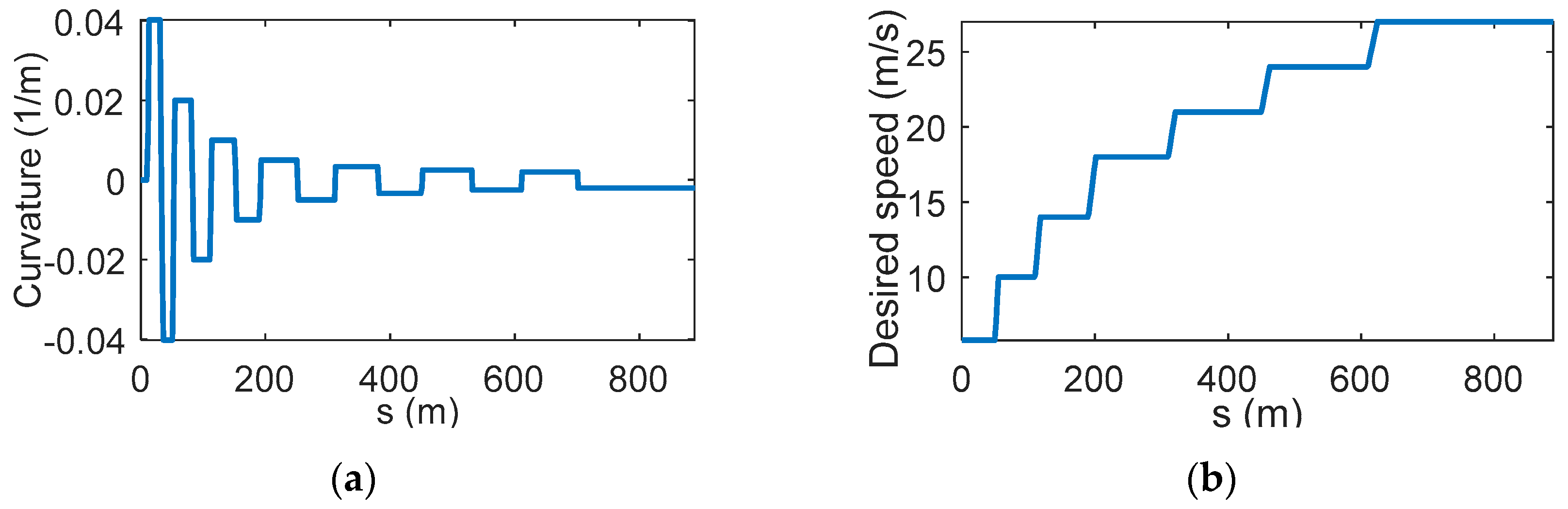
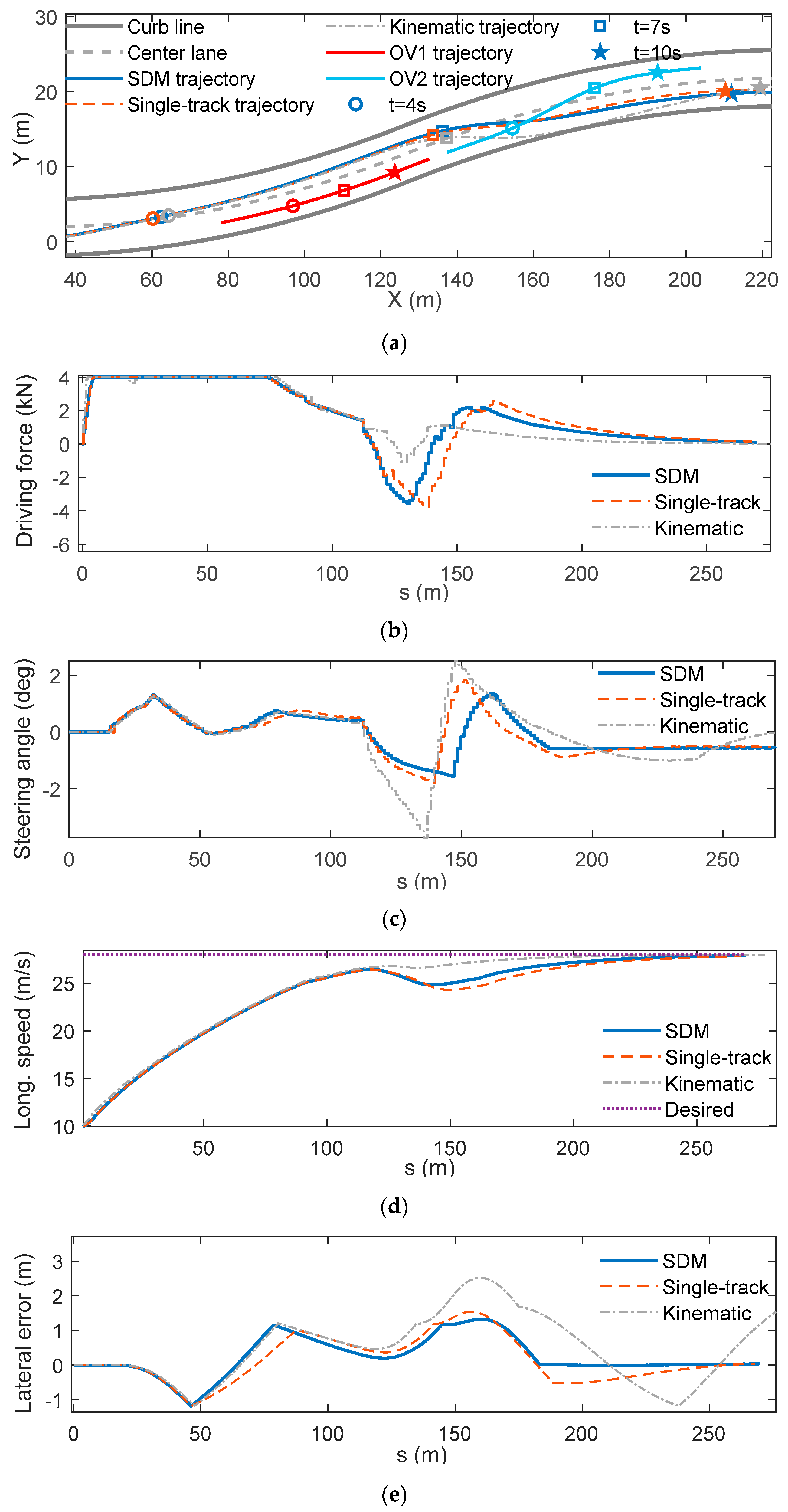
SCENARIO 3 is an overtaking process with high speed on several successive bends as shown in Figure 11a.

It consisted of a $30\mathrm{m}$ straight road, a $100\mathrm{m}$ counter-clockwise bend and a $100\mathrm{m}$ clockwise bend (Curvature of both bends is $0.002{\mathrm{m}}^{-1}$). Obstacle 1, denoted by OV1, ran along the right lane and obstacle 2, denoted by OV2, cut into the left lane from the right.

The roads in SCENARIO 2 and 3 were composed of two lanes, whose parameters are shown in

Table 2. Road parameters of SCENARIO 2 and 3.

No.	Initial Speed	Desired Speed	Obstacle
2	0	$5.8\mathrm{m}/\mathrm{s}$	OV1: $s_{ov1}=55\mathrm{m}$, $v_{ov1}=3\mathrm{m}/\mathrm{s}$.
3	$10\mathrm{m}/\mathrm{s}$	$28\mathrm{m}/\mathrm{s}$	OV1: $s_{ov1}=80\mathrm{m}$, $v_{ov1}=3\mathrm{m}/\mathrm{s}$; OV2: $s_{ov2}=140\mathrm{m}$, $v_{ov2}=10\mathrm{m}/\mathrm{s}$.

.

SCENARIO 3 was the most complicated one among the three scenarios, which included two dynamical obstacles. When the scenario became more complex, such as overtaking with multi-obstacles, complex urban scenario and so on, the constraint number of obstacle in Equation (13) increased. The proposed planner can also be applied to more complicated driving situations. Here we focus on the validation of the improvement of planning performances by considering the coupling between lateral and longitudinal dynamics.

The experimental results from SCENARIO 1–3 are given in Figure 9, Figure 10 and Figure 11, respectively. In each figure, the solid lines are the results of NMPC-SDM (denoted by “SDM”), the dashed lines are the results of NMPC-single-track model (denoted by “Single-track”), and the dash-dotted lines are the results of NMPC-kinematic model (denoted by “Kinematic”).

Since there was no obstacle vehicle in SCENARIO 1, the subject vehicle (SV) runs with the maximum speed in the center of lane. During the low-speed stage with a larger curvature, i.e., $s\in \left[0,80\right] \mathrm{m}$, the longitudinal coupling component of lateral force was large (which the peak reaches 252 N as shown in Figure 9d) and the tracking performance of the single-track model based planner was worse (See Figure 9a,b). As shown in Figure 9c, with the increase of the speed and the decrease of the curvature, the lateral force in the longitudinal direction became smaller gradually, but the slip angle increased. This results in a gradual increase of the control error of the kinematic model-based planner, which the peak reached 0.39 m. However, the control error of the single-track model-based planner decreased gradually. Based on the above results, it can be seen that the kinematic model based planner performed poorly under high-speed conditions, where the slip angle of the tire was over 1.6 degree, and the single-track model-based planner performed poorly under low-speed and large steering angle conditions, in which the coupling force is over 130 N. Because SDM takes into account both dynamical coupling and tire cornering characteristics, NMPC-SDM exhibited better performance than other two planners.

In SCENARIO 2, SV started from the initial position in the right lane. Since there was a low-speed obstacle in the same lane, SV changed to the adjacent lane and then performed lane keeping. The results in Figure 10a show that all planners could successfully complete the lane change. In Figure 10b,c, the control commands of the single-track model-based planner oscillates within the range of $s\in \left[40,80\right]\mathrm{m}$ and has large longitudinal and lateral control errors as shown in Figure 10d,e. This is caused by the large coupling force, as illustrated in Figure 10g, which reaches 500 N. The single-track model didn’t consider this coupling effect. Furthermore, it can be seen in Figure 10f that the tire’s slip angle was small (the absolute value less than 1.2 degrees). Therefore, the performance of the kinematic model-based planner was similar to NMPC-SDM.

In SCENARIO 3, since OV1 was in front of SV with a low speed, SV changed to the left lane. At the same time, OV2 cut into the left lane from the right, so SV changed to the right immediately. In Figure 11a, it can be seen that both NMPC-SDM and the single-track model-based planner could successfully overtake and finally return to the middle of the lane. It can be seen in Figure 11g that the dynamical coupling effect was weak (the peak of SDM is less than 85 N) due to the small steering angle required to overtake. Therefore, the planning results of the two planners were consistent, as compared in Figure 11b,c. However, as shown in Figure 11f, because of the large slip angle of the tire, which reached 5 degrees, the prediction error of the kinematic model was large. This resulted in a collision with the curb and large longitudinal/lateral control errors, as shown in Figure 11d,e.

To verify the real-time performance of the proposed algorithm, we took SCENARIO 3 as an example to show the execution time of solving NMPC in Figure 12. Among the four planners, NMPC-kinematic had the shortest execution time, while NMPC-CDM had the longest execution time. The execution time of NMPC-SDM was shorter than that of NMPC-CDM, especially when SV approached the obstacles. The average execution time of NMPC-SDM and NMPC-CDM was 0.037 s and 0.041 s, respectively. It can be seen that the simplification of the dynamic model reduced the average execution time of the planner by 9.6%. Therefore, we conclude that the simplification of the model can reduce the complexity of the NMPC.

5. Conclusions

This paper investigates the coupling of longitudinal and lateral dynamics for motion planning of autonomous vehicles in normal driving. According to the numerical analyses and validation results, the following conclusions were drawn:

(1)

In order to predict vehicle states accurately, especially in the conditions with low-speed and large steering angle, the coupling effect between the lateral and longitudinal dynamics is not negligible;

(2)

The SDM proposed in this paper can characterize the vehicle longitudinal and lateral dynamical coupling effect and achieve a good balance between the accuracy and complexity;

(3)

Compared with the kinematic and single-track model-based planners, the proposed NMPC-SDM planner improves the performance of motion planning in normal driving.

In the future work, the proposed framework will be validated under more challenging scenarios, such as obstacle avoidance with multiple obstacles, overtaking under uncertain disturbances, and so on. Moreover, field testing should be carried out to verify the effectiveness of the algorithm in real traffic environments.

References

1. Li, K.; Li, S.; Gao, F.; Lin, Z.; Li, J.; Sun, Q. Robust Distributed Consensus Control of Uncertain Multi-Agents Interacted by Eigenvalue-Bounded Topologies. IEEE Internet Things J. 2020. [Google Scholar] [CrossRef]
2. Zhang, J.; Wang, F.; Wang, K.; Lin, W.; Xu, X.; Chen, C. Data-Driven Intelligent Transportation Systems: A Survey. IEEE Trans. Intell. Transp. Syst. 2011, 12, 1624–1639. [Google Scholar] [CrossRef]
3. Watzenig, D.; Horn, M. Automated Driving: Safer and More Efficient Future Driving; Springer: London, UK, 2016; pp. 3–17. [Google Scholar]
4. Schwarting, W.; Alonso-Mora, J.; Rus, D. Planning and Decision-Making for Autonomous Vehicles. Annu. Rev. Control Robot. Auton. Syst. 2018, 1, 187–210. [Google Scholar] [CrossRef]
5. Paden, B.; Čáp, M.; Yong, S.; Yershov, D.; Frazzoli, E. A Survey of Motion Planning and Control Techniques for Self-Driving Urban Vehicles. IEEE Trans. Intell. Veh. 2016, 1, 33–55. [Google Scholar] [CrossRef] [Green Version]
6. González, D.; Pérez, J.; Milanés, V.; Nashashibi, F. A Review of Motion Planning Techniques for Automated Vehicles. IEEE Trans. Intell. Transp. Syst. 2016, 17, 1135–1145. [Google Scholar] [CrossRef]
7. Katrakazas, C.; Quddus, M.; Chen, W.H. Real-time motion planning methods for autonomous on-road driving: State-of-the-art and future research directions. Trans. Res. Part C Emerg. Technol. 2015, 60, 416–442. [Google Scholar] [CrossRef]
8. Khatib, O. Real-Time Obstacle Avoidance for Manipulators, and Mobile Robots. Int. J. Robot. Res. 1985, 5, 90–98. [Google Scholar] [CrossRef]
9. Lee, K.; Kum, D. Collision Avoidance/Mitigation System: Motion Planning of Autonomous Vehicle via Predictive Occupancy Map. IEEE Access 2019, 7, 52846–52857. [Google Scholar] [CrossRef]
10. Huang, Y.; Ding, H.; Zhang, Y.; Wang, H.; Cao, D.; Xu, N.; Hu, C. A Motion Planning and Tracking Framework for Autonomous Vehicles Based on Artificial Potential Field Elaborated Resistance Network Approach. IEEE Trans. Ind. Electron. 2020, 67, 1376–1386. [Google Scholar] [CrossRef]
11. LaValle, S.M. Planning Algorithms; Cambridge University Press: Cambridge, UK, 2006; pp. 85–117. [Google Scholar]
12. Zhang, C.; Chu, D.; Liu, S.; Deng, Z.; Wu, C.; Su, X. Trajectory Planning and Tracking for Autonomous Vehicle Based on State Lattice and Model Predictive Control. IEEE Intell. Transp. Syst. Mag. 2019, 11, 29–40. [Google Scholar] [CrossRef]
13. Kuwata, Y.; Teo, J.; Fiore, G.; Karaman, S.; Frazzoli, E.; How, J.P. Real-Time Motion Planning with Applications to Autonomous Urban Driving. IEEE Trans. Control Syst. Technol. 2009, 17, 1105–1118. [Google Scholar] [CrossRef]
14. Karaman, S.; Frazzoli, E. Sampling-Based Algorithms for Optimal Motion Planning. Int. J. Robot. Res. 2011, 30, 846–894. [Google Scholar] [CrossRef]
15. Chen, L.; Shan, Y.; Tian, W.; Li, B.; Cao, D. A Fast and Efficient Double-Tree RRT-Like Sampling-Based Planner Applying on Mobile Robotic Systems. IEEE/ASME Trans. Mech. 2018, 23, 2568–2578. [Google Scholar] [CrossRef]
16. Liu, J.; Jayakumar, P.; Stein, J.L.; Ersal, T. Combined Speed and Steering Control in High-Speed Autonomous Ground Vehicles for Obstacle Avoidance Using Model Predictive Control. IEEE Trans. Veh. Technol. 2017, 66, 8746–8763. [Google Scholar] [CrossRef]
17. Chen, J.; Zhan, W.; Tomizuka, M. Autonomous Driving Motion Planning with Constrained Iterative LQR. IEEE Trans. Intell. Veh. 2019, 4, 244–254. [Google Scholar] [CrossRef]
18. Gao, Y. Model Predictive Control for Autonomous and Semi-Autonomous Vehicles. Ph.D. Thesis, Department Engineering Mechanical Engineering, University of California, Berkeley, CA, USA, 2014. [Google Scholar]
19. Gao, F.; Lin, F.; Liu, B. Distributed Hinf Control of Platoon Interacted by Switching and Undirected Topology. Int. J. Autom. Technol. 2020, 21, 259–268. [Google Scholar] [CrossRef]
20. Li, B.; Zhang, Y.; Shao, Z.; Jia, N. Simultaneous Versus Joint Computing: A Case Study of Multi-Vehicle Parking Motion Planning. J. Comput. Sci. 2017, 20, 30–40. [Google Scholar] [CrossRef]
21. Rastgoftar, H.; Zhang, B.; Atkins, E.M. A Data-Driven Approach for Autonomous Motion Planning and Control in Off-Road Driving Scenarios. In Proceedings of the American Control Conference (ACC), Milwaukee, WI, USA, 27–29 June 2018; pp. 5876–5883. [Google Scholar]
22. Kong, J.; Pfeiffer, M.; Schildbach, G.; Borrelli, F. Kinematic and Dynamic Vehicle Models for Autonomous Driving Control Design. In Proceedings of the IEEE Intelligent Vehicles Symposium (IV), Seoul, Korea, 28 June–1 July 2015; pp. 1094–1099. [Google Scholar]
23. Ma, C.; Xue, J.; Liu, Y.; Yang, J.; Li, Y.; Zheng, N. Data-Driven State-Increment Statistical Model and Its Application in Autonomous Driving. IEEE Trans. Intell. Transp. Syst. 2018, 19, 3872–3882. [Google Scholar] [CrossRef]
24. Carvalho, A.; Gao, Y.; Gray, A.; Tseng, H.E.; Borrelli, F. Predictive Control of An Autonomous Ground Vehicle Using An Iterative Linearization Approach. In Proceedings of the IEEE Conference on Intelligent Transportation Systems (ITSC 2013), Hague, The Netherlands, 6–9 October 2013; pp. 2335–2340. [Google Scholar]
25. Wang, H.; Huang, Y.; Khajepour, A.; Zhang, Y.; Rasekhipour, Y.; Cao, D. Crash Mitigation in Motion Planning for Autonomous Vehicles. IEEE Trans. Intell. Trans. Syst. 2019, 20, 3313–3323. [Google Scholar] [CrossRef]
26. Betz, J.; Wischnewski, A.; Heilmeier, A.; Nobis, F.; Hermansdorfer, L.; Stahl, T.; Herrmann, T.; Lienkamp, M. A Software Architecture for the Dynamic Path Planning of an Autonomous Racecar at the Limits of Handling. In Proceedings of the IEEE International Conference on Connected Vehicles and Expo (ICCVE 2019), Graz, Austria, 4–8 November 2019; pp. 1–8. [Google Scholar]
27. Stahl, T.; Wischnewski, A.; Betz, J.; Lienkamp, M. Multilayer Graph-Based Trajectory Planning for Race Vehicles in Dynamic Scenarios. In Proceedings of the IEEE Intelligent Transportation Systems Conference (ITSC 2019), Auckland, New Zealand, 27–30 October 2019; pp. 3149–3154. [Google Scholar]
28. Rajamani, R. Vehicle Dynamics and Control; Springer: New York, NY, USA, 2012; pp. 15–87. [Google Scholar]
29. Liu, J.; Jayakumar, P.; Stein, J.L.; Ersal, T. A Study on Model Fidelity for Model Predictive Control-Based Obstacle Avoidance in High-Speed Autonomous Ground Vehicles. Veh. Syst. Dyn. 2016, 54, 1629–1650. [Google Scholar] [CrossRef]
30. Wang, W.; Liu, C.; Zhao, D. How Much Data are Enough? A Statistical Approach With Case Study on Longitudinal Driving Behavior. IEEE Trans. Intell. Veh. 2017, 2, 85–98. [Google Scholar] [CrossRef] [Green Version]
31. Li, S.; Wang, J.; Li, K.; Lian, X.; Ukawa, H.; Bai, D. Modeling and Verification of Heavy-Duty Truck Drivers’ Car-Following Characteristics. Int. J. Autom. Technol. 2010, 11, 81–87. [Google Scholar] [CrossRef]
32. Weiskircher, T.; Wang, Q.; Ayalew, B. Predictive Guidance and Control Framework for (Semi-) Autonomous Vehicles in Public Traffic. IEEE Trans. Control Syst. Technol. 2017, 25, 2034–2046. [Google Scholar] [CrossRef]
33. CarSim Mechanical Simulation. Available online: http://www.carsim.com (accessed on 15 January 2017).
34. Kirches, C.; Wirsching, L.; Bock, H.G.; Schlöder, J.P. Efficient Direct Multiple Shooting for Nonlinear Model Predictive Control on Long Horizons. J. Process Control 2012, 22, 540–550. [Google Scholar] [CrossRef] [Green Version]
35. Rawlings, J.; Mayne, D.; Diehl, M. Model Predictive Control: Theory Computation and Design; Nob Hill Publishing: Madison, WI, USA, 2009; pp. 537–561. [Google Scholar]
36. Duan, J.; Gao, F.; He, Y. Test Scenario Generation and Optimization Technology for Intelligent Driving Systems. IEEE Intell. Transp. Syst. Mag. 2020. [Google Scholar] [CrossRef]
37. Diehl, M.; Findeisen, R.; Allgöwer, F.; Bock, H.G.; Schlöder, J.P. Nominal Stability of Real-Time Iteration Scheme for Nonlinear Model Predictive Control. IEEE Proc. Control Theory Appl. 2005, 152, 296–308. [Google Scholar]
38. Andersson, J.; Akesson, J.; Diehl, M. CasADi: A Software Framework for Nonlinear Optimization and Optimal Control. Math. Program. Comput. 2019, 11, 1–36. [Google Scholar] [CrossRef]
39. Ferreau, H.J.; Kirches, C.; Potschka, A.H.; Bock, G.; Diehl, M. qpOASES: A Parametric Active-Set Algorithm for Quadratic Programming. Math. Program. Comput. 2014, 6, 327–363. [Google Scholar] [CrossRef]
40. Li, S.E.; Gao, F.; Cao, D.; Li, K. Multiple-Model Switching Control of Vehicle Longitudinal Dynamics for Platoon-Level Automation. IEEE Trans. Veh. Technol. 2016, 65, 4480–4492. [Google Scholar] [CrossRef]
Figure 1. Trajectory for collection of natural driving data.
Applsci 10 03180 g001
Figure 2. Statistical results of natural driving data. (a) Longitudinal acceleration distribution. (b) Lateral acceleration distribution. (c) Yaw rate distribution. (d) Steering angle distribution of front tire.
Applsci 10 03180 g002
Figure 3. Coupling dynamics model schematic.
Applsci 10 03180 g003
Figure 4. Coupling analysis results of δ f on v x . (a) Amplitude-frequency characteristics from δ f to v x . (b) Influences of F T with respect to δ f on v x . (c) Open-loop gains from δ f to v x . (d) Cut-off frequencies from δ f to v x .
Applsci 10 03180 g004
Figure 5. Coupling analysis results of F T on ω . (a) Amplitude-frequency characteristics from F T to ω . (b) Influences of δ f with respect to F T on ω . (c) Open-loop gains from F T to ω .
Applsci 10 03180 g005
Figure 6. Comparative results. (a) Longitudinal speed. (b) Lateral speed. (c) Yaw rate. (d) Slip angle of front tire. (e) Lateral coupling force in longitudinal direction.
Applsci 10 03180 g006
Figure 7. Block diagram of the hardware-in-the-loop (HIL).
Applsci 10 03180 g007
Figure 8. SCENARIO 1. (a) Curvature. (b) Desired speed.
Applsci 10 03180 g008
Figure 9. Results of SCENARIO 1. (a) Longitudinal speed. (b) Lateral error. (c) Slip angle of front tire. (d) Longitudinal coupling component.
Applsci 10 03180 g009aApplsci 10 03180 g009b
Figure 10. Results of SCENARIO 2. (a) Vehicle trajectories. (b) Longitudinal driving force. (c) Steering angle of front tire. (d) Longitudinal speed. (e) Lateral error. (f) Slip angle of front tire. (g) Longitudinal coupling components.
Applsci 10 03180 g010aApplsci 10 03180 g010b
Figure 11. Results of SCENARIO 3. (a) Vehicle trajectories. (b) Longitudinal driving force. (c) Steering angle of front tire. (d) Longitudinal speed. (e) Lateral error. (f) Slip angle of front tire. (g) Longitudinal coupling components of lateral force of front tire.
Applsci 10 03180 g011aApplsci 10 03180 g011b
Figure 12. Execution time of nonlinear model predictive control theory (NMPC).
Applsci 10 03180 g012