Characterization and Modelling of Various Sized Mountain Bike Tires and the Effects of Tire Tread Knobs and Inflation Pressure


1
Departments of Mechanical & Civil Engineering, University of Wisconsin-Milwaukee, Milwaukee, WI 53211, USA
2
Vehicle Dynamics & Simulation Group, Harley-Davidson Motor Company, Wauwatosa, WI 53222, USA
*
Author to whom correspondence should be addressed.
Appl. Sci. 2020, 10(9), 3156; https://doi.org/10.3390/app10093156
Submission received: 11 April 2020
/
Revised: 28 April 2020
/
Accepted: 29 April 2020
/
Published: 1 May 2020
(This article belongs to the Special Issue Advances in Mechanical Systems Dynamics 2020)
Abstract
:Mountain bikes continue to be the largest segment of U.S. bicycle sales, totaling some USD 577.5 million in 2017 alone. One of the distinguishing features of the mountain bike is relatively wide tires with thick, knobby treads. Although some work has been done on characterizing street and commuter bicycle tires, little or no data have been published on off-road bicycle tires. This work presents laboratory measurements of inflated tire profiles, tire contact patch footprints, and force and moment data, as well as static lateral and radial stiffness for various modern mountain bike tire sizes including plus size and fat bike tires. Pacejka’s Motorcycle Magic Formula tire model was applied and used to compare results. A basic model of tire lateral stiffness incorporating individual tread knobs as springs in parallel with the overall tread and the inflated carcass as springs in series was derived. Finally, the influence of inflation pressure was also examined. Results demonstrated appreciable differences in tire performance between 29 × 2.3”, 27.5 × 2.8”, 29 × 3”, and 26 × 4” knobby tires. The proposed simple model to combine tread knob and carcass stiffness offered a good approximation, whereas inflation pressure had a strong effect on mountain bike tire behavior.

1. Introduction
Mountain biking is a popular recreation and fitness activity that uses a bicycle and components designed to be rugged; to withstand off-road riding; and capable of handling unpaved surfaces, loose dirt, gravel, mud, and other terrains. In 2018, some 8.69 million people participated in mountain biking in the U.S. alone [1], which saw some USD 577.5 million in mountain bike sales the year prior [2].
Tire behavior is a critical factor in bicycle performance and safety. Like road or city bicycle tires, weight must be kept low because, except for e-bikes, the rider must propel the vehicle under their own power. Tire durability is important because a flat tire can ruin a ride. Ride comfort, gleaned from the tire deflection, is a consideration even for bicycles with front and rear suspension, whereas performance and grip become even more important when navigating up or down steep grades, dodging trees, and other obstacles. In addition to tire size options, a wide variety of tread patterns, made of up individual “knobs”, that is, tread elements, of various shapes, sizes, and depths are available, depending on intended usage.
As with any sport, mountain biking has a large cadre of enthusiasts. There is much debate among racers, riders, and industry marketing lobbies over optimal tire size, tread pattern, inflation pressure, and, more recently, rim width. Although all these things are likely to affect a tire’s performance, little or no scientific study of mountain bike tire properties exists in the literature.
In this work, four modern mountain bike tire sizes were characterized through force and moment measurement via the tire test device at the University of Wisconsin–Milwaukee [3]. Pacejka’s Motorcycle Magic Formula tire model [4], which emphasizes the high camber achieved by single-track vehicles, was fitted to the data while a non-linear polynomial from Dynamotion’s FastBike motorcycle tire model [5] was fitted to the twisting torque due to camber. The four sizes of knobby tires were tested at realistic inflation pressures for their respective size and intended use on modern (wider) rim widths. Tire cross-sectional profiles were captured and compared using a simple and effective method. Tire footprint analysis comparing contact patch area as well as shape via the major to minor axes of the fitted ellipse was carried out. Static lateral and radial stiffness were also measured. Further comparison was made between the full knobby tire and a less-treaded tire of similar carcass dimensions. These same tires then had their respective knobby and file-tread patterns removed to further quantify the tread influence. Trends in key tire properties across a range of inflation pressures were presented, along with results for two of the tires of interest on a slightly narrower rim.
Mountain bike tires are commonly marketed in Imperial units, with the first number indicating the approximate outer diameter in inches and the second number indicating the approximate overall tire width when mounted. Although the metric-based, ISO 5775 international sizing designation developed by the European Tyre and Rim Technical Organisation (ETRTO) is generally listed somewhere on the tire’s sidewall, its prominence seems to vary depending on brand. Because all tires in this study prominently displayed sizing in Imperial units and maximum recommended inflation pressure in pounds per square inch (psi) on their sidewalls, this work refers to the tires as such. Table 1 shows both the Imperial-based, marketing size, and the metric-based ETRTO size for each tire considered herein, where double-apostrophes (”) signify inches.
Tire inflation pressures can be converted as follows:
1 psi = 0.06894757 bar.
2. Materials and Methods
A brief description of the types of measurement conducted as well as the tools used for these measurements is followed by a discussion of data analysis methods prior to examining the results.
2.1. Measurement
2.1.1. Tire Inflated Radius
Tire inflated radius was simply measured from ground to center of axle with the wheel in a vertical upright position using a rule or measuring tape. This value defines the tire radius from axle to the crown, that is, the outermost point on the circumference of the undeformed, inflated tire profile.
2.1.2. Tire Profile
Although various means exist in the automotive and motorcycle industry to measure tire profiles including laser scanning, coordinate measuring machine (CMM) arms, or other optical methods, this study chose a lower-tech, portable solution—a common machinist’s or carpenter’s contour gauge.
As shown in Figure 1, this device consisted of a series of pins captured between two plates. When the pins were pressed axially against an object, they slid between the plates with a small amount of frictional resistance, their tips conforming to the contour of the object. The user simply selects a contour gauge of adequate width and depth, extends and levels the pins toward the object intended for measurement, and then slowly presses the device onto the object until the desired section shape is captured. In the case of tire profiles, this process was conducted radially toward the wheel center to capture the tire crown to shoulder (outboard edge of tread) shape across its width, and was then repeated orthogonally to the wheel plane to capture the side-wall contour, tire height, and rim interface. In the case of staggered knob arrangements, the process can be repeated for each set of knobs.
The more complicated portion of the process was then digitizing and arranging the gauge results to accurately represent the tire’s geometry. Following each gauge measurement, the gauge was aligned to, and overlaid on, a piece of graph paper and scanned. The images were then re-oriented, aligned, and scaled (if necessary) in a photo processing software package. Finally, a MATLAB script was used to identify the edge of the profile, trace it, and scale the result with respect to the grid on the paper.
2.1.3. Footprints
Footprints were collected by coating the tire surface containing the expected contact patch with ink using an office ink pad. The tire, which had been set to a specific inflation pressure, was then allowed to rest vertically on a piece of white cardstock paper with prescribed normal load applied through added weights. In this case, the force and moment fixture was used to accomplish the task; however, a bicycle with rear wheel mounted in a stationary trainer and over whose front wheel appropriate weights were applied could also be used.
2.1.4. Force and Moment
Force and moment measurements were performed with the tire test device at the University of Wisconsin–Milwaukee. As shown in Figure 2 it consisted of a welded steel frame and an aluminum fork to hold a bicycle wheel in a desired orientation on top of a small treadmill of flat-top chain. It had a two-degrees of freedom pivot, implemented with an automobile universal joint, far (1.3 m) forward of the bicycle tire so that slight variations in vertical or horizontal position produced negligible variations in orientation angle. The forward pivot was implemented with needle-bearings so that any friction in the bearings or seals generated a negligible lateral force at the contact patch.
This device allowed for sweeping slip and camber angles while measuring the lateral force, , and vertical moment, , generated in the contact patch. It used a force sensor to maintain the lateral location of the contact patch and a second force sensor acting on a lever arm of known length to prevent rotation of the fork that held the bicycle wheel about its steering axis.
In order to allow for the inevitable flexibility of the test frame and the bicycle wheel, the slip orientation of the bicycle rim was measured with a pair of laser position sensors mounted rigidly to the support platen for the flat-top chain near each end of the contact patch. Similarly, the camber orientation of the rim was measured with an accelerometer on the fork.
Slip angle was altered by pivoting the treadmill about a vertical axis under the center of the contact patch. Camber angle was altered by tilting the fixture about the longitudinal axis of the universal joint, which passed through the contact patch.
The vertical load borne by the tire was generated simply by the weight of the device’s frame. Additional mass could be added above the fork as desired. For this study, the applied normal load was set to 418 N, which equated to front tire normal load of a 95 kg rider sitting on an 11 kg bicycle with 40% front and 60% rear weight distribution.
The lateral force generated in the contact patch was transmitted through the bicycle wheel to the fork, and thus to the test device frame. From the frame, the force was transmitted to both the lateral force sensor and the universal joint. A simple static summing of the moments about a vertical axis through the universal joint provided a relationship between the lateral force generated in the contact patch and the lateral force measured by the sensor. The mounting point on the frame for the lateral force sensor was positioned on the same axis through the center of the contact patch as the universal joint so that changes in camber angle had no effect on the lateral force sensor geometry.
2.1.5. Static Lateral and Radial Stiffness
Radial stiffness was measured by applying incremental weight to the top of the fork and measuring the resulting vertical deflection of the tire with a dial indicator.
Static lateral stiffness was measured by pulling on the rim immediately above the contact patch with a force and simultaneously recording the force magnitude and the resulting lateral deflection of the rim.
As illustrated in Section 3.2.4, the lateral shear stiffness of a specific number of knobs was measured in nearly the same way, except that the tire was not mounted on a wheel and the knobs were isolated from the rest of the tread by pressing them between two appropriately sized rectangular plates. The normal load was applied directly by the wheel and the test frame resting on the top rectangular plate. A lateral force was applied to the rim, as before, and the resulting lateral deflection was recorded.
Non-skid tape, by 3M, was applied to the top of the treadmill to maximize friction for both the static lateral stiffness and the force and moment measurements.
2.2. Fitting the Data
Pacejka’s Magic Formula was fit to the experimental force and moment data [6] in a two-step process. First the data was smoothed using a 1D weighted, Blaise filter. Then, coefficients for Pacejka’s Magic Formula, whose general form is depicted in Equation (2), were found to best fit the smoothed datasets for lateral force due to slip and camber, as well as to the self-aligning moment due to slip. Specifically, constraints from Pacejka’s Motorcycle Magic Formula Tire model, which more equally emphasizes the camber and slip angles, were applied. The utility of the Pacejka’s Motorcycle Magic Formula for this comparison were two-fold in that, given the specified constraints, each of the coefficients, and particular combinations thereof, had some physical significance, as explained below. Secondly, the fit data could be compared graphically and even extrapolated slightly to supplement the sometimes limited range of angles achieved during the physical test.
where
- : output variable. In this case, either lateral force, , or self-aligning moment, ;
- : input variable; here, either slip or camber angle in radians;and
- : stiffness factor, which determined the slope at the origin;
- : shape factor, which controlled the limits of the range of the sine function;
- : peak value (when C was constrained as specified);
- : curvature factor for the peak, controlling its horizontal position;
- : horizontal shift;
- : vertical shift.
The product BCD, obtained by multiplying the respective Pacejka coefficients, corresponded to the slope at the origin, that is, linear stiffness of the data, which was normalized by applied vertical load, and represented the cornering stiffness coefficient for slip, camber stiffness coefficient, and self-aligning moment coefficient, respectively.
Twisting torque due to camber, influenced predominantly by the difference in peripheral velocities across the bicycle tire’s toroidal shape [7], was modelled using the nonlinear formula from the FastBike multibody simulation software depicted in Equation (5).
where
- : twisting torque due to camber, which was then normalized by
- : the tire normal load in Newtons;and
- : camber angle in radians;
- : linear twisting torque coefficient;
- : non-linear twisting torque coefficient.
Figure 3 shows the results of the curve fitting for the 29 × 2.3” knobby tire. The yellow dots represent the cloud of data collected during the fixture’s separate sweeps of slip and camber. The thin blue line depicts the smoothed curve from the Blaise filter. Finally, the red dashed line represents the respective fit curve for that data, whereas the red plus symbol represents the origin of the fit curve given any offsets. In this case, the Magic Formula curves for lateral force for both slip and camber incorporated a small vertical offset, whereas that for self-aligning moment incorporated both a small vertical and horizontal offset. The twisting torque formulation also contained a vertical offset term.
As can be seen, the lateral force versus slip (Figure 3a) and, to an even greater extent, the self-aligning moment versus slip (Figure 3c) exhibited the characteristic shape of the Magic Formula, whereas the lateral force versus camber (Figure 3b) showed less curvature, as did the twisting torque (Figure 3d), with some negative (downward) curvature in this example. It should be noted that the plot scales were fixed to allow comparison across all datasets reported herein.
In this case, although the fixture was capable of 30 degrees of camber, the 29 × 2.3” knobby was only measured to about +15 and −25 degrees, whereas slip angles achieved by the fixture for this particular tire were on the order of +/−2 degrees. In contrast large, heavy-duty automotive fixtures test slip angles up to, or in excess of, five or six degrees. Although such slip angles may be seen in aggressive transient or racing maneuvers, the added allure of measuring to these extremes is to better capture the peak and subsequent asymptote of the curves. In the case of the bicycle tire measurements and particularly the wider, knobby mountain bike tire measurements, the width of the treadmill, which was originally designed and built for testing relatively narrow road tires, was the limiting factor. As the wide tires were rotated in slip or in camber, care needed to be taken so that the tire did not encounter the platen that supported the treadmill. As such, the ability to accurately identify the curvature, peak, and asymptote terms for lateral force versus slip was limited and became even more limited with wider tires, which in the case of the 26x4” may only achieve slip angles up to +/−1 degree with the studied treadmill arrangement. Regardless, the slope of the respective curves near the origin, that is, the stiffness or product of BCD Pacejka coefficients, was well captured and proved useful for the subsequent comparisons herein.
3. Results and Discussion
3.1. Various Sizes of Mountain Bike Tires
For decades, mountain bikes were equipped with so-called 26-inch wheels. This was in reference to the approximate outer tire diameter, consisting of a rim with approximately a 22-inch (559 mm) outer diameter and a tire that is about 2 inches tall at top and bottom. The so-called “29er” wheel and tire size, with a 24.5-inch (622 mm) diameter rim (equal to that of “700c” road bike wheels) gained popularity in the early 2000s on the basis of its purported ability to roll over obstacles with greater ease. However, some riders still yearned for the quick handling of smaller diameter wheels. After significant tooling investments from the bicycle industry, the so-called 27.5-inch or “650b” wheel size, with about a 23-inch (584 mm) rim diameter, offered what some thought was the optimal compromise.
As wheel diameters ebbed and flowed, pioneers within the industry have also explored various tire widths. Fat bike tires, which are generally 3.8 inches (96.5 mm) or wider, grew out of a desire to ride on soft snow and sand. The “plus tire”, 2.6 inches (66 mm) to roughly 3 inches (76 mm) wide, split that difference, allegedly trading some of the original 29er’s outright speed for more tire volume and confidence-inspiring traction. Now “29 plus” tires take an extreme to the extreme in terms of both diameter and width, and are a growing segment in both enduro mountain bike and bike packing applications.
As tire sizes have evolved, new rim widths have been adapted to follow suit. In the past, 18 or 19 mm inner width rims, similar to those used on past road racing bikes, were the norm. Over the past decade, rims gradually grew in width, chasing various trade-offs and trends in wheel stiffness, tire stiffness, tire profile, weight, and strength. For this study, “modern” rim widths appropriate to each tire size were selected on the basis of realistic use case and/or market benchmarking within that segment. Inner rim width will be referred to in millimeters where appropriate.
Similarly, each of the above tire and rim combinations have their own performance trade-offs in terms of “nominal” inflation pressure for a given rider weight, bike fitment, and terrain. Nominal inflation pressures used for each tire size in the following study are based on the author’s experience with these tire setups for summer off-road trail riding.
For the remainder of the paper, the 29 × 2.3” knobby tire on 25 mm inner rim width at 25 psi inflation pressure is considered the baseline to which data of the other tire configurations are compared.
3.1.1. Cross-Sectional Profiles
Figure 4 shows side-by-side comparisons of measured, inflated tire profiles for four different knobby mountain bike tire sizes. All the tires were from the same manufacturer, and the three tires on the left are all the same tire model only in different sizes. The tire on the right is a different model. As described previously, as the tread pattern often contains alternating sets of knobs at regular intervals along the tire’s circumference, these profiles overlay each of the individual knob arrangements onto one cross section. This was done to better understand and compare the cross-sectional shapes, that is, the effective toroid radius of each tire, although it does potentially limit the ability to visually decipher spacing between individual knobs, which can be read from the footprints instead.
The tires shown increase in width from left to right. In terms of inflated outer radii (or diameters), the 29 × 3” is by far the largest, followed by the 29 × 2.3”, which is very slightly larger than the 26 × 4” fat bike tire, and finally the 27.5 × 2.8” plus tire.
The shape of these mountain bike tires’ inflated profiles is obviously influenced by rim width, as can be seen in the curvature of the tires’ sidewalls and the angle that the lower sidewalls assume toward their respective bead interfaces. Here, rim width and rim-width-relative-to-tire-width increase from left to right.
Examining the treaded portion of each profile, intended to interact with the ground as the tire rolls and deforms and as the bicycle cambers and steers, several observations can be made. The 29 × 2.3” tire profile was rather flat, that is, having a large toroidal radius, with limited drop from the two center rows of knobs to the shoulder knobs. It is also worth noting that the knob widths were relatively small, and the shoulder knobs were almost equal in height and width but with considerable draft (or bracing) down toward the tire sidewall to presumably support the knob. The middle two profiles represent the “plus” tires with the 27.5 × 2.8” on the left and 29 × 3” on the right. These tires had a similar tread pattern to the 29 × 2.3”, but both knob width and spacing increased as the tire size increased. It is uncertain if this tread scaling is for aesthetic or performance reasons. Notice the large gap between the center rows of knobs and shoulder knobs on the 29 × 3” tire. Notice also that the angle of the shoulder knob was steeper and that (neglecting deformation) the tire would need to roll farther for the tangent (ground line) to engage the shoulder knobs. The 26 × 4” fat bike tire on the right had a different tread pattern with seven rows of knobs as opposed to the four of the other tires, and included a center row.
3.1.2. Footprints
As described in the various literature on cars [8] and motorcycles [9], tire footprints can tell us a lot about the interaction between the tire and ground. Normal load is applied to the tire, which deforms to create a contact patch, or footprint, which at zero camber angle is quite elliptical on smooth, flat ground. The distribution of the normal load over the contact patch area yields the contact patch pressure (not measured here). In the absence of camber, the contact patch pressure may take on a fairly regular distribution. The presence of tread knobs obviously localizes contact pressure. Similarly, the knobs localize the shear stress used to generate lateral and longitudinal friction forces as the tire is slipped, cambered, driven or braked. Although not the focus of this work, it has been suggested that even for car tires, depending on (more closely spaced) tread pattern, the localized pressure can be 10× the average [10].
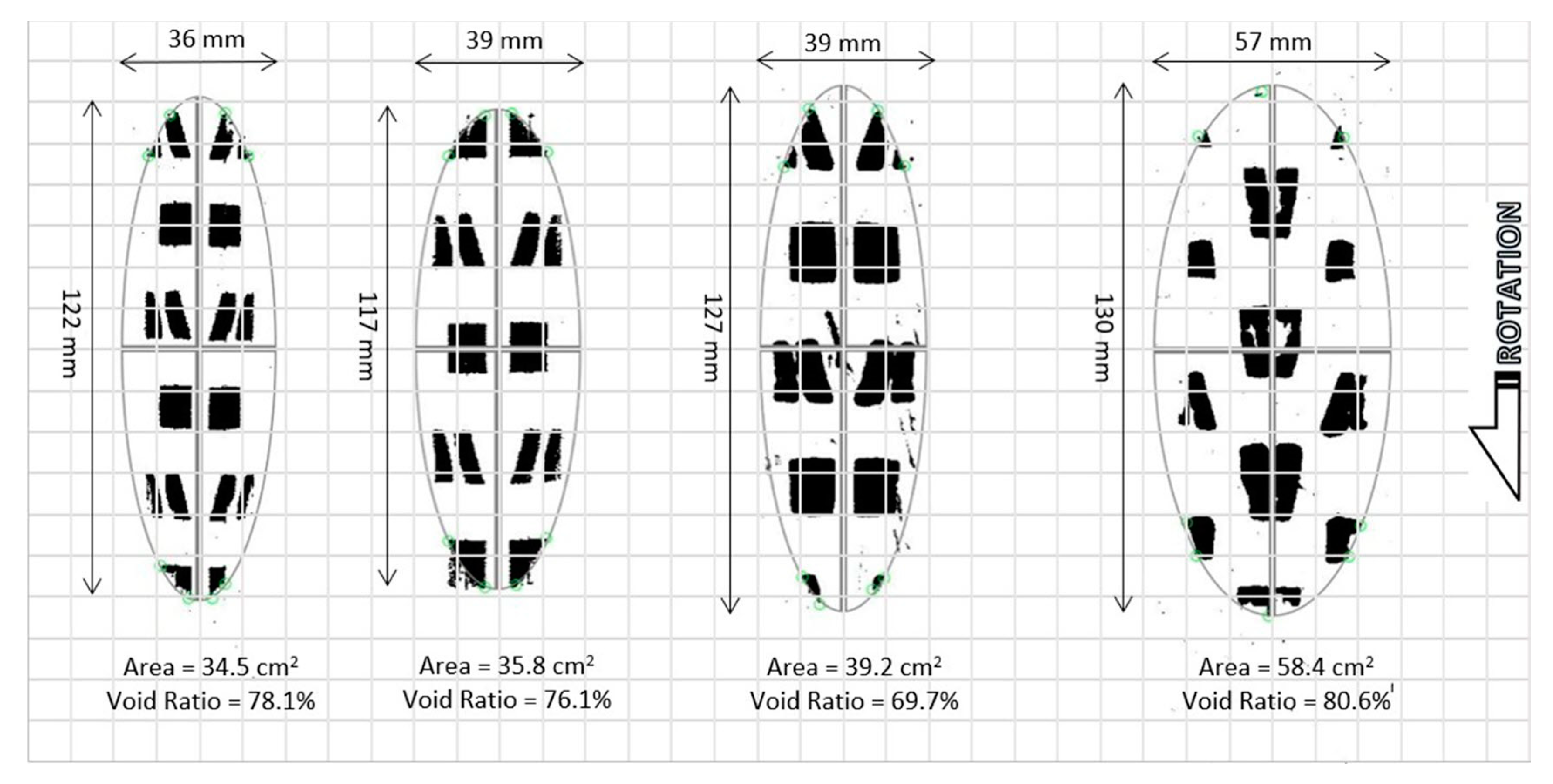
Figure 5 presents the knobby mountain bike tire footprints in the same order and on the same 10 mm grid as the cross sections in Figure 4. Here, the fitted ellipse was superimposed on the footprint and its axes were used to calculate length and width of the contact patch. Examining overall dimensions, it can be seen that the 26 × 4” fat bike tire had both the longest and widest contact patch followed in length by the 29 × 3” plus tire, the 29 × 2.3” knobby, and 27.5 × 2.8”. Hence, the length of the contact patch depended not only on tire outer diameter, but presumably also on deflection, as influenced by inflation pressure, vertical load, and the tire’s carcass. In terms of contact patch width, the 26 × 4” was widest, whereas 27.5 × 2.8” and 29 × 3” were essentially equal, despite their size designation, and the 29 × 2.3” at its nominal inflation pressure was narrower.
These images bring very clear meaning to the tire industry term “void ratio” [11]. For these knobby tires, the amount of white, empty space within the contact patch ellipse considerably exceeded the amount of black tread interacting with ground. The same MATLAB script used for fitting the ellipse also computed the void ratio by comparing white space to contact patch area after converting the image to binary. The resulting void ratios in terms of percentage for each knobby tire are listed on the figure and ranged from 69.7% to 80.6%.
As noted in the cross-sectional profiles, the tread pattern of the 27.5 × 2.8” and 29 × 3” tires essentially scaled the size and spacing of the 29 × 2.3” tread pattern upward in proportion to tire size. Again, the tread-pattern of these three tires offered no center ridge of knobs, whereas the 26 × 4” tire did.
Note that the three tread patterns on the left employed essentially two different knob typologies, one that was rectangular and one that was slightly wedge-shaped with an hourglass-shaped longitudinal groove whose depth was roughly half of the 4.5 mm tread depth. The 26 × 4” fat bike tire, on the right, showed four knob typologies within its footprint, two alternating central knob chevrons with varying degrees of central and trailing-edge relief, and two types of intermediate knobs similar to those of the other tires. Note that at zero camber angle and the inflation pressures shown, the footprints did not engage the shoulder knobs, nor the more outboard band of intermediate knobs on the 26x4” fat tire shown in the profiles of Figure 4. It should be noted that purposefully positioning the wheel’s rotation during footprint tests to engage leading and trailing knobs to better define borders of the contact patch greatly assisted in the identification of the ellipse.
Finally, these images of the footprint were useful in identifying how many knobs, pairs of knobs, or partial knobs are in contact at a given inflation pressure. This becomes relevant in a subsequent section.
3.1.3. Forces and Moments
Force and moment plots based on the Pacejka Magic coefficients and FastBike fit parameters are shown in Figure 6. Although each dataset retained a specific marker type, its line style was divided into two sections. The solid line portion, emanating from the origin, indicates values within the measurement range, whereas the dashed portion of the line represents any extrapolated values on the basis of the fit. As described previously, the limited treadmill width of the test fixture constrained slip and camber ranges, particularly for the wider knobby tires. Although the linear portion of the curve near the origin, whose slope (i.e., stiffness) was represented by the product of BCD Pacejka coefficients, was well identified, the curvature toward the peak and the eventual asymptote often had lower resolution, as was evident when comparing the 29 × 2.3” solid versus dashed line to that of the 26x4”. As such, caution should be exercised if attempting to examine peak or curvature behavior of the wider tire variants, especially in terms of slip angle.
Upon examining each of the plots in Figure 6, several interesting trends were evident. In Figure 6a, the upper left plot of normalized lateral force versus sideslip, the 29 × 2.3” had the lowest cornering stiffness. The 27.5 × 2.8”and 29 × 3” plus tires shared similar, steeper slopes but differed in curvature, whereas the 26 × 4” fat bike tire had nearly double the cornering stiffness of the baseline tire. The vertical axis was limited at a normalized force of 1.0 to highlight another interesting trend. Although the peak of the curve, whose magnitude was captured by the Pacejka D coefficient, should represent the peak frictional value (approaching 1.3 here), the tires were tested on a non-skid tape (a particular formulation of sandpaper)-coated treadmill, not on actual asphalt or dirt, which would have a commensurately lower coefficient of friction. Hence, as with most test bench characterization data, it is useful for relative comparison, while various scaling methods can be employed to adjust to an appropriate friction level if desired.
In addition to the four knobby tire curves, whose camber stiffnesses also increased with width (Figure 6b), the upper right plot of normalized lateral force due to camber also included a reference line representing the so-called tangent rule, at which point the net ground reaction force, without slip, is in the plane of the wheel [7], as shown by
where is the lateral force, N the normal load on the tire, and the camber angle.
Any tire below this line, such as the 29 × 2.3” knobby, must make up the difference via a positive sideslip angle (into the turn). The other three tires would need negative sideslip angles (slipping to the outside of the turn) for equilibrium. Depending on the tire pairing, front versus rear, this may influence the vehicle’s understeer/oversteer ratio.
The lower left plot (Figure 6c) shows the normalized self-aligning moment, which acts to align the wheel with its velocity vector, that is, diminish the tire’s slip angle. In various physical tire models, this torque can be thought of as the product of the lateral force and pneumatic trail, where the pneumatic trail is the result of an offset in the shear stress distribution toward the rear of the contact patch. An approximation of the tire pneumatic trail is shown in Figure 7, obtained by dividing the aligning moment by the lateral force due to slip, and ignoring the point at zero slip for which no lateral force exists. The shape of the pneumatic trail curve is sometimes fit with a cosine function in some versions of Pacejka’s Magic Formula. As can been seen, the tire with the longest contact patch, in this case the 26 × 4”, does not necessarily have the largest value of pneumatic trail near zero-slip, however, the other tires did follow that trend. It is possible that impending curvature of the 26 × 4” self-aligning moment was not captured due the limited slip angle measurement range for that tire. In this case, the tires with a wider contact patch with respect to their length had a pneumatic trail that decayed more slowly.
The lower right plot in Figure 6d shows normalized tire twisting torque versus camber. This torque was due to fore aft shear stress distribution across the contact patch width driven by the toroidal tire shape and acted to steer the wheel into the corner in the direction of lean. Here, the 26 × 4” fat bike tire still dominated, followed by the 27.5 × 2.8” plus tire, whereas at low camber angles the 29 × 2.3” tire trumped the 29 × 3”. It is interesting to note that at higher camber angles (or lower inflation pressures, shown later), the 29 × 3” plus tire’s twisting torque increased to a level just beyond that of the 27.5 × 2.8”. It was hypothesized that as the wider-spaced shoulder knobs of the 29 × 3” tire encounter ground, they effectively increase the width of the patch thus augmenting the twisting torque. The high twisting torque of the 26 × 4” fat bike tires seemed to corroborate the anecdotal depictions of heavy feeling, “autosteer” on many fat bikes as they were leaned into a corner, which requires the rider to counteract an increase in steering angle with significant steering effort.
3.1.4. Static Lateral and Radial Stiffness
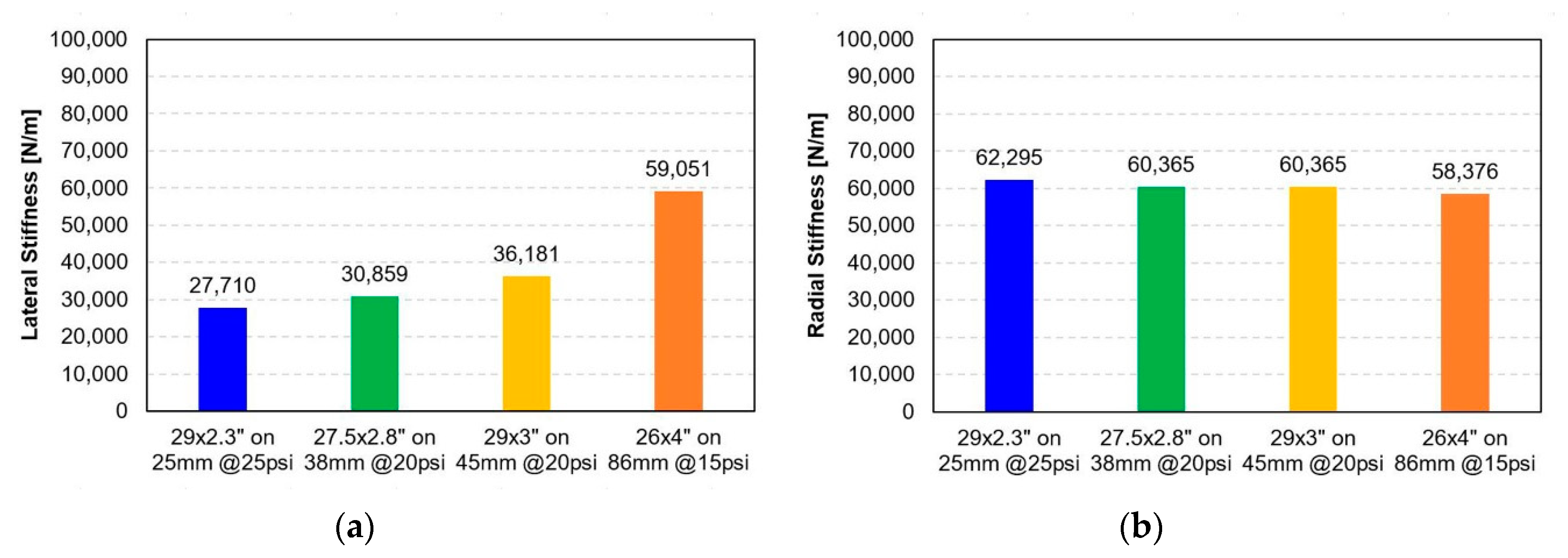
Although the static lateral and radial stiffness test was fairly straightforward and did not take into account any stiffening of the carcass due to centrifugal effects of the tire mass being accelerated radially as the wheel spins, these are still very useful parameters for understanding and modelling bicycle out of plane stability, in the case of lateral stiffness, and in-plane compliance, in the case of radial stiffness. Here, it seemed that for the given rim width and “nominal” inflation pressure selected for each size, the lateral stiffness, shown in Figure 8a, increased with tire (and/or rim) width and the radial stiffness, shown in Figure 8b for all four configurations, happened to converge around 60,000 N/m. The maximum value of the vertical axis on these plots was set to roughly the lower bound of stiffnesses for motorcycle tires [7]. Hence, bicycle tires at the inflation pressures shown were significantly less stiff than motorcycle tires.
3.2. Effect of Tread Knobs
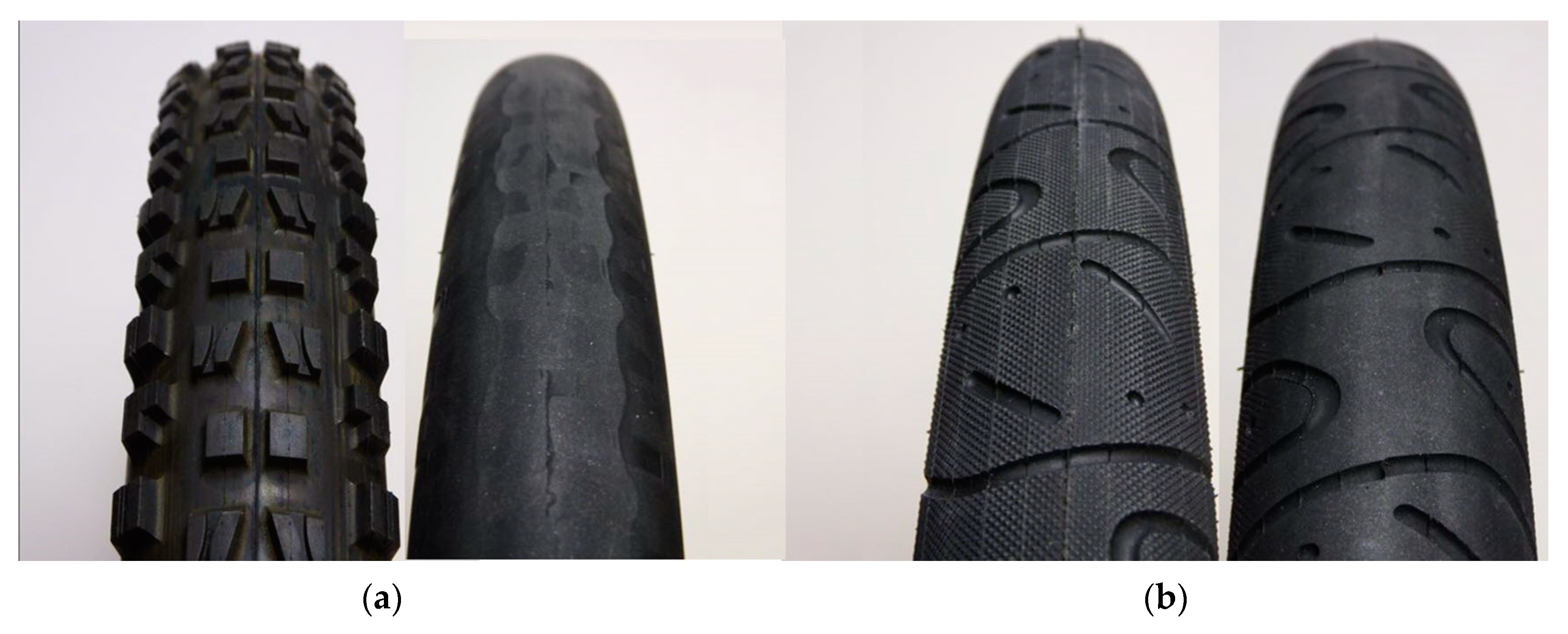
In order to examine the effect of tread knobs, this study investigated two levels of resolution. First, a less treaded tire with similar cross-sectional profile and undeformed, inflated outer radius was measured for comparison to the 29 × 2.3” knobby tire. Although this tire appeared much smoother than the knobby, it did indeed possess a “file-tread” pattern consisting of many small, pyramidal, and closely spaced knobs (each roughly 1.5 mm wide at their base and equally tall at their peak). The lesser knob height required a slightly larger tire size of 29 × 2.5” to achieve a similar outer diameter, as evident in the tire cross-sectional profiles.
After characterization of both the knobby baseline and file-tread tires, the second level of resolution involved sanding off the tread of both tires and re-characterizing what are referred to herein as the “bald” variants, as shown in Figure 9. In this case, the knobby tire became something like a true “slick” per Figure 9a, whereas the negative grooves of the file-tread in the Figure 9b tire remained. The various colors that appeared in the bald 29 × 2.3” where the knobs previously existed suggested different compounds used to form the carcass and the knobs. The results are presented in the same format as the previous section.
3.2.1. Cross-Sectional Profiles
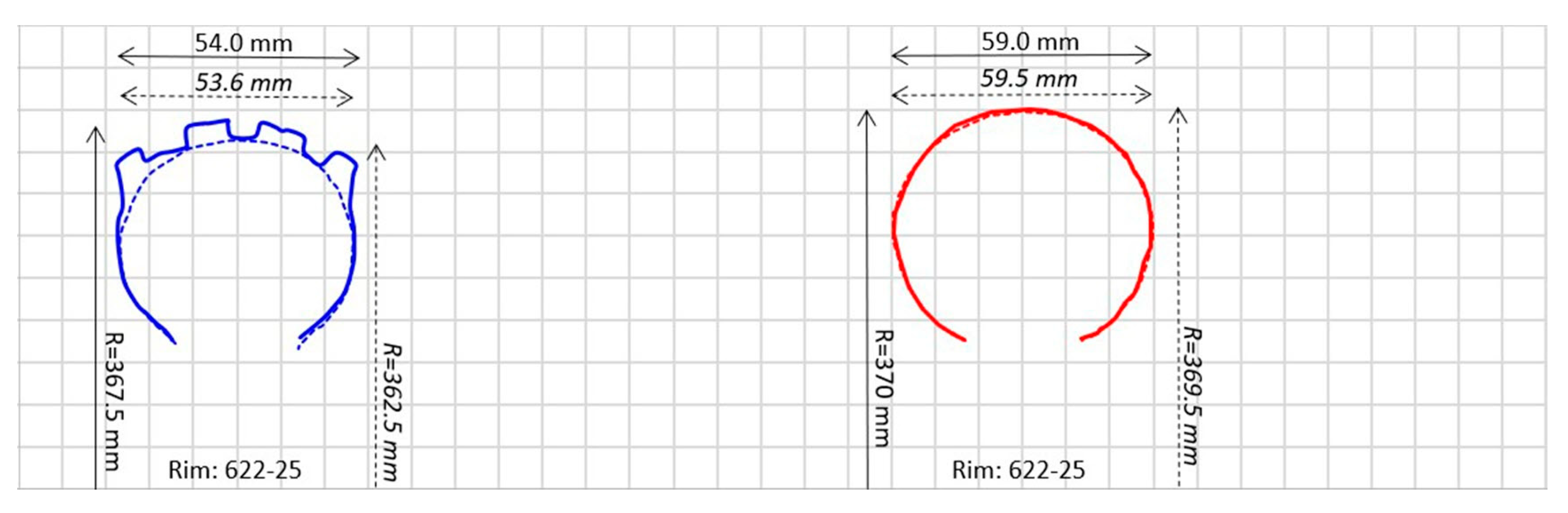
Figure 10 again shows the cross-sectional profile of the baseline 29 × 2.3” knobby tire, this time with the 29 × 2.3” “bald” variant overlaid. As captured by the measurement, all tread knobs were completely removed, and this was done around the tire’s entire circumference. Similarly, the 29 × 2.5” file-tread and 29 × 2.5” bald tire are shown in the overlay. Here, the removal of the more tightly spaced and shorter height knobs resulted in a more subtle, annular reduction in the treaded portion of the tire cross section.
3.2.2. Footprints
Figure 11 shows tire footprints for the 29 × 2.3” baseline knobby tire and bald variant, as well as the 29 × 2.5” file-tread and bald variant, all on 25 mm width rims at 25 psi (1.7 bar). The small, closely spaced file-tread knobs, as well as the negative tread grooves on the 29 × 2.5”, can be seen. The file-tread was effectively removed from the 29 × 2.5” bald variant, but the negative grooves remained. The 29 × 2.3” bald tire was essentially a slick.
The 29 × 2.3” bald contact patch was both shorter and narrower than that of the 29 × 2.3” knobby tire, whereas the 29 × 2.5” bald contact patch was longer but narrower than that of the 29 × 2.5” file-tread tire. It is interesting to note that, despite having a smaller outer radius than the 29 × 2.5” tires, the 29 × 2.3” knobby tire yielded the widest and longest contact patch of these four variants.
The relatively high (66.4%) void ratio of the 29 × 2.5” file-tread might seem surprising, as this tire was chosen as a less-treaded comparison to the 29 × 2.3” knobby (78.1%). Even after removing the file-tread pattern, the remaining negative tread grooves yielded an appreciable (19.6%) void ratio for the 29 × 2.5” bald tire, as opposed to the nearly slick (2.2%) void ratio of its 29 × 2.3” bald counterpart.
3.2.3. Forces and Moments
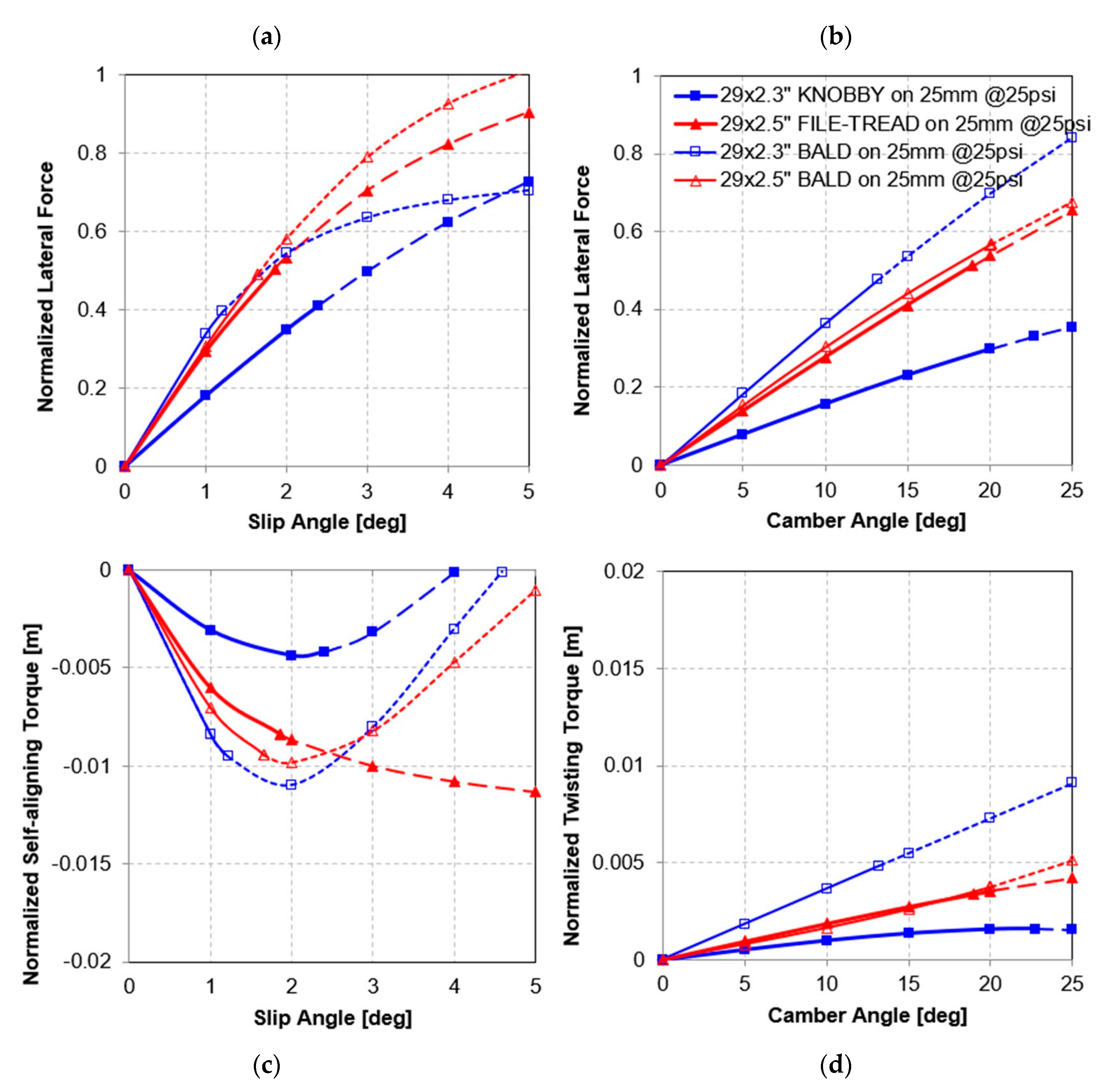
Various trends are evident in the fitted force and moment plots depicted in Figure 12. The upper left plot of normalized lateral force versus sideslip (Figure 12a) shows an increase in cornering stiffness as the tires became less treaded. There was a large increase in slope from the 29 × 2.3” knobby to the 29 × 2.3” bald tire, whereas the 29 × 2.5” file-tread to bald modification showed an increase but of less magnitude.
The same pattern was repeated in the other three plots. Removing the knobs had a big effect and removing the file-tread had a small effect, both trending in similar directions. Overall, the slick tire was the stiffest, and the knobby tire was the least stiff. As noted previously, the shape of the curve beyond the recorded data, indicated by the dashed lines, was an extrapolation based on the fit coefficients. Thus, the curvature of some of the more limited datasets may have been exaggerated.
3.2.4. Static Lateral Stiffness
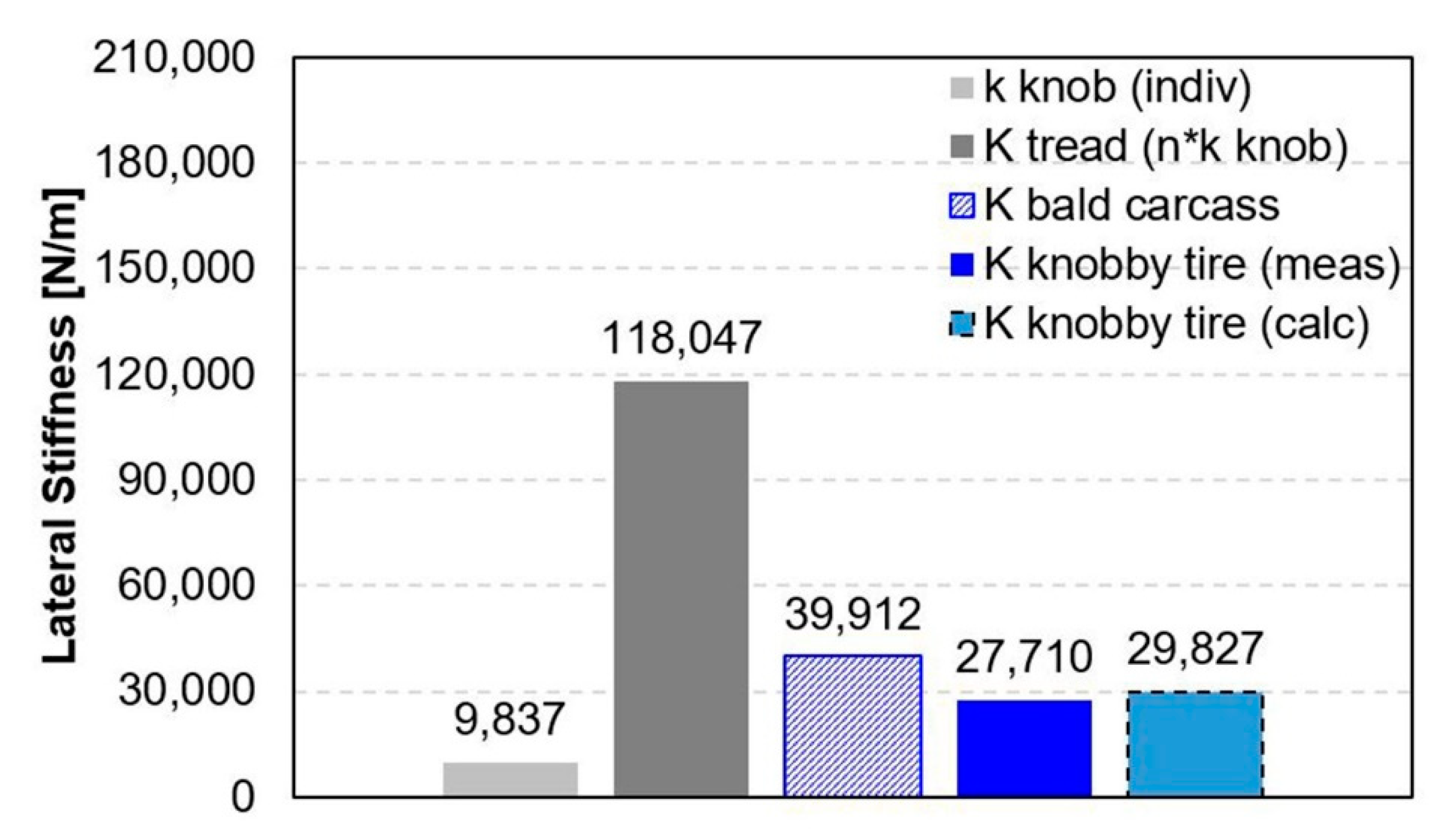
To understand the contribution of tire tread knobs to total (treaded) tire lateral stiffness, knob shear stiffness, and bald carcass lateral stiffness were measured separately and then combined, in the manner of springs in series, as in Equation (7), to compare against the measured lateral stiffness of the knobby tire.
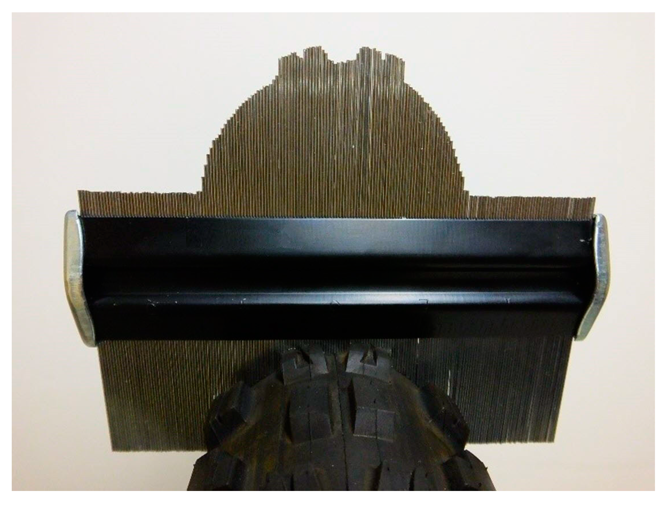
As illustrated in Figure 13, the shear stiffness of the tread knobs was measured by isolating an integral number of knobs (six shown) of an unmounted tire between matching aluminum plates. Vertical load was applied directly from the bare rim to the top aluminum plate. Then, the rim was pulled laterally while two cap screw heads prevented it from sliding relative to the upper plate. The applied lateral force and resulting lateral deflection of the rim were recorded simultaneously. The measured tread lateral stiffness was then divided by the number of knobs present between the plates to yield an approximate individual knob stiffness.
Finally, per Equation (8), the tread shear stiffness was calculated as springs in parallel by multiplying the individual knob stiffness by the number of knobs evident in the tire’s footprint.
These respective stiffness values and the comparison of measured versus calculated total tire stiffness are shown for the 29 × 2.3” knobby tire in Figure 14.
As can be seen, the approximate total tire stiffness matched well (within 8%) with the measured lateral stiffness of the inflated knobby tire. Possible sources of variation included difficulty in determining exactly how many knobs, or fractions thereof, were included in the contact patch. This approach also assumed equal stiffness contribution from various knob typologies and ignored possible variation in load distribution across the patch. A similar investigation was not repeated for the file-tread pattern because of the impracticality of counting and measuring the stiffness of an integral number of the file-tread knobs.
3.3. Effect of Inflation Pressures and Rim Width
Tire inflation pressure is an important setup and tuning parameter for mountain bike applications. A happy compromise between traction, durability, protection for the rim, handling, and ride characteristics often depends on rider weight, bike fitment, terrain, even surface, or soil consistency, and of course, rider preference. Potentially for this reason, bicycle manufacturers, unlike automotive or motorcycle companies, rarely specify a specific recommended operating inflation pressure for each vehicle model and leave it to the end-user to experiment within the bounds typically designated on the tire sidewall. Thus, to better explore the potential operating range of various tires mentioned thus far in this study, additional measurements were taken at various inflation pressures. These results are reported in a format much like the previous sections.
3.3.1. Footprints
Figure 15 and Figure 16 illustrate the effect of varying inflation pressure on the tire footprints for the 29 × 2.3” knobby tire on 25 mm rim. The images show that as inflation pressure increased from left to right, the contact patch length and width became smaller and thus contact patch area was reduced. Interestingly, for the 29 × 2.3” knobby tire at 10 psi, in the leftmost plot, the tire deformed enough for the shoulder knobs to contact the ground (even at zero camber), and thus the shape of the patch became significantly wider. As inflation pressure increased, fewer and fewer individual knobs remained in the contact patch.
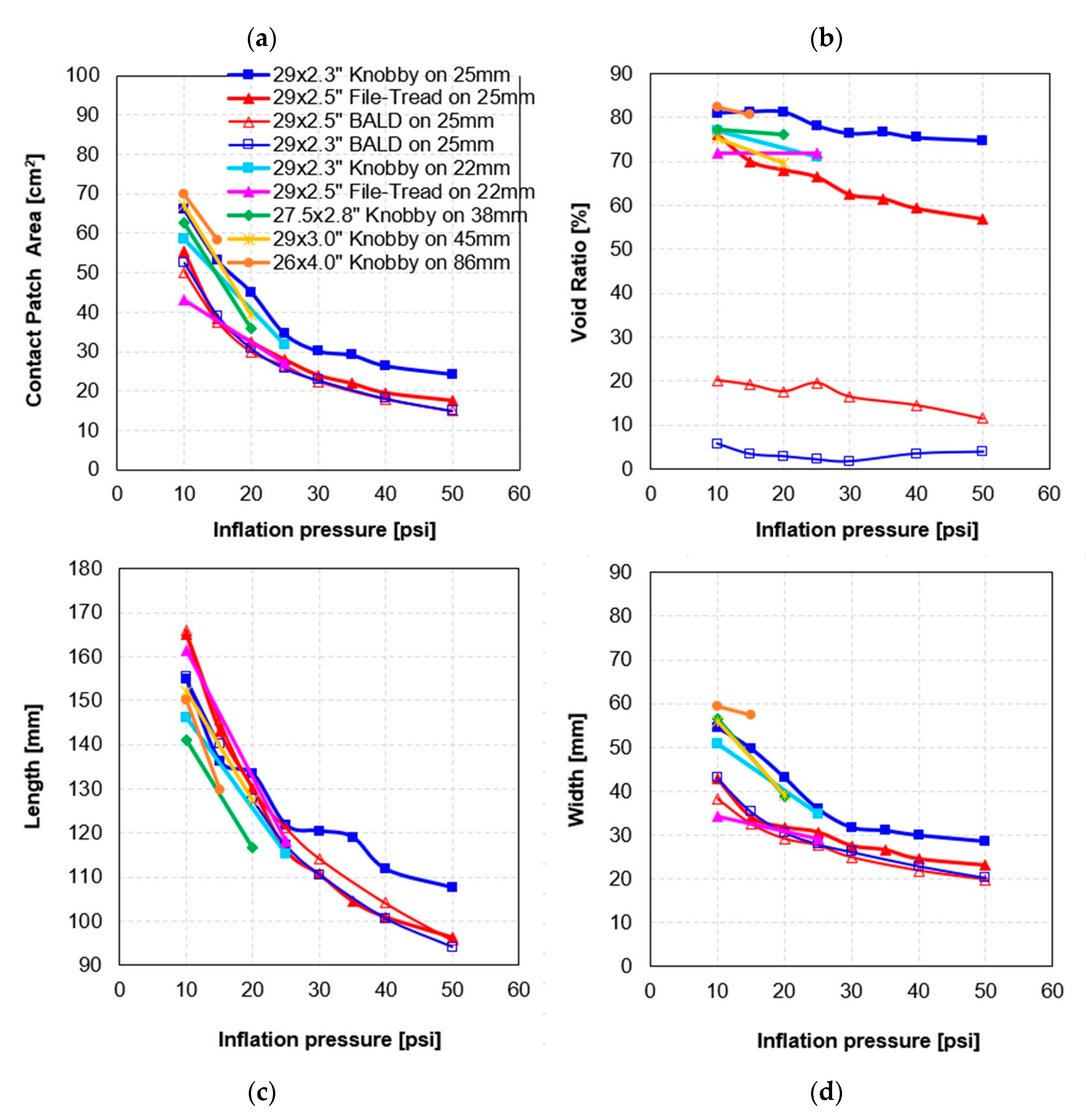
Figure 16 shows contact patch characteristics as functions of inflation pressure. The 29 × 2.3” knobby, 29 × 2.3” bald, 29 × 2.5” file-tread, and 29 × 2.5” bald tires were measured at eight pressure increments. This gave added resolution to various trends. The other three knobby tires in 27.5 × 2.8”, 29 × 3”, and 26 × 4” are also shown, but with inflation pressure at just two levels, 10 psi (potential use case for lightweight riders or usage on soft or loose terrain), and the “nominal” pressure considered in previous sections. Finally, two additional datapoints of the 29 × 2.3” knobby and 29 × 2.5” file-tread tire on slightly narrower, 22 mm internal rim widths are shown to begin to explore those effects.
The upper left plot (Figure 16a) suggests the ranking of tires in terms of contact patch area varied somewhat with inflation pressure, but in general the contact patch area decreased in a seemingly nonlinear fashion with increasing inflation pressure. Here, the 26x4” fat bike tire remained near the largest, whereas the 29 × 2.3” knobby surpassed the plus tires between 10 and 20 psi. The contact patch area of the less-treaded tires in the form of the 29 × 2.5” file-tread on the 25 mm rim, 29 × 2.3” bald, and 29 × 2.5” bald tire seemed slightly more sensitive in the lower pressure regime (from 10 to 15 psi), whereas as pressure was increased (beyond 20 psi), the curvature stabilized. The 29 × 2.3” knobby on 22 mm rim and 29 × 2.5” file-tread tire on 22 mm rims showed a small decrement in contact patch area with respect to their 25 mm rim variants.
The upper right plot (Figure 16b) depicts how the tread void ratio within the contact patch area varied between tires and with inflation pressure. It is quite clear that the knobby tires had higher void ratios than the 29 × 2.5” file-tread on 25 mm rim at all but the lowest inflation pressure. The 26 × 4” fat bike tire and 29 × 2.3” knobby tire were both around 80% void ratio at low pressures, which for the 29 × 2.3” knobby tire on 25 mm rim fell to 74% at 50 psi. Seemingly, scaling the knob size up for the 27.5 × 2.8” and 29 × 3” plus tires caused a small reduction in their void ratio with respect to the 29 × 2.3” knobby tire on the 25 mm rim. The void ratio of the 29 × 2.5” bald tire, which contained only the negative grooves, reduced from 20% to 10% with increasing inflation pressure, whereas the nearly slick 29 × 2.3” bald tire hovered at a void ratio less than 5%.
The lower two plots show the contact patch length (Figure 16c) and width (Figure 16d) versus inflation pressure. Here, the length was generally at least twice the width or more. The change in lengths of most of the tires shown were similar, whereas the 26 × 4” fat and 27.5 × 2.8” plus tires were slightly shorter than others at the same inflation pressures. The 29 × 2.3” knobby tire retained a slightly longer contact patch than the 29 × 2.5” file-tread tire or their bald counterparts at inflation pressures above 25 psi (1.7 bar). Finally, in terms of width, there was a clear grouping between the wider contact patch of the knobby tires and the less-wide patch of the file-tread and bald variants.
3.3.2. Forces and Moments
Figure 17 shows the stiffness coefficients for slip and camber forces as well as self-aligning and twisting torques versus inflation pressure.
The upper left plot (Figure 17a) displays various trends in cornering stiffness coefficient. First, large differences were apparent between the different tire sizes bounded on the upper end by the 26 × 4” fat bike and 29 × 2.3” bald tires, with upper values in excess of 20 1/rad, and on the lower end by the 29 × 2.3” knobby tire, on either rim width, at around 10 1/rad. Aside from the 26 × 4” fat tire, the less-treaded tires had higher cornering stiffness above 20 psi (1.4 bar). Additionally, above this pressure, the cornering stiffness of the tires shown seemed to vary little with further increase in inflation pressure. Below this pressure, there were some nonlinear and disparate behaviors where cornering stiffness of the 29 × 2.5” file-tread increased rapidly with inflation pressure whereas that of the 29 × 2.3” knobby tire decreased gradually. Across the limited pressures measured, the 27.5 × 2.8” plus tire exhibited a different sensitivity (slope) than the other knobby tires.
The plot of normalized camber stiffness, shown in the upper right (Figure 17b) showed similar overall groupings. The less-treaded variants exhibited higher camber stiffness coefficients, with a decreasing trend as inflation pressure increased, and the 29 × 2.3” bald tire topped the chart. Camber stiffness of the knobby tires fell off more quickly from 10 to 25 psi, whereas the 29 × 2.3” knobby tire on a 25 mm rim eventually achieved a slope similar to its less-treaded counterparts, albeit at a lower value (below 1.0 1/rad). Rim width had minimal effect.
In the lower left plot (Figure 17c), the sign convention for the aligning torque should be kept in mind. Its value was negative because it acted to reduce the tire slip angle, and thus a larger stiffness magnitude resulted in a more negative value. Again, there was a grouping. Except for the 26 × 4” fat bike tire at 10 psi, the less treaded tires exhibited more self-aligning stiffness, with increased inflation pressure, albeit with diminishing magnitude. The 29 × 2.3” and 27.5 × 2.8” knobby tires grouped fairly close together with the lowest magnitudes of self-aligning stiffness. It should be noted that although the units of normalized self-aligning stiffness were in meters, this value was different from the pneumatic trail. As described earlier, the pneumatic trail can be derived by dividing the tire self-aligning moment by the lateral force due to slip (at zero camber).
Normalized twisting torque stiffness, shown in the lower right plot (Figure 17d), showed a fairly rapid decrease with increasing inflation pressure up to about 30 psi (2.1 bar) for the measured tires. On the basis of the higher twisting torque stiffness magnitudes of the 29 × 2.3” bald and 26 × 4” tires, one would expect them to generate the most steering torque at low inflation pressures. For the 26 × 4”, this was likely related to the difference in peripheral velocity across such a wide patch, and for the 29 × 2.3” bald tire it may have been related to the relatively small toroid radius and steep shoulder drop. Again, a minor change in rim width had minimal effect. Presumably, the steep slope of the 27.5 × 2.8” and 29 × 3” plus tires between 10 and 15 psi may have been related to the widely spaced shoulder knobs contacting at lower lean angles on the less inflated, softer, and more deformed tire.
3.3.3. Static Lateral Stiffness
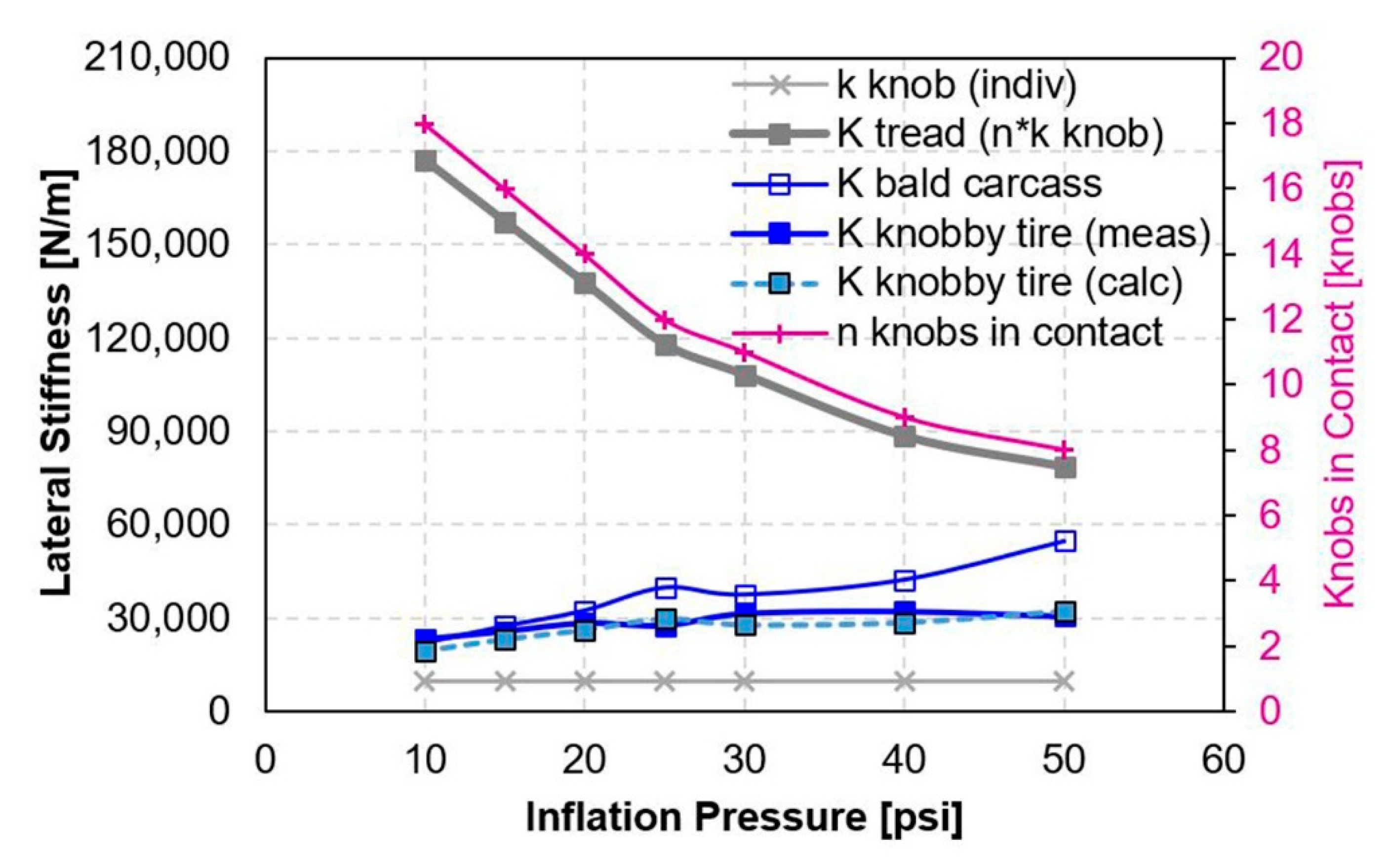
Section 3.2.4 described modelling the tire static lateral stiffness as multiple individual knobs acting as springs in parallel that constituted the tread stiffness. The tread stiffness then combined with the bald carcass stiffness as springs in a series to yield the total lateral stiffness of the treaded tire. Now, in Figure 18, that simplified model is applied across a range of inflation pressures, yielding results comparable to the measured value of the 29 × 2.3” knobby tire. The figure shows the individual knob stiffness as derived from the tread shear measurement multiplied by the number of knobs in contact. On the basis of the footprints shown in Figure 15, “n”, the number of knobs in contact, plotted here on the secondary axis, decreased with inflation pressure. Hence, the product of those terms yielded the theoretical tread stiffness, which also decreased with inflation pressure. It is interesting to note that the individual knobs did not change in stiffness, but the fact that fewer of them were in contact reduced the effective tread stiffness. Meanwhile, the as-measured bald carcass stiffness was shown to increase with inflation pressure. Combining these two as springs in series resulted in a theoretical total tire lateral stiffness within 15% of the measured values across the range of inflation pressures.
As before, possible sources of the difference between calculated and measured total stiffness included difficulty in determining exactly how many knobs, or fractions thereof, were included in the contact patch and, for low inflation pressures, the participation of shoulder knobs, whose shear stiffness was not measured.
4. Conclusions
Characterization of four modern mountain bike tire sizes was carried out on appropriate rim widths at what were considered realistic nominal inflation pressures. Tire cross sections were compared, and tire radii and width values reported. Tire footprints at zero camber angle and realistic normal load were fit as ellipses and their area, geometry, void ratios, and tread patterns were discussed. Force and moment measurements were conducted using the measuring device at the University of Wisconsin–Milwaukee. A combination of Pacejka’s Motorcycle Magic Tire Model and FastBike twisting torque polynomial were fitted to the data to yield parametric tire model coefficients. These fitted curves were then used to compare lateral force due to slip and camber, as well as self-aligning moment and twisting torque. Good resolution of the linear portion of the respective stiffness curves were obtained, whereas tire versus treadmill width limited identification of curvature and peak friction values to some extent. Static lateral and radial carcass stiffnesses were shown. The compilation of these results suggests appreciable differences in tire performance among 29 × 2.3”, 27.5 × 2.8”, 29 × 3”, and 26 × 4” knobby tires.
Additional characterization was carried out to quantify the effects of tire tread knobs. A 29 × 2.3” knobby tire was compared to a file-tread tire of similar size. The treads were then removed from both tires, and characterization of the resultant bald tires further informed this comparison. It was shown that file-tread and a tread pattern with negative grooves had appreciable void ratios and performance trade-offs that were different from a truly bald, slick tire. It was also shown that for the 29 × 2.3” knobby mountain bike tire studied, the combination of tire tread shear stiffness, obtained by combining individual knobs as springs in parallel, with the inflated bald tire carcass as springs in series, yielded a lateral stiffness value similar to that measured for the total treaded tire.
Finally, the aforementioned footprint, force and moment, and static carcass lateral stiffness parameters for each tire were compared across a range of inflation pressures. Results suggest some differences between knobby and less-treaded tires, especially at higher inflation pressures. Inflation pressure influenced the number of knobs interacting with ground as the toroidal tires deformed. Incorporating this observation into the approximation of tire lateral stiffness as a combination of tread shear stiffness and carcass lateral stiffness as springs in series seemed promising. A brief comparison of a 25 mm and 22 mm rim suggested small relative differences for the two tires measured.
Ideally, this work supplements ongoing progress in bicycle modelling and simulation [12]. Parametrization of nonlinear tire properties, as shown here, may aide higher fidelity bicycle and even mountain bike handling and stability simulations. A further study looking at alternate tire sizes, specifications, and tread patterns; isolating individual knob typologies; and implementing a wider treadmill would be interesting. Applying similarity methods to link tire performance to width and radius may warrant additional study, whereas a design of experiments (DOE) approach focused on the effects of specific construction parameters would benefit from bicycle tire manufacturer support in building relevant test samples.
Author Contributions
Conceptualization, J.S. and A.D.; methodology, A.D.; software, A.D. and J.S.; validation, A.D. and J.S.; formal analysis, J.S. and A.D.; investigation, A.D. and J.S.; resources, A.D.; data curation, A.D. and J.S.; writing—original draft preparation, J.S. and A.D.; writing—review and editing, A.D. and J.S.; visualization, J.S.; supervision, J.S.; project administration, A.D.; funding acquisition, J.S. All authors have read and agreed to the published version of the manuscript.
Funding
This research received no external funding.
Conflicts of Interest
The authors declare no conflict of interest.
References
- Statista: Number of Participants in Mountain/Non-Paved Surface Bicycling in the United States from 2011 to 2018 (in Millions). Available online: https://www.statista.com/statistics/763737/mountain-non-paved-surface-bicycling-participants-us/ (accessed on 3 April 2019).
- Statista: Bicycle Sales in the United States by Category of Bike in 2017. Available online: https://www.statista.com/statistics/236150/us-retail-sales-of-bicycles-and-supplies/J.Y. (accessed on 3 April 2019).
- Dressel, A. Measuring and Modeling the Mechanical Properties of Bicycle Tires. Ph.D. Thesis, The University of Wisconsin-Milwaukee, Milwaukee, WI, USA, 2013. [Google Scholar]
- Pacejka, H.B. Tyre and Vehicle Dynamics, 2nd ed.; Butterworth and Heinemann: Oxford, UK, 2006. [Google Scholar]
- FastBike 6.3.1 User Manual; Dynamotion: Padova, Italy, 2006; p. 36.
- Doria, A.; Tognazzo, M.; Cusimano, G.; Bulsink, V.; Cooke, A.; Koopman, B. Identification of the mechanical properties of bicycle tyres for modelling of bicycle dynamics. Veh. Syst. Dyn. 2013, 51, 405–420. [Google Scholar] [CrossRef]
- Cossalter, V. Motorcycle Dynamics, 2nd ed.; Lulu Press: Morrisville, NC, USA, 2006. [Google Scholar]
- Gent, A.; Walter, J. The Pneumatic Tire; NHTSA: Washington, DC, USA, 2006. [Google Scholar]
- Cossalter, V.; Doria, A. The relation between contact path geometry and the mechanical properties of motorcycle tires. Veh. Syst. Dyn. 2005, 43, 156–167. [Google Scholar] [CrossRef]
- Wallaschek, J.; Wies, B. Tyre tread-block friction: Modelling, simulation and experimental validation. Veh. Syst. Dyn. 2013, 51, 1017–1026. [Google Scholar] [CrossRef]
- Jansen, S.; Schmeitz, A.; Akkermans, L. Study on Some Safety-Related Aspects of Tyre Use; European Commission: Brussels, Belgium, 2014. [Google Scholar]
- Klug, S.; Moia, A.; Verhagen, A.; Georges, D.; Savaresi, S. Control-Oriented modeling and validation of bicycle curve dynamics with focus on lateral tire parameters. In Proceedings of the 2017 IEEE Conference on Control Technology and Applications (CCTA), Mauna Lani, HI, USA, 27–30 August 2017; pp. 86–93. [Google Scholar]
Figure 1.
Capturing mountain bike tire tread profile with carpenter’s contour gauge.

Figure 2.
Tire force and moment measuring device at the University of Wisconsin–Milwaukee.
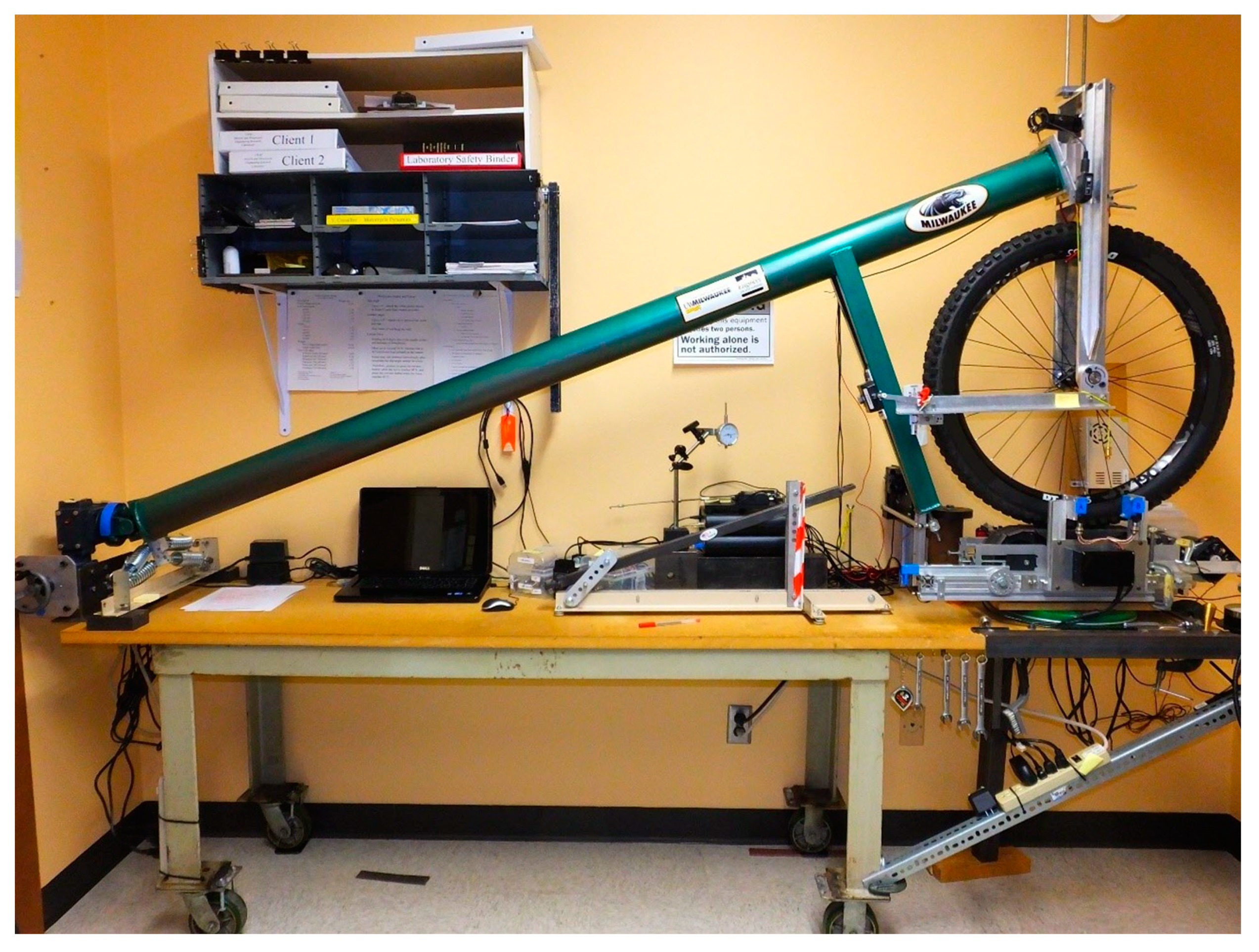
Figure 3.
Force and moment raw data, smoothed lines, and fit curves for 29 × 2.3” knobby on 25 mm rim at 25 psi (1.7 bar) with (a) normalized lateral force vs. slip angle, (b) normalized lateral force vs. camber angle, (c) normalized self-aligning moment vs. slip angle and (d) normalized twisting torque vs. camber angle.
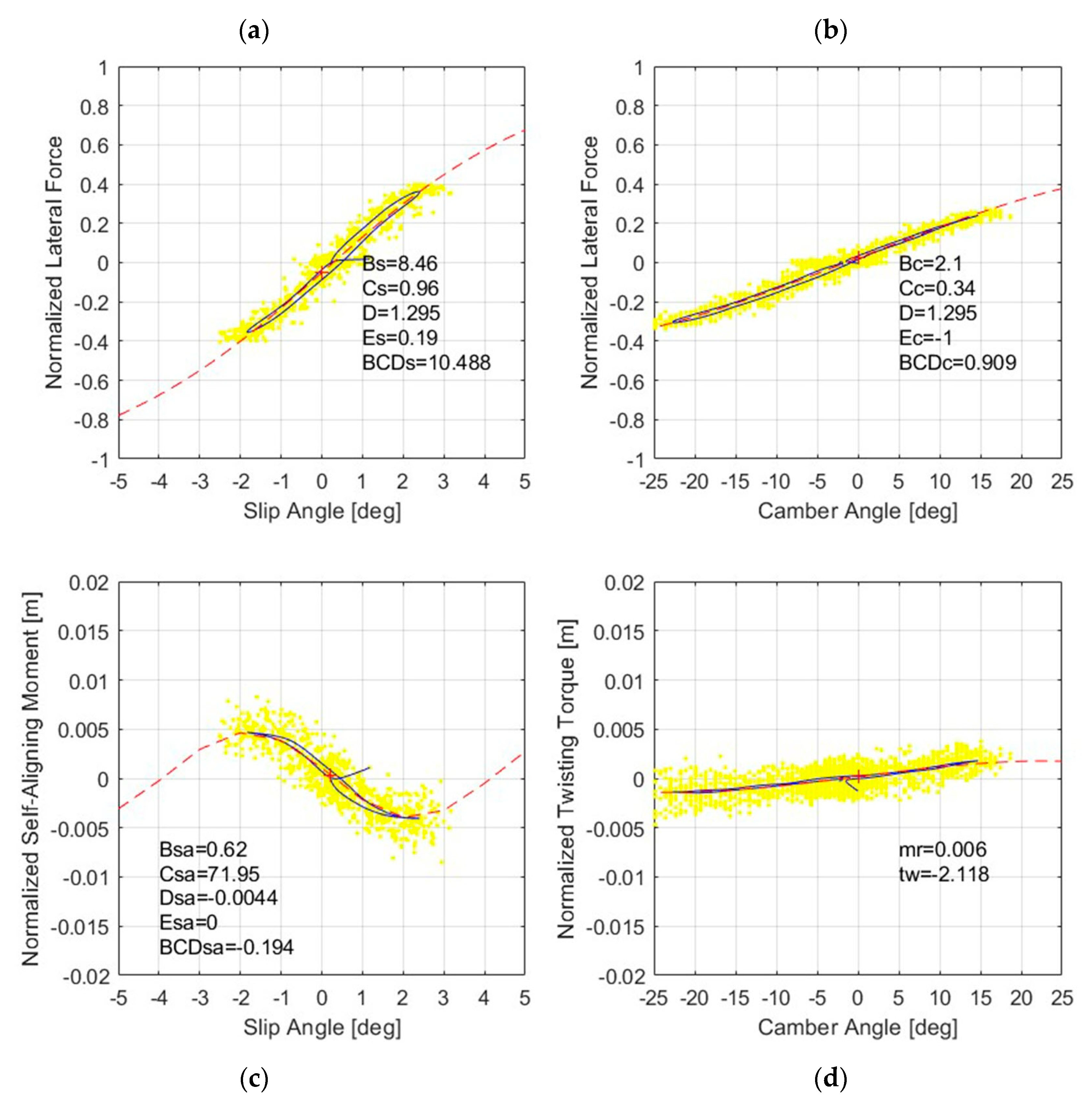
Figure 4.
Cross sectional profiles for 29 × 2.3”, 27.5 × 2.8”, 29 × 3”, and 26 × 4” knobby tires, respectively.
Figure 4.
Cross sectional profiles for 29 × 2.3”, 27.5 × 2.8”, 29 × 3”, and 26 × 4” knobby tires, respectively.
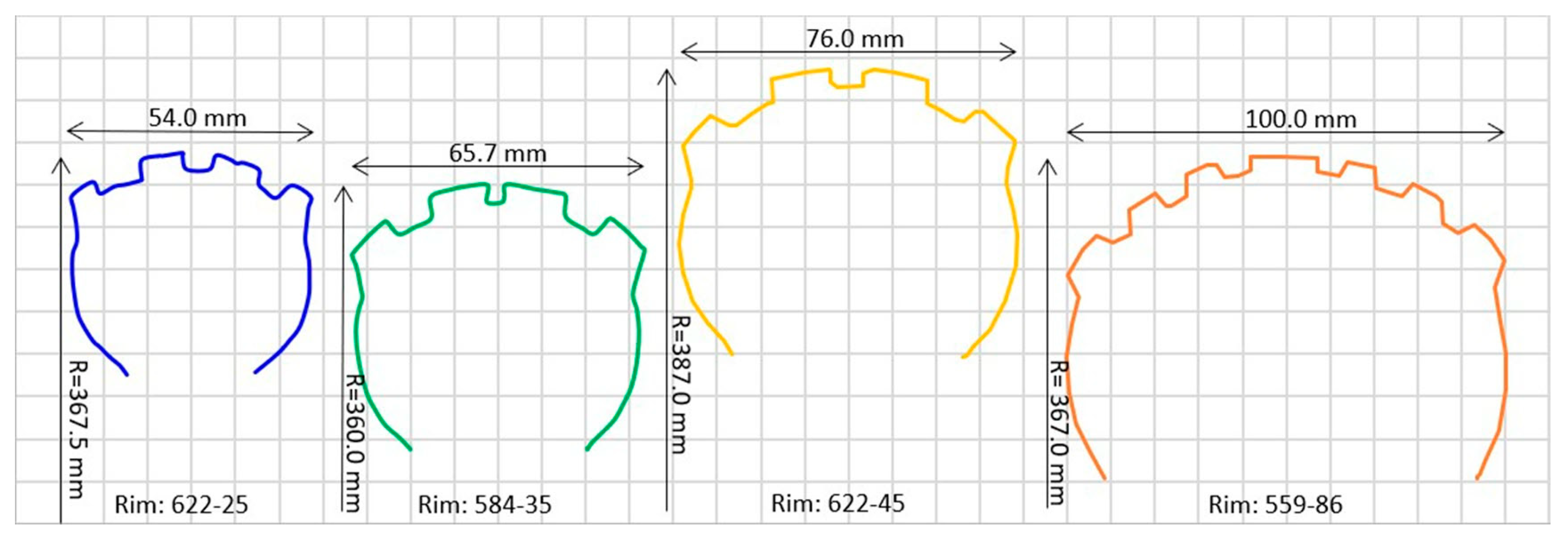
Figure 5.
Footprints for 29 × 2.3”, 27.5 × 2.8”, 29 × 3”, and 26 × 4” knobby tires, respectively.

Figure 6.
Force and moment fitted curves for 29 × 2.3”, 27.5 × 2.8”, 29 × 3”, and 26 × 4” knobby tires with (a) normalized lateral force vs. slip angle, (b) normalized lateral force vs. camber angle, (c) normalized self-aligning moment vs. slip angle and (d) normalized twisting torque vs. camber angle.
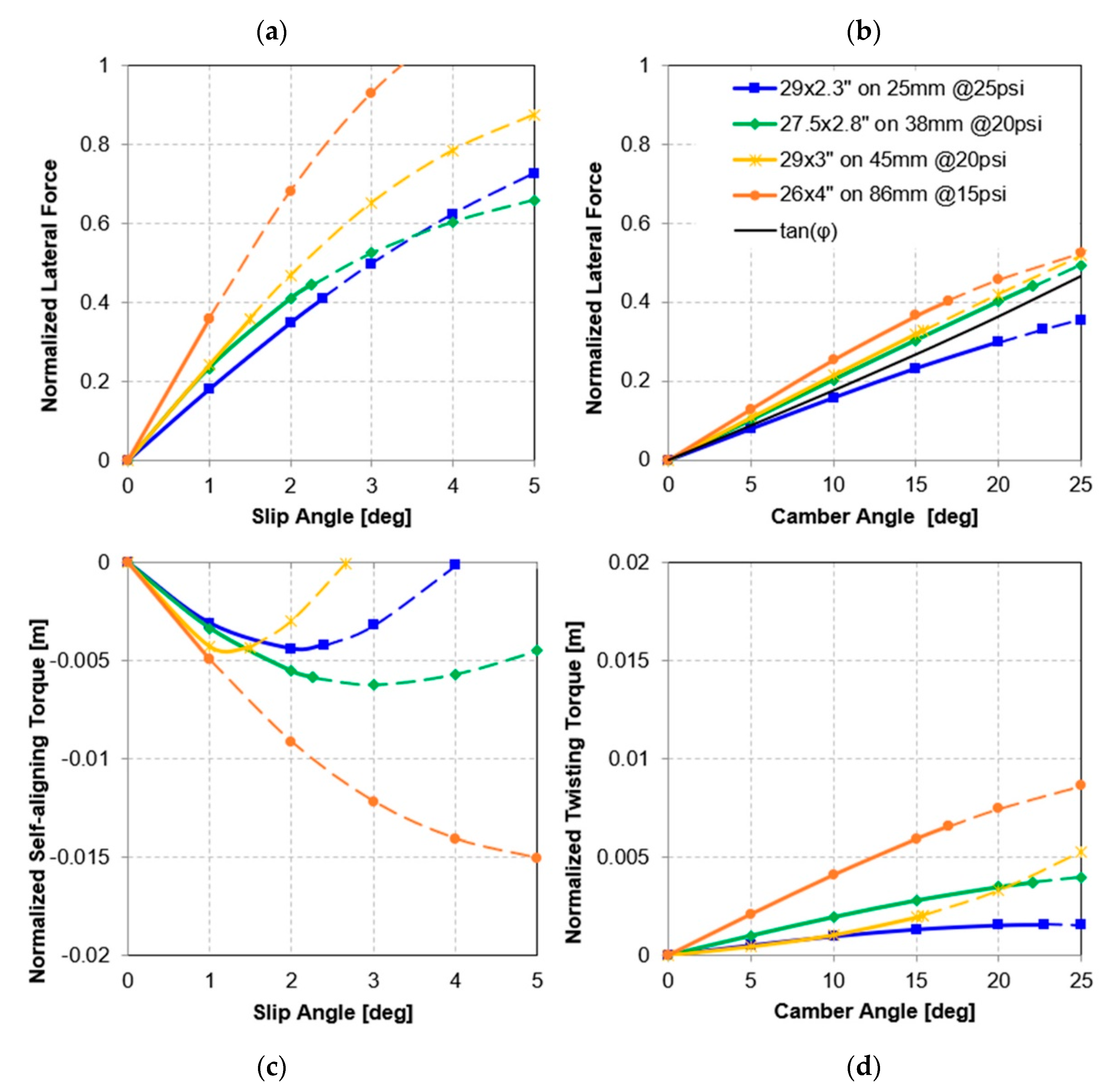
Figure 7.
Calculated pneumatic trail for 29 × 2.3”, 27.5 × 2.8”, 29 × 3”, and 26 × 4” knobby tires.
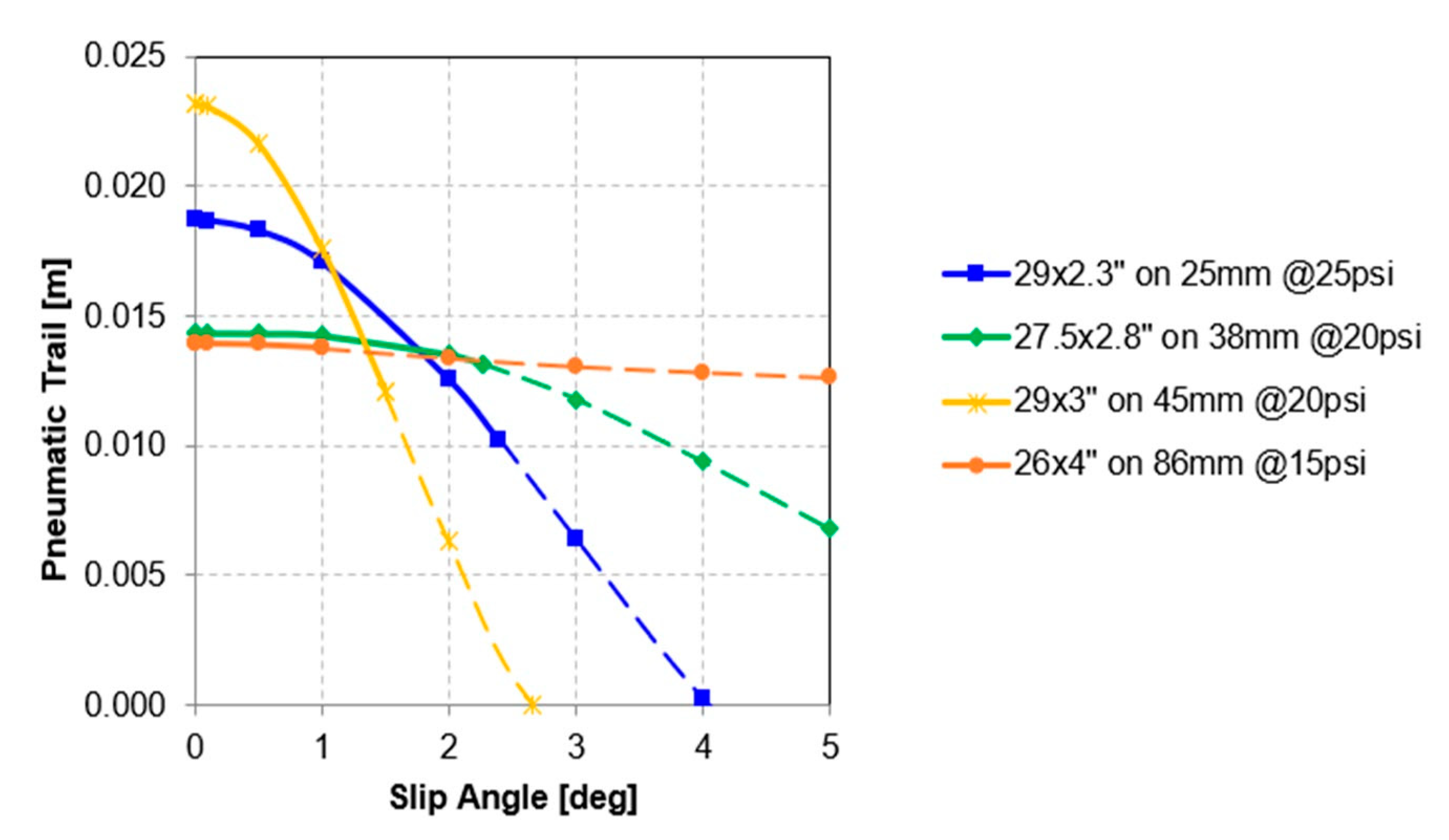
Figure 8.
(a) Static lateral and (b) radial stiffness of 29 × 2.3”, 27.5 × 2.8”, 29 × 3”, and 26 × 4” knobby bicycle tires.
Figure 8.
(a) Static lateral and (b) radial stiffness of 29 × 2.3”, 27.5 × 2.8”, 29 × 3”, and 26 × 4” knobby bicycle tires.

Figure 9.
Images of (a) original treaded 29 × 2.3” knobby and its bald tire counterpart and (b) the 29 × 2.5” file-tread tire with its bald tire counterpart.
Figure 9.
Images of (a) original treaded 29 × 2.3” knobby and its bald tire counterpart and (b) the 29 × 2.5” file-tread tire with its bald tire counterpart.

Figure 10.
Cross sectional profiles of 29 × 2.3” knobby tire (solid) overlaid with its bald variant (dashed), on the left, and 29 × 2.5” file-tread tire (solid) overlaid with its bald variant (dashed), on the right.
Figure 10.
Cross sectional profiles of 29 × 2.3” knobby tire (solid) overlaid with its bald variant (dashed), on the left, and 29 × 2.5” file-tread tire (solid) overlaid with its bald variant (dashed), on the right.

Figure 11.
Footprints for 29 × 2.3” knobby, 29 × 2.3” bald, 29 × 2.5” file-tread, and 29 × 2.5” bald tires at 25 psi (1.7 bar) on 25 mm inner width rim.
Figure 11.
Footprints for 29 × 2.3” knobby, 29 × 2.3” bald, 29 × 2.5” file-tread, and 29 × 2.5” bald tires at 25 psi (1.7 bar) on 25 mm inner width rim.
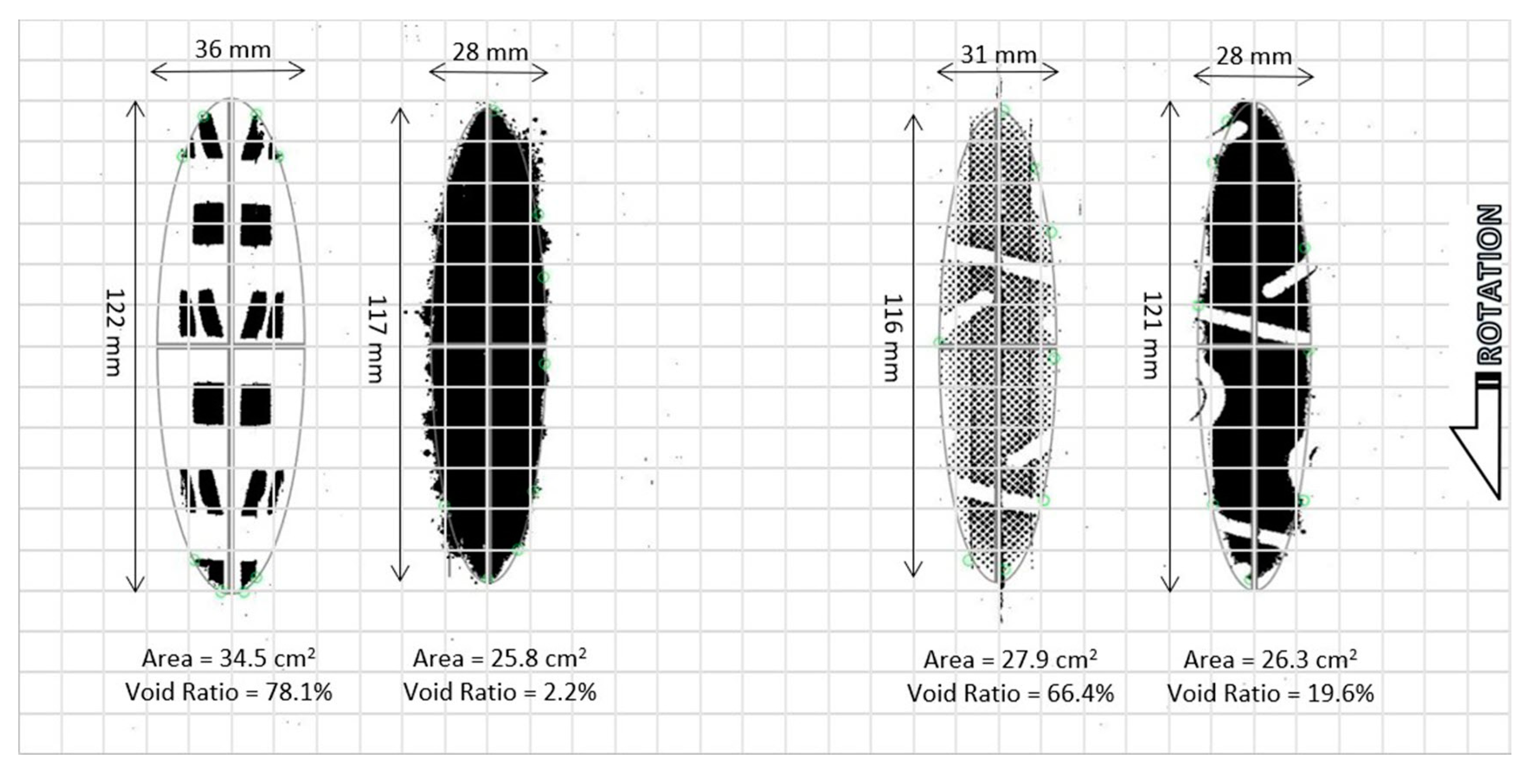
Figure 12.
Force and moment fitted curves for 29 × 2.3” knobby, 29 × 2.3” bald, 29 × 2.5” file-tread, and 29 × 2.5” bald tires at 25 psi (1.7 bar) on 25 mm inner width rim with (a) normalized lateral force vs. slip angle, (b) normalized lateral force vs. camber angle, (c) normalized self-aligning moment vs. slip angle and (d) normalized twisting torque vs. camber angle.

Figure 13.
Schematic illustrating non-destructive measurement of lateral shear stiffness of tire tread knobs via loads applied to unmounted tire squeezed between appropriately sized aluminum plates.
Figure 13.
Schematic illustrating non-destructive measurement of lateral shear stiffness of tire tread knobs via loads applied to unmounted tire squeezed between appropriately sized aluminum plates.
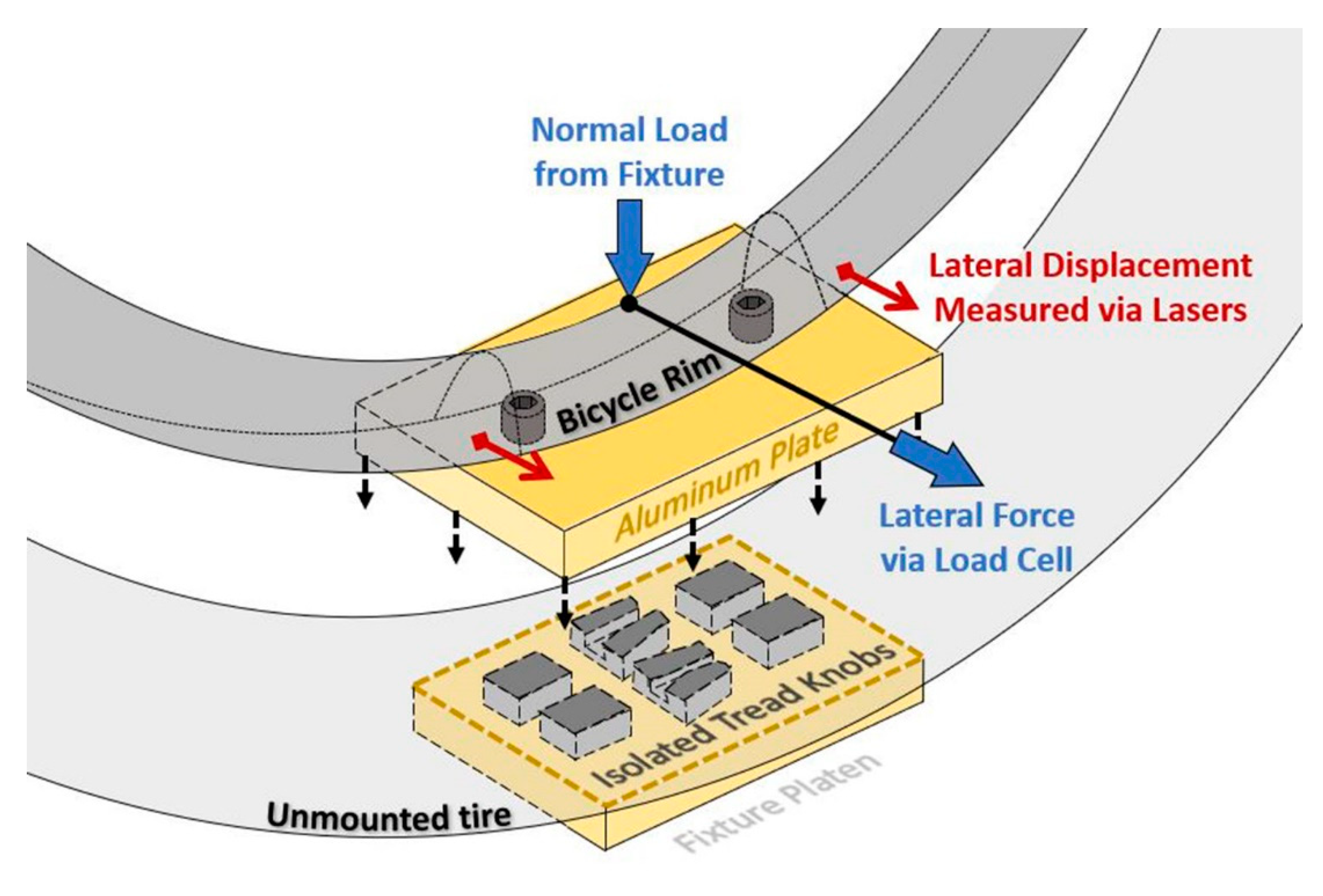
Figure 14.
Bar chart of knob, tread, bald carcass, measured, and calculated total tire stiffness for 29 × 2.3” knobby tire comparing relative stiffness magnitudes at 25 psi (1.7 bar).
Figure 14.
Bar chart of knob, tread, bald carcass, measured, and calculated total tire stiffness for 29 × 2.3” knobby tire comparing relative stiffness magnitudes at 25 psi (1.7 bar).

Figure 15.
Footprints for 29 × 2.3” knobby tire at inflation pressures of 10, 20, 30, 40, and 50 psi (0.7, 1.4, 2.1, 2.8, and 3.4 bar) from left to right on 25 mm inner width rim.
Figure 15.
Footprints for 29 × 2.3” knobby tire at inflation pressures of 10, 20, 30, 40, and 50 psi (0.7, 1.4, 2.1, 2.8, and 3.4 bar) from left to right on 25 mm inner width rim.
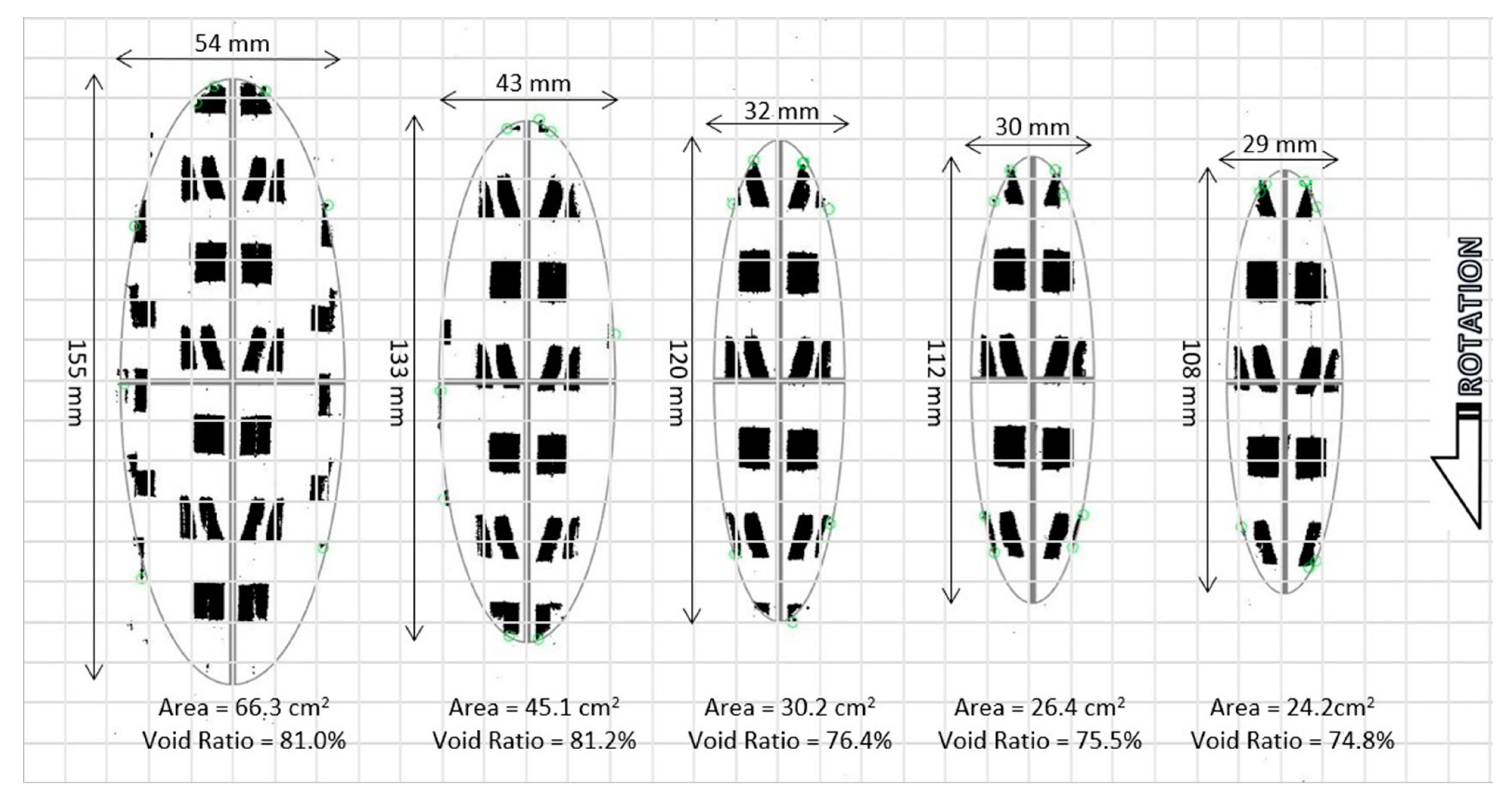
Figure 16.
Tire footprint parameters versus inflation pressure for various bicycle tires with (a) contact patch area, (b) void ratio, (c) contact patch length and (d) contact patch width.
Figure 16.
Tire footprint parameters versus inflation pressure for various bicycle tires with (a) contact patch area, (b) void ratio, (c) contact patch length and (d) contact patch width.

Figure 17.
Force and moment fitted stiffness coefficients versus inflation pressure for various bicycle tires with (a) cornering stiffness, (b) camber stiffness, (c) self-aligning stiffness and (d) twisting torque coefficients.
Figure 17.
Force and moment fitted stiffness coefficients versus inflation pressure for various bicycle tires with (a) cornering stiffness, (b) camber stiffness, (c) self-aligning stiffness and (d) twisting torque coefficients.
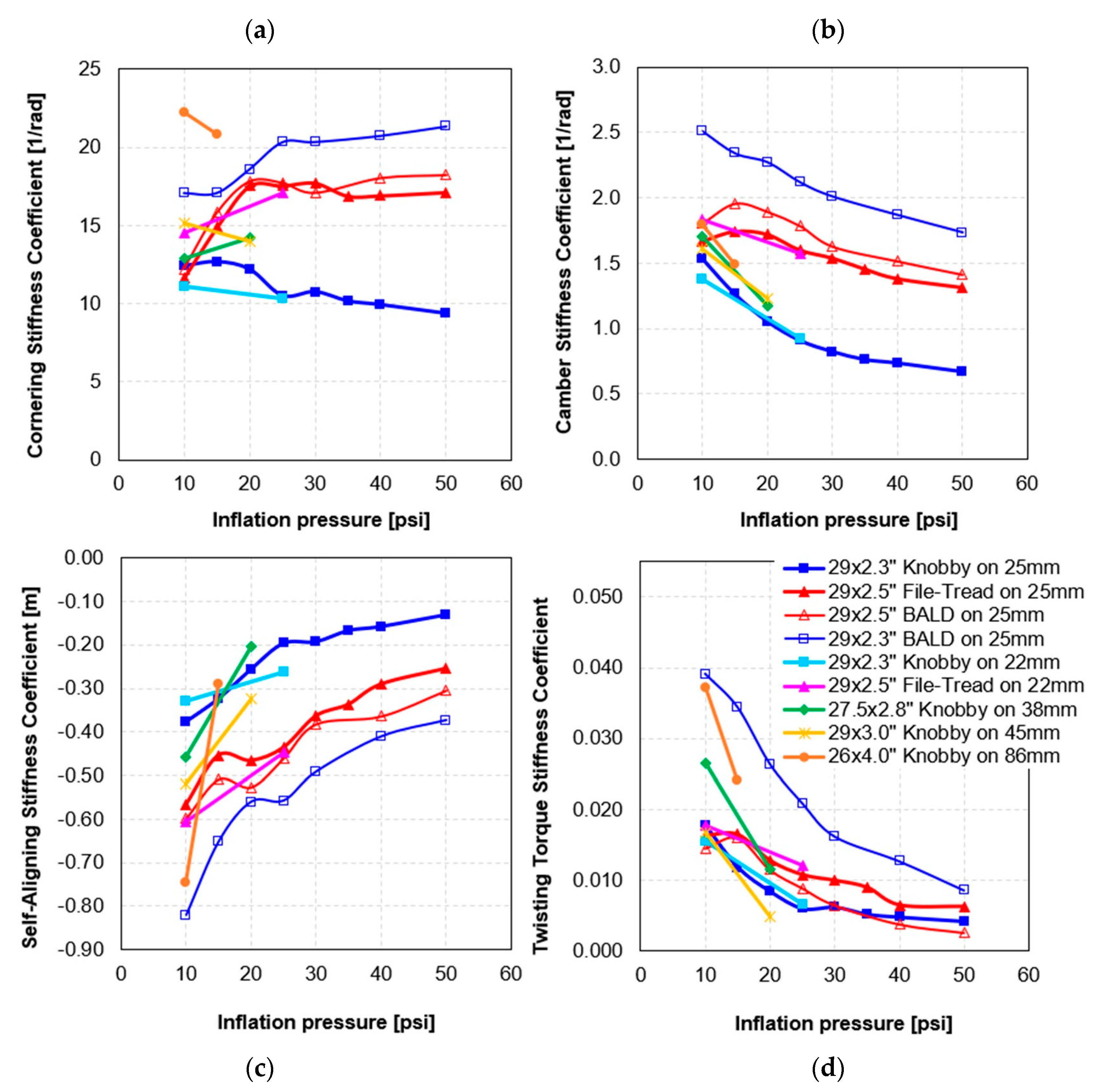
Figure 18.
Knob, tread, bald carcass, measured, and calculated total tire stiffness, and knob count for 29 × 2.3” knobby tire comparing stiffness magnitudes across inflation pressures.
Figure 18.
Knob, tread, bald carcass, measured, and calculated total tire stiffness, and knob count for 29 × 2.3” knobby tire comparing stiffness magnitudes across inflation pressures.


Table 1.
Imperial-based marketing size versus European Tyre and Rim Technical Organisation (ETRTO) designation.
Table 1.
Imperial-based marketing size versus European Tyre and Rim Technical Organisation (ETRTO) designation.
| Tire Size (in) | ETRTO (mm) |
|---|---|
| 29 × 2.3” | 58–622 |
| 29 × 2.5” | 63–622 |
| 29 × 3.0” | 76–622 |
| 27.5 × 2.8” | 71–584 |
| 26 × 4.0” | 102–559 |
© 2020 by the authors. Licensee MDPI, Basel, Switzerland. This article is an open access article distributed under the terms and conditions of the Creative Commons Attribution (CC BY) license (http://creativecommons.org/licenses/by/4.0/).
Share and Cite
MDPI and ACS Style
Dressel, A.; Sadauckas, J. Characterization and Modelling of Various Sized Mountain Bike Tires and the Effects of Tire Tread Knobs and Inflation Pressure. Appl. Sci. 2020, 10, 3156. https://doi.org/10.3390/app10093156
AMA Style
Dressel A, Sadauckas J. Characterization and Modelling of Various Sized Mountain Bike Tires and the Effects of Tire Tread Knobs and Inflation Pressure. Applied Sciences. 2020; 10(9):3156. https://doi.org/10.3390/app10093156
Chicago/Turabian StyleDressel, Andrew, and James Sadauckas. 2020. "Characterization and Modelling of Various Sized Mountain Bike Tires and the Effects of Tire Tread Knobs and Inflation Pressure" Applied Sciences 10, no. 9: 3156. https://doi.org/10.3390/app10093156
Note that from the first issue of 2016, this journal uses article numbers instead of page numbers. See further details here.