Optimisation of Energy Transfer in Reluctance Coil Guns: Application to Soccer Ball Launchers

 , ,
, ,
Abstract
1. Introduction
- Chemical propulsion: mainly used for propelling weapons or rockets; chemical propulsion uses the product of a chemical explosive or expanding reaction to push out a projectile [1]. The benefit of this propulsion is to have a high density of energy stored in a small size as a chemical product leading to strong accelerations, without the need of being connected to a power supply. Its drawback is that the propulsion is a single shot one due to the chemical reaction.
- Mechanical propulsion: there are many types of mechanical propulsion systems. Among the solutions allowing a strong acceleration of the payload are the inertial launchers. They are mostly using an energy storage in heavy high speed rotating mechanical parts such as iron cylinders. These parts are accelerated slowly by a standard motor and part of the stored energy is transferred in a very short amount of type to a projectile by friction. These systems are very simple but their size is much more important than the size of chemical or electromagnetic launchers for a given propelling strength. An example is presented later in this paper.
- Rail Gun propulsion: a rail gun is composed of a pair of conductive parallel rails connected to a direct current (DC) power supply. The electrical circuit is a closed sliding conductor where a payload is placed. Once current flows through the rails, a Lorentz force is created, accelerating the payload to launch it. This propulsion technique is very efficient, and output speed can be higher than using a conventional chemical propulsion as shown in [1], for a launching structure having the same overall size. Compared with chemical propulsion, this solution can be far less expensive than chemical propulsion for launching limited size payloads such as small satellites [2]. However, the presence of a mechanical contact between the rails and the payload propeller can lead to several issues reducing the energy transfer, such as friction losses [3] and plasma phenomena at very high speeds [2,4].
- Coil Gun propulsion: a coil gun is an electromagnetic launcher (EML) converting electricity into kinetic energy using coils [5,6]. There are two types of coil guns. The first one is based on induction to accelerate a conductive non-magnetic projectile using eddy currents induced in a conductive/non-magnetic moving rod inside a magnetic field created by a fixed coil [7]. This solution has an important drawback due to magnetic losses leading to heat generation and controllability loss. The second one is based on accelerating a magnetic projectile by minimizing the reluctance between the projectile and a magnetic field generated by a current flowing through a fixed coil [8]. This type of coil gun, also named reluctance accelerator is simpler to drive than induction coil guns and is very compact.
1.1. Comparison of Existing Soccer Ball Launching Systems
1.2. Reluctance Coil Guns: A Ball Launcher That Can Be Optimized
- Section 2 recalls the principles of coil guns.
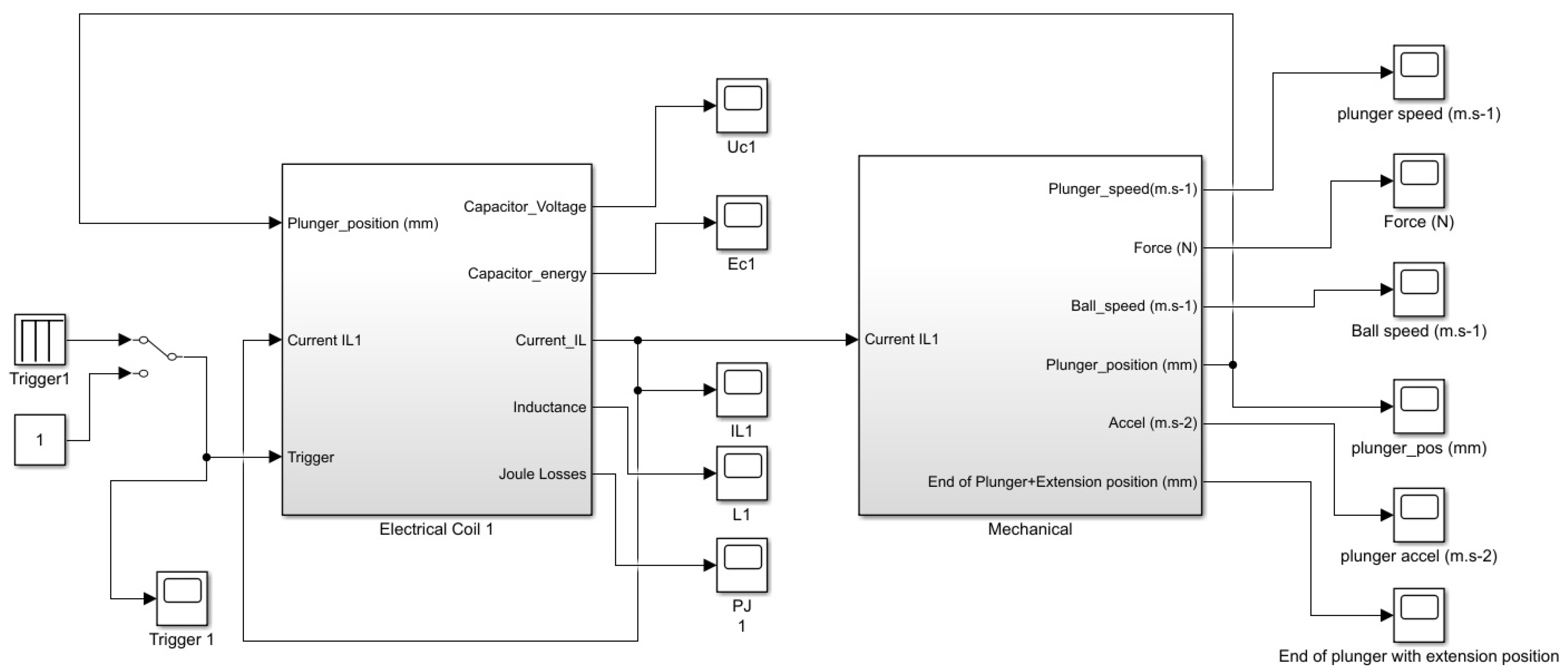
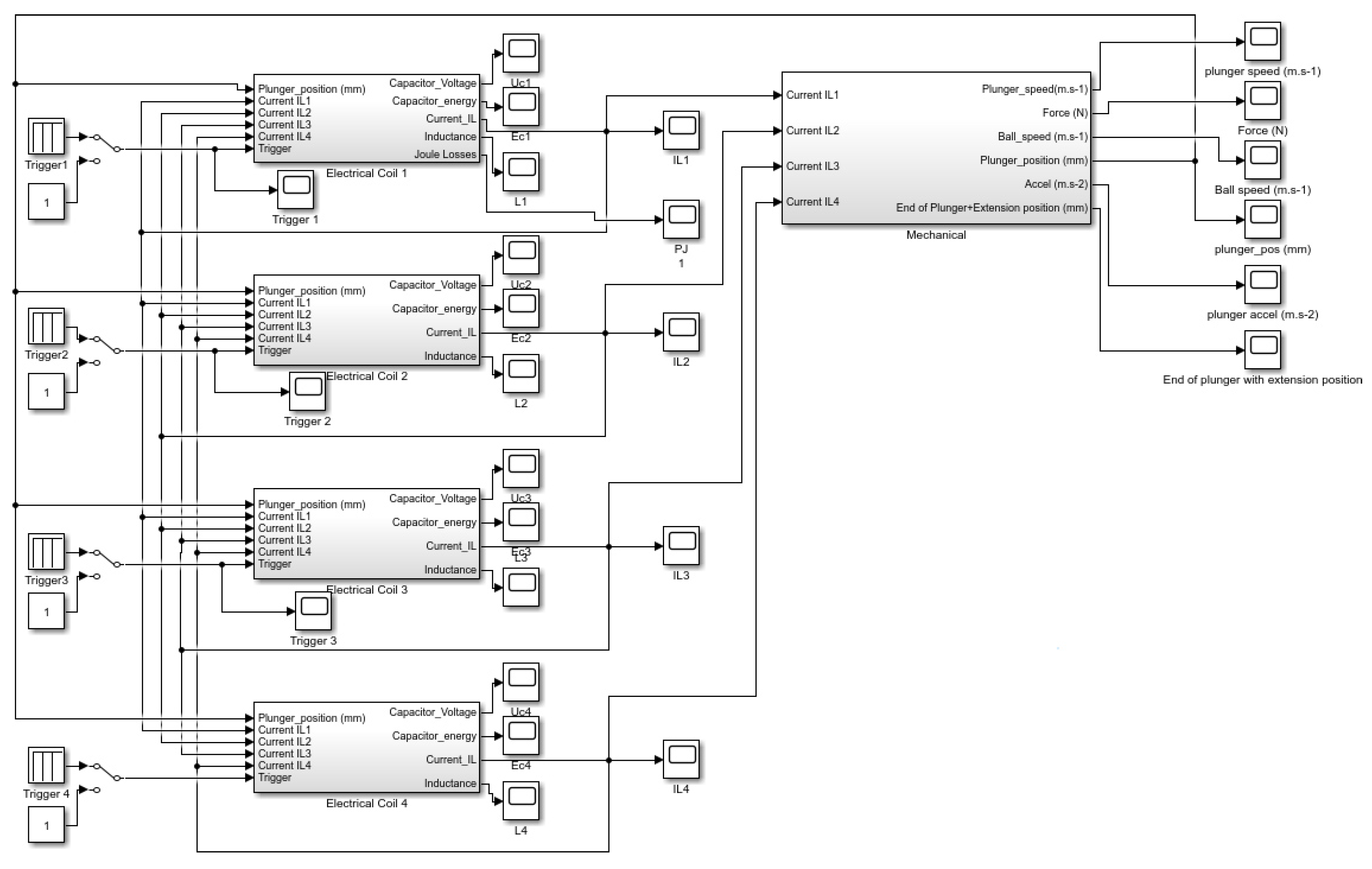
- Section 3 describes 4 mechatronic coupled models of reluctance coil guns. All these coil guns use the same coil copper quantity and have the same overall electrical energy storage capacitance, but they have, respectively, one, two, three and four coils. The electromagnetic part of each model has been implemented using FEMM 4.1, a finite element electromagnetic simulation tool, and Matlab Simulink is used for modelling the electrical and mechanical parts.
- Section 4 presents results, which are discussed in order to conclude on the most relevant coil structure for maximizing the ball speed and the energy transfer of the reluctance coil gun, while maintaining a high level of robustness.
2. Principles of Coil Guns
2.1. Physical Concept
- I: current in the coil (A)
- N: number of turns of the coil
- : flux (Wb)
- R: reluctance (H)
- H·m: permeability of vacuum
- : relative magnetic permeability
- S: cross-sectional area of the circuit (m)
- l: length of the magnetic circuit (m)
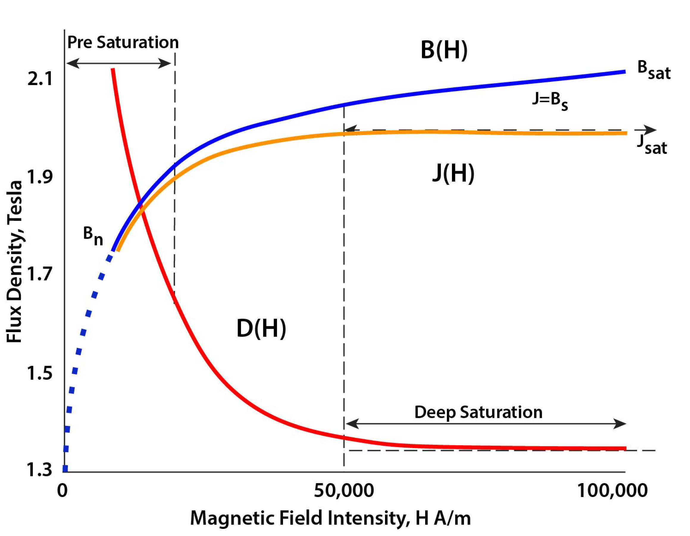
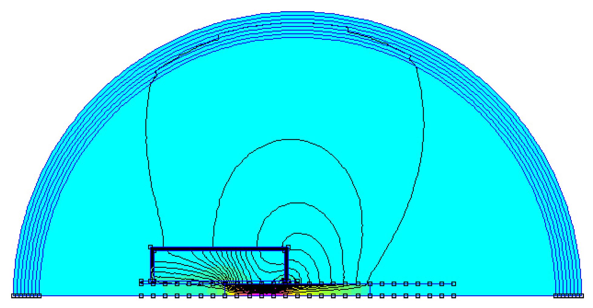
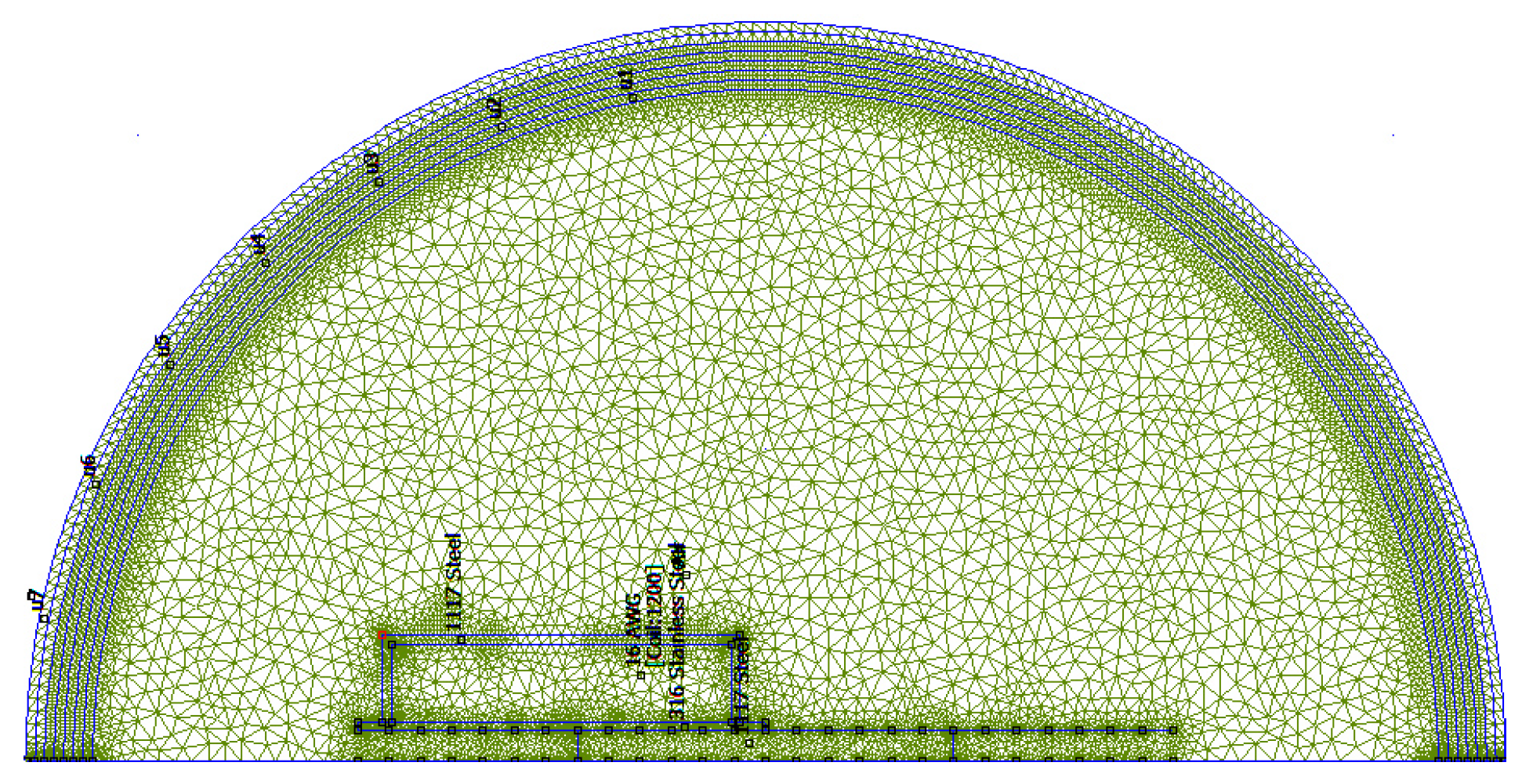
2.2. Electromagnetic Theory and Simulation Software
- The impact of the plunger position leading to change locally the relative magnetic permittivity by a factor 5000 or more.
- One coil: 180 combinations—15 min
- Two coils: 1080 combinations—90 min
- Three coils: 6480 combinations—9 h
- Four coils: 38,880 combinations—54 h
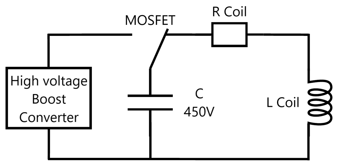
2.3. Electrical Model
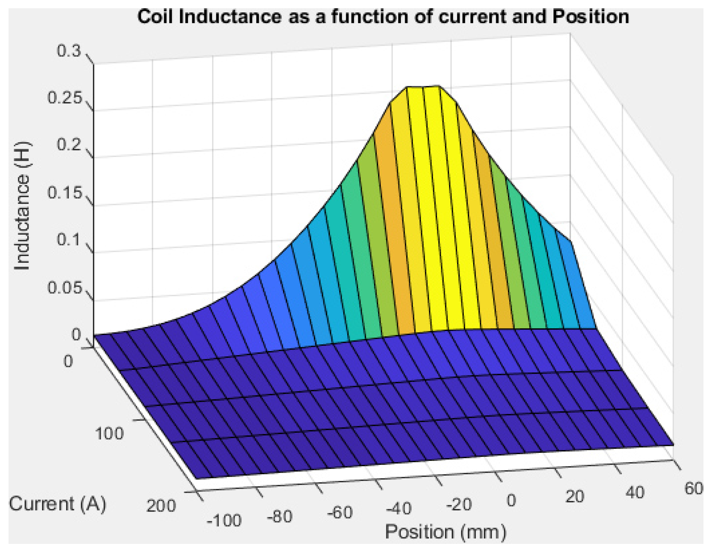
- Inductance value L increases as the plunger enters the coil, is maximized when the plunger centre is aligned with the coil centre, and decreases after that. This is because the magnetic field is well guided when the plunger is inside the coil with a low air gap.
- The inductance value is highly dependent on the coil current. For a current A, L varies, depending on plunger position, from mH to mH whereas for a current A, L varies only from mH to mH. There is an important difference between maximal values because at a low current, magnetic material is not saturated, leading to a high inductance value. In contrast, there is no difference between minimal values because when the plunger is outside the coil, the air gap is so important that it leads to a huge reluctance in the air gap part which prevents saturation of the magnetic circuit.
2.4. Mechanical Model
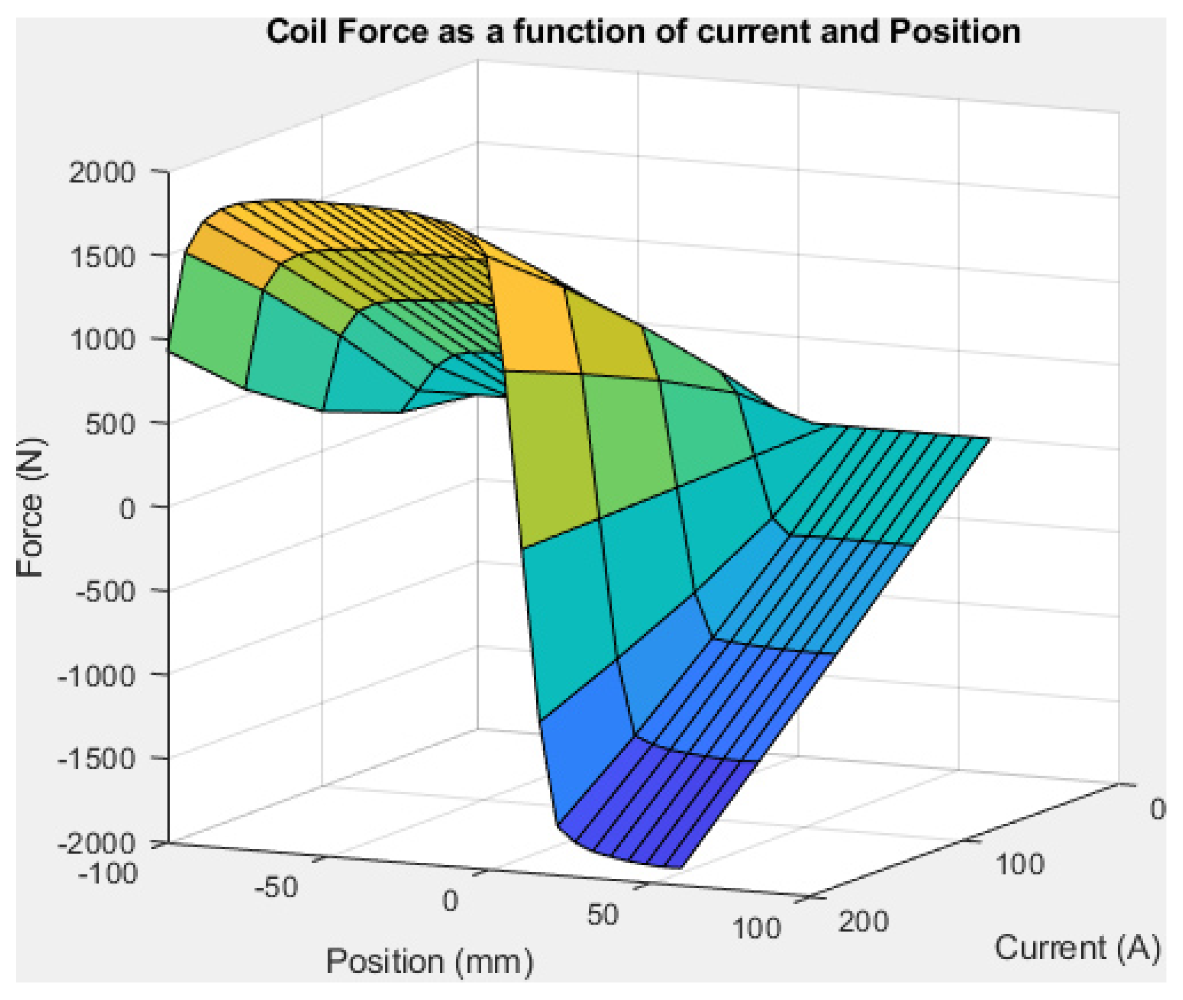
- Force F is almost linear with coil current in any situation.
- Force F is highly dependent on the plunger position. For a current A, F varies, depending on plunger position, from N to N, with N when the plunger is exactly aligned with the centre of the coil. This is because magnetic flux tends to be maximized in a magnetic circuit, leading to reduce the air gap. Consequently, as shown in Figure 16, the magnetic force on the plunger is symmetrical around the point where the centre of the plunger is aligned with the centre of the coil. Thus, it is important to stop powering the coil as soon as the plunger has crossed the coil.
- Force is very small if the plunger is outside the coil. This is normal considering the important length of the air gap replacing the plunger for looping back the magnetic circuit. We can also note that when the plunger is at the centre of the coil, force is null for any value of the current because magnetic flux can not be maximized.
3. Mixed Electrical and Mechanical Model of the Reluctance Coil Gun
3.1. Electrical Model
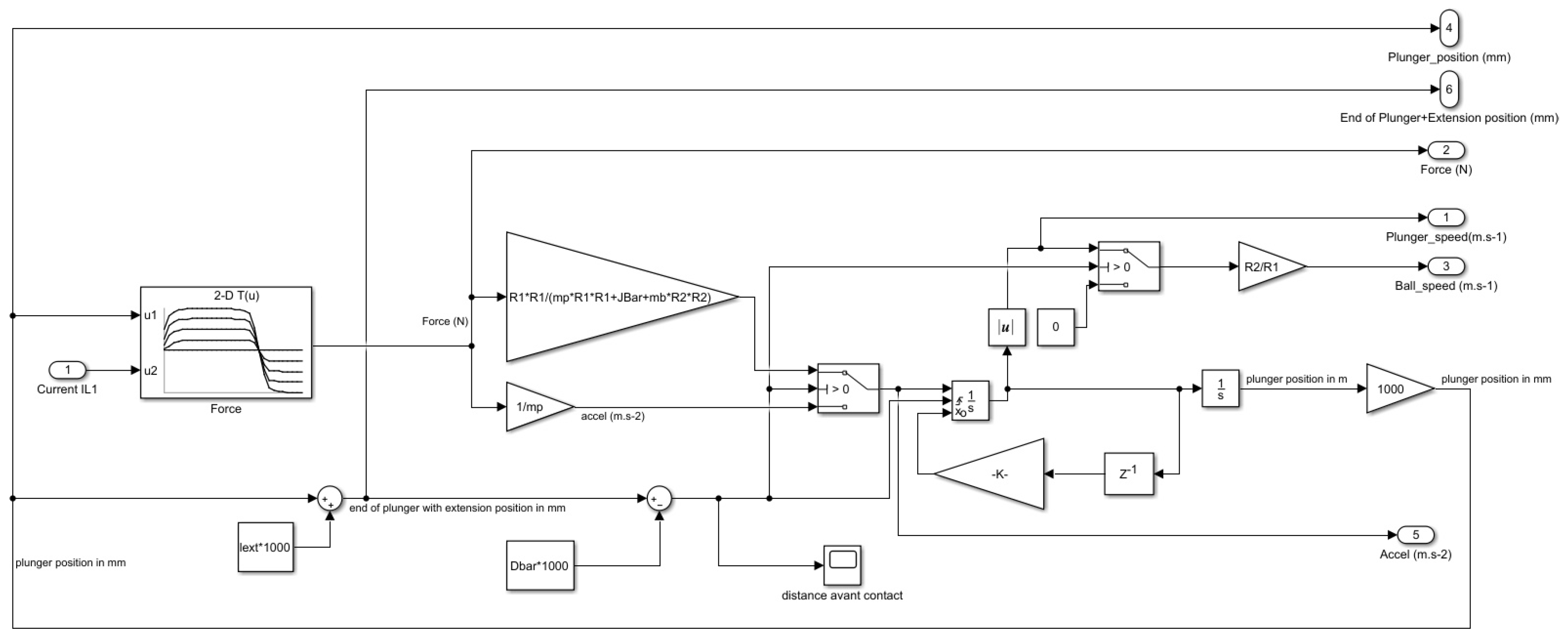
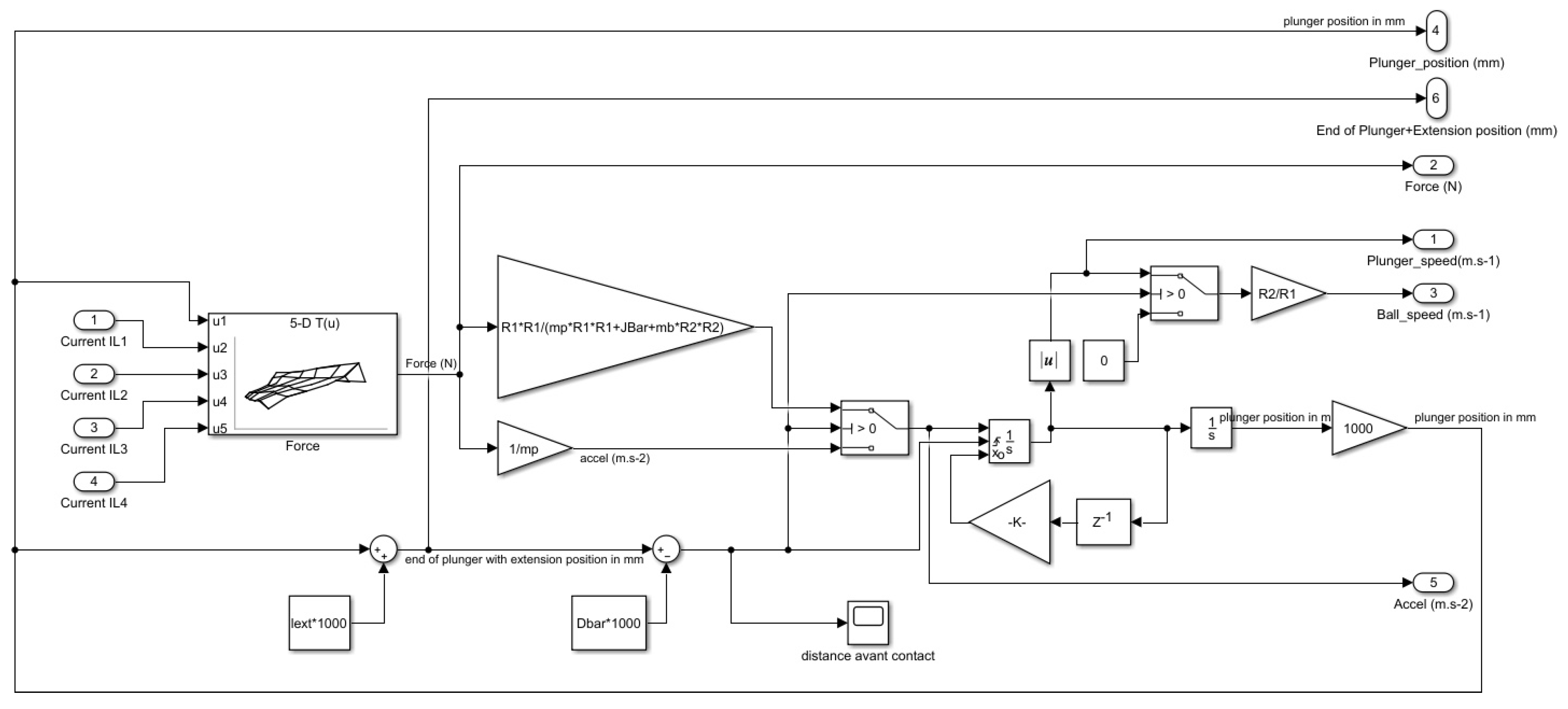
3.2. Mechanical Model
- Phase 1: Acceleration of the plunger without contact on the lever, due to the magnetic force as shown in Equation (2) without contact on the lever. Force depends non-linearly on plunger position and current I. A look-up table (LUT) interpolates linearly the value of F using the simulations performed with FEMM 4.2.
- Phase 2: Impact on the lever corresponding to an elastic shock when plunger hits it at a distance from its rotation centre. Kinetic energy is conserved as described in Equation (3).where is the inertial moment of the lever, and the distances between the lever axis and respectively the plunger impact point and the ball impact point as shown in Figure 15. This leads to a plunger speed just after the shock equal to the given in Equation (4).
- Phase 3: the plunger is accelerated in contact with the lever, which is also in contact with the ball. This means that the lever applies a force on the plunger in subtraction of the magnetic force as shown in Equation (5). This force is an inertial one due to the acceleration of the ball and the lever as shown in Equation (6). It is important to note that theoretically, the speeds of the ball, lever and plunger are not equal after the shock, but in reality they are due to the elastic deformation of the ball as shown in the slow motion picture in Figure 22.wherewith:For small angles, , this leads to:

4. Reluctance Coil Gun Simulations
4.1. Hypothesis
4.2. Model Parameters
- Distance from lever axis to plunger touch point: cm
- Distance from lever axis to ball touch point: cm
- Coils number (each coil as been chosen identical):
- Coils length (for each coil): cm
- Coils number of turns (for each coil): turns
- Coils resistance (for each coil):
- Capacitors number:
- Capacitors value (for each capacitor): 4700 F/
- Capacitors charge voltage: 425 V
- Plunger iron rod diameter: mm
- Plunger iron rod length: cm
- Plunger iron rod mass: g
- Plunger extension diameter: mm
- Plunger extension length: cm
- Plunger extension mass: (in m)
- Distance from coil to lever: cm
- Vertical lever mass: g
- Ball mass: g
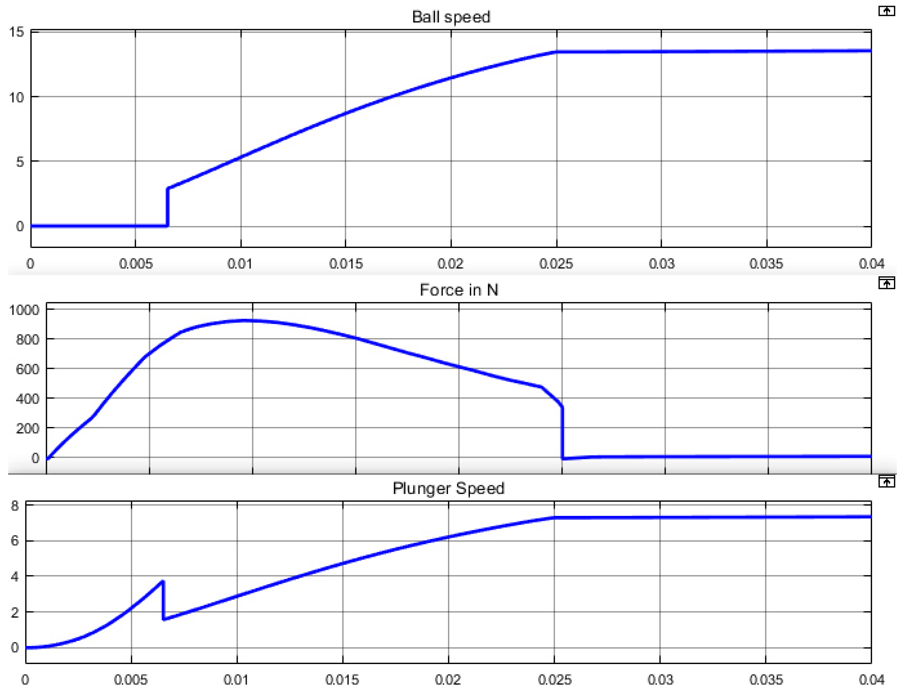
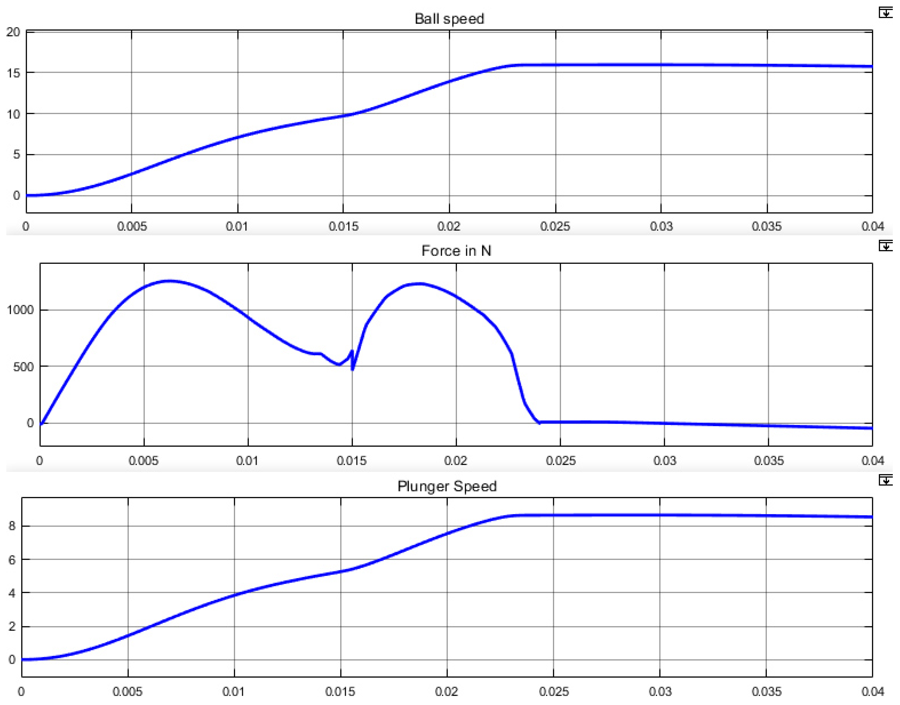
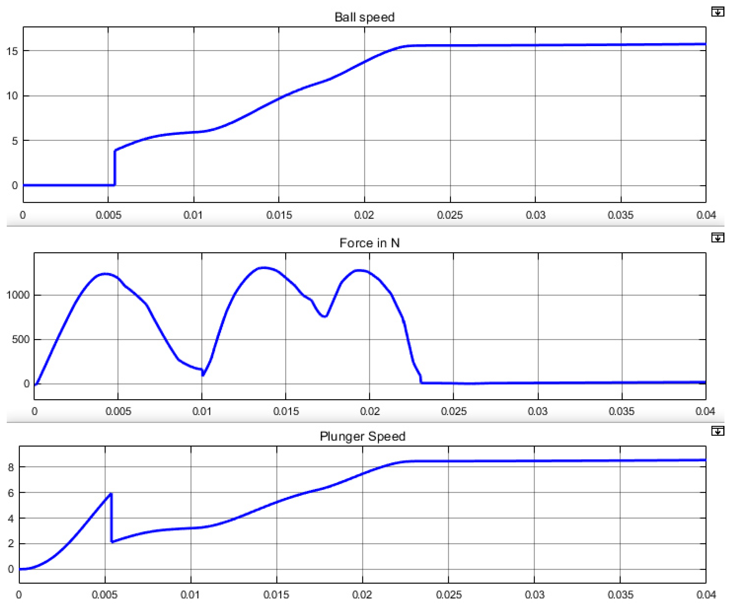
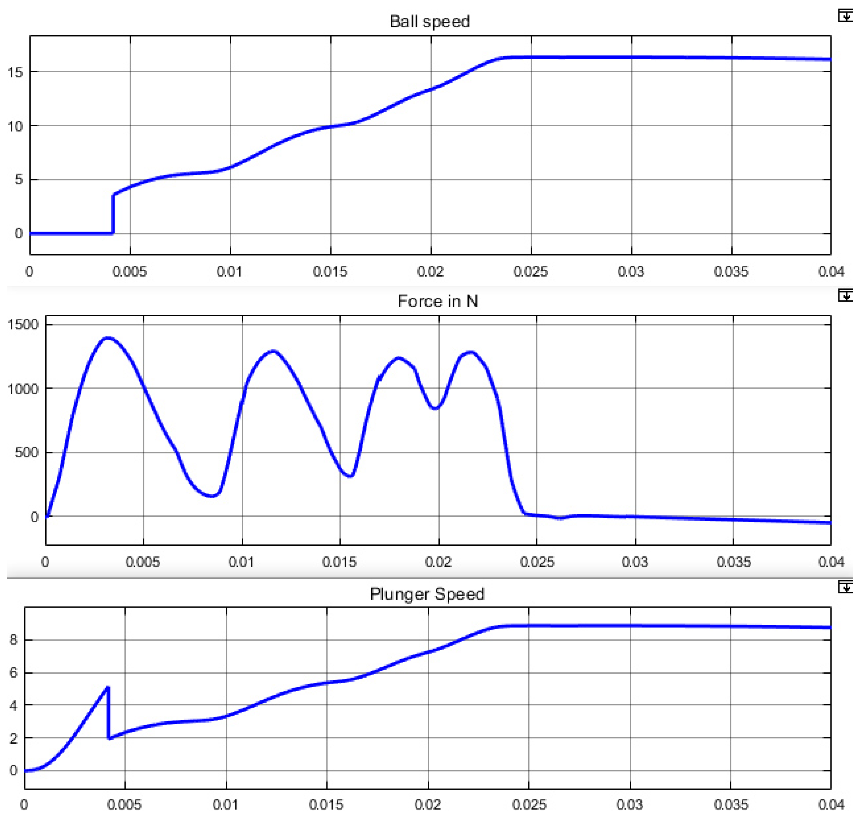
4.3. Simulations
5. Results and Discussion
5.1. Discussion on Simulation Results
5.1.1. Impact of the Coil Gun Structure
5.1.2. Comparison between the Reference Case and the Chosen Configuration
5.1.3. Impact of a Variation of the Coil Triggering Instants
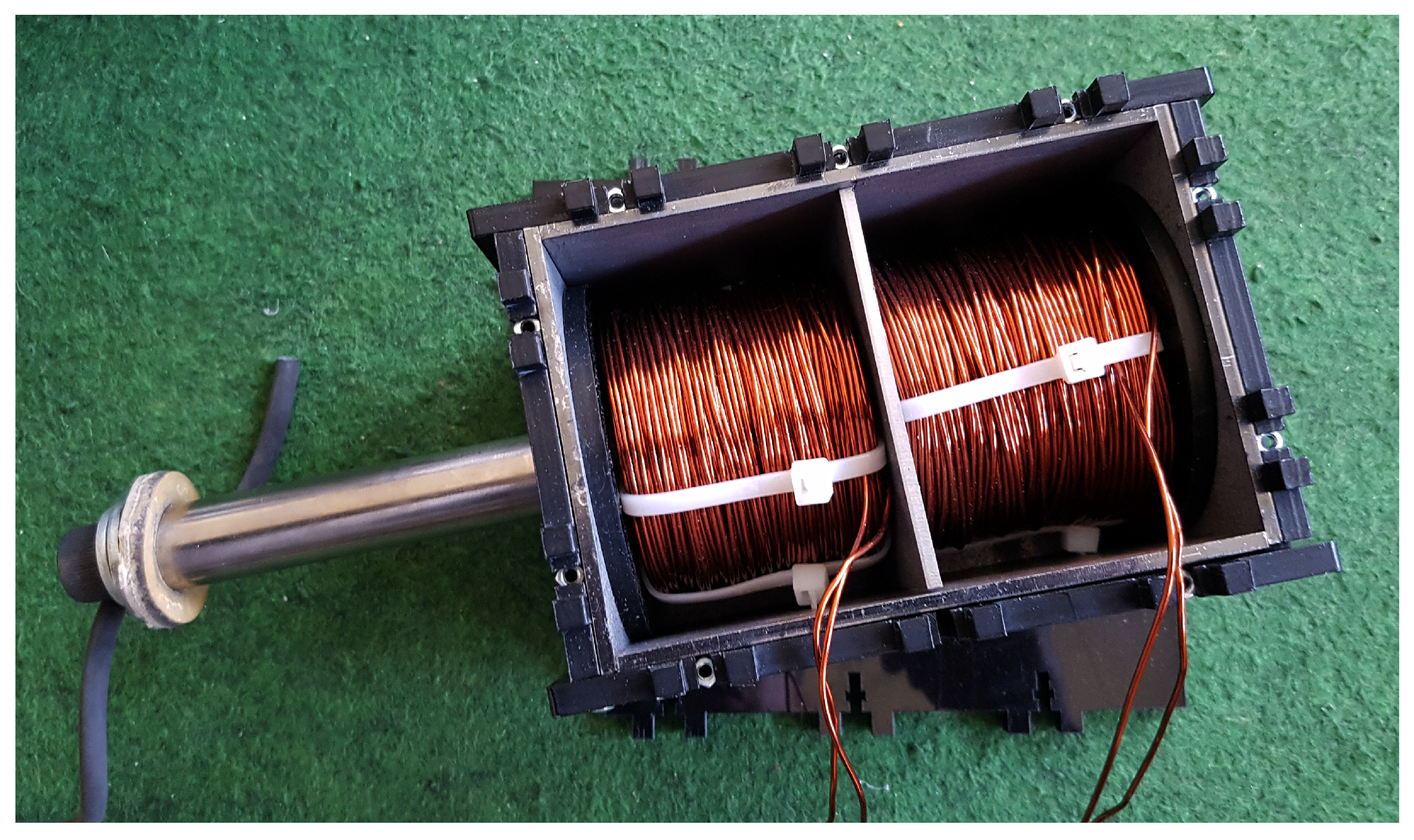
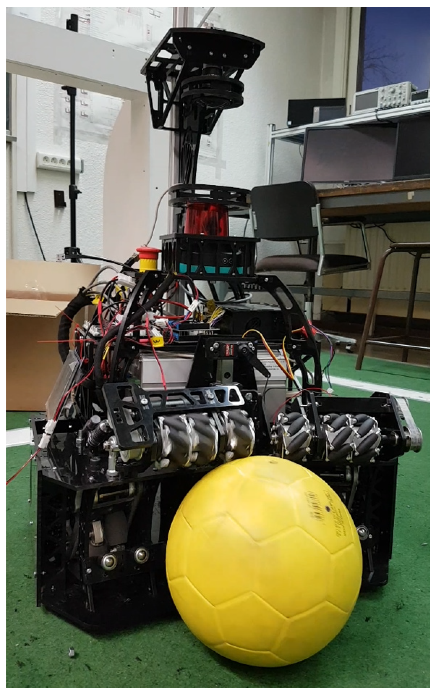
5.2. Experimental Results
6. Conclusions
- Using a two-coil EML is energetically more efficient than the reference situation of an existing coil gun [11], without adding too much mechanical, electrical and algorithmic complexity to the EML. As shown in Table 5, it is also ten times more efficient than a human considering the ball energy to launcher volume ratio.
- Having a high number of coils is not necessary for optimizing the energy transfer. In our case, having two coils in the EML is an excellent trade-off between energy transfer optimization and system complexity.
- Robustness in terms of sensitivity to the coil triggering instants decreases with the number of coils.
Author Contributions
Funding
Acknowledgments
Conflicts of Interest
References
- Tzeng, J.T.; Schmidt, E.M. Comparison of Electromagnetic and Conventional Launchers Based on Mauser 30-mm MK 30-2 Barrels. IEEE Trans. Plasma Sci. 2011, 39, 149–152. [Google Scholar] [CrossRef]
- McNab, I. Progress on Hypervelocity Railgun Research for Launch to Space. IEEE Trans. Magn. 2009, 45, 381–388. [Google Scholar] [CrossRef]
- Cao, B.; Guo, W.; Ge, X.; Sun, X.; Li, M.; Su, Z.; Fan, W.; Li, J. Analysis of Rail Erosion Damage during Electromagnetic Launch. IEEE Trans. Plasma Sci. 2017, 45, 1263–1268. [Google Scholar] [CrossRef]
- Wetz, D.; Stefani, F.; McNab, I. Experimental Results on a 7-m-Long Plasma-Driven Electromagnetic Launcher. IEEE Trans. Plasma Sci. 2011, 39, 180–185. [Google Scholar] [CrossRef]
- Orbach, Y.; Oren, M.; Golan, A.; Einat, M. Reluctance Launcher Coil-Gun Simulations and Experiment. IEEE Trans. Plasma Sci. 2019, 47, 1358–1363. [Google Scholar] [CrossRef]
- Meessen, K.J.; Paulides, J.J.H.; Lomonova, E.A. Analysis and design of a slotless tubular permanent magnet actuator for high acceleration applications. J. Appl. Phys. 2009, 105, 07F110. [Google Scholar] [CrossRef]
- Bencheikh, Y.; Ouazir, Y.; Ibtiouen, R. Analysis of capacitively driven electromagnetic coil guns. In Proceedings of the XIX International Conference on Electrical Machines—ICEM 2010, Rome, Italy, 6–8 September 2010; pp. 1–5. [Google Scholar]
- Abdo, T.M.; Elrefai, A.L.; Adly, A.A.; Mahgoub, O.A. Performance analysis of coil gun electromagnetic launcher using a finite element coupled model. In Proceedings of the 2016 Eighteenth International Middle East Power Systems Conference (MEPCON), Cairo, Egypt, 27–29 December 2016; pp. 506–511. [Google Scholar] [CrossRef]
- Schempf, H.; Kraeuter, C.; Blackwell, M. Roboleg: A robotic soccer-ball kicking leg. In Proceedings of the 1995 IEEE International Conference on Robotics and Automation, Nagoya, Japan, 21–27 May 1995; Volume 2, pp. 1314–1318. [Google Scholar] [CrossRef]
- Vahidi, M.; Moosavian, S. Dynamics of a 9-DoF robotic leg for a football simulator. In Proceedings of the 2015 3rd RSI International Conference on Robotics and Mechatronics (ICROM), Tehran, Iran, 7–9 October 2015; pp. 314–319. [Google Scholar] [CrossRef]
- Meessen, K.J.; Paulides, J.J.H.; Lomonova, E.A. A football kicking high speed actuator for a mobile robotic application. In Proceedings of the IECON 2010—36th Annual Conference on IEEE Industrial Electronics Society, Glendale, AZ, USA, 7–10 November 2010; pp. 1659–1664. [Google Scholar] [CrossRef]
- Gies, V.; Soriano, T. Modeling and Optimization of an Indirect Coil Gun for Launching Non-Magnetic Projectiles. Actuators 2019, 8, 39. [Google Scholar] [CrossRef]
- Williamson, S.; Horne, C.D.; Haugh, D.C. Design of pulsed coil guns. IEEE Trans. Magn. 1995, 31, 516–521. [Google Scholar] [CrossRef]
- Kang, Y. A high power-density, high efficiency front-end converter for capacitor charging applications. In Proceedings of the Applied Power Electronics Conference and Exposition (APEC 2005), Austin, TX, USA, 6–10 March 2005; Volume 2, pp. 1258–1264. [Google Scholar] [CrossRef]
- Rao, D.K.; Kuptsov, V. Effective Use of Magnetization Data in the Design of Electric Machines with Overfluxed Regions. IEEE Trans. Magn. 2015, 51, 1–9. [Google Scholar] [CrossRef]
- Lequesne, B.P. Finite-element analysis of a constant-force solenoid for fluid flow control. IEEE Trans. Ind. Appl. 1988, 24, 574–581. [Google Scholar] [CrossRef]
- SMIOT: Scientific Microsystems for the Internet of Things. 2019. Available online: http://www.smiot.fr (accessed on 2 March 2020).


| Launcher | Length | Width | Height | Volume | Weight | Ball Speed | Ball Energy | |
|---|---|---|---|---|---|---|---|---|
| (cm) | (cm) | (cm) | (cm) | (kg) | (m·s) | (J) | (J·dm) | |
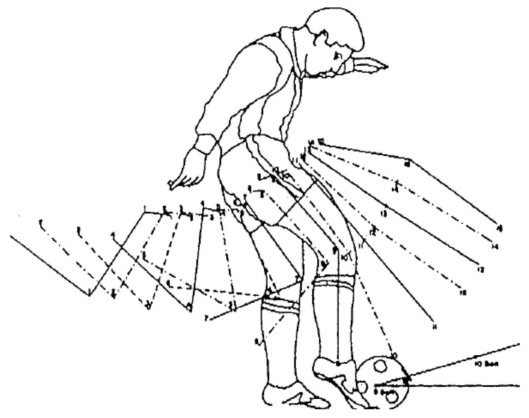
| Soccer player leg | 160 | 20 | 80 | 20 | 36 | 290 | 2.18 | |
| Rotating inertial launcher | 25 | 65 | 25 | 25 | 29 | 190 | 4.75 | |
| Robot arm [9] | 240 | 240 | 30 | 50 | 21 | 100 | 0.07 | |
| Reluctance coil gun [11] | 30 | 9 | 9 | 4.5 | 11.4 | 29 | 12.08 |
| Number of Coils | 1 | 2 | 3 | 4 |
| Optimized Ball Speed (m·s) | 13.5 | 16 | 16.1 | 16.3 |
| Kicking Range (m) | 18.6 | 26.1 | 26.4 | 27 |
| Triggering Instant (ms) | 7 | 8 | 9 | 10 | 11 | 12 | 13 |
| Optimized Ball Speed (m·s) | 14.4 | 15.2 | 15.8 | 16.1 | 16 | 15.8 | 15.6 |
| Triggering Instant (ms) | 13.5 | 14.5 | 15.5 | 16.5 | 17.5 |
| Optimized Ball Speed (m·s) | 13.3 | 14.6 | 16.4 | 14.3 | 13.9 |
| Launcher | Length | Width | Height | Volume | Weight | Ball Speed | Ball Energy | |
|---|---|---|---|---|---|---|---|---|
| (cm) | (cm) | (cm) | (cm) | (kg) | (m·s) | (J) | (J·dm) | |
| Soccer player leg | 160 | 20 | 80 | 20 | 36 | 290 | 2.18 | |
| Rotating inertial launcher | 25 | 65 | 25 | 25 | 29 | 190 | 4.75 | |
| Robot arm [9] | 240 | 240 | 30 | 50 | 21 | 100 | 0.07 | |
| Reluctance coil gun [11] | 30 | 9 | 9 | 4.5 | 11.4 | 29 | 12.08 | |
| Optimized coil gun | 30 | 9 | 9 | 4.5 | 16.4 | 60.5 | 25.21 |
© 2020 by the authors. Licensee MDPI, Basel, Switzerland. This article is an open access article distributed under the terms and conditions of the Creative Commons Attribution (CC BY) license (http://creativecommons.org/licenses/by/4.0/).
Share and Cite
Gies, V.; Soriano, T.; Marzetti, S.; Barchasz, V.; Barthelemy, H.; Glotin, H.; Hugel, V. Optimisation of Energy Transfer in Reluctance Coil Guns: Application to Soccer Ball Launchers. Appl. Sci. 2020, 10, 3137. https://doi.org/10.3390/app10093137
Gies V, Soriano T, Marzetti S, Barchasz V, Barthelemy H, Glotin H, Hugel V. Optimisation of Energy Transfer in Reluctance Coil Guns: Application to Soccer Ball Launchers. Applied Sciences. 2020; 10(9):3137. https://doi.org/10.3390/app10093137
Chicago/Turabian StyleGies, Valentin, Thierry Soriano, Sebastian Marzetti, Valentin Barchasz, Herve Barthelemy, Herve Glotin, and Vincent Hugel. 2020. "Optimisation of Energy Transfer in Reluctance Coil Guns: Application to Soccer Ball Launchers" Applied Sciences 10, no. 9: 3137. https://doi.org/10.3390/app10093137
APA StyleGies, V., Soriano, T., Marzetti, S., Barchasz, V., Barthelemy, H., Glotin, H., & Hugel, V. (2020). Optimisation of Energy Transfer in Reluctance Coil Guns: Application to Soccer Ball Launchers. Applied Sciences, 10(9), 3137. https://doi.org/10.3390/app10093137