Abstract
As a classic inerter system, the tuned viscous mass damper (TVMD) has been proven to be efficient for vibration control. It is characterized by an amplification effect, where the deformation of the dashpot in the TVMD can be larger than that of a single dashpot, providing enhanced energy dissipation. However, the contribution of this system to the enhancement of the energy dissipation quantity and vibration control remains unclear. To deal with this, and considering the underlying soil, this study proposes a systematic energy spectrum analysis framework for the single-degree-of-freedom (SDOF) element controlled by a tuned viscous mass damper (TVMD) in order to reveal the energy characteristics of the TVMD and develop an optimal energy dissipation enhancement-based design. The proposed energy spectrum analysis includes ground motion propagation and energy balance analysis. Considering the underlying soil, energy balance analysis is performed for a series of SDOF elements connected to the TVMD, which yields a fitted input energy spectrum for optimal design of the TVMD. Extensive parametric analysis reveals energy characteristics of the TVMD compared with a single dashpot, yielding an optimal energy dissipation enhancement-based design. The findings of this study show that by considering the soil underneath the inerter-based structure, the developed energy spectrum analysis quantifies the degree of energy dissipation enhancement effect of the TVMD. The proposed design is effective in guaranteeing the target of displacement control, which optimizes the efficiency and quantity of the TVMD for energy dissipation, relieving the energy-dissipation burden on the primary element.
1. Introduction
Passive control technology has been proven to be an efficient way to achieve vibration control for aseismic structures, especially inerter-based vibration control devices. Such technology has attracted significant attention [1,2,3,4] owing to its apparent mass amplification and negative stiffness effects. Inerters are inertial elements with two terminals that develop an acceleration-dependent force that is proportional to a constant (inertance), which assumes mass units [5,6,7]. Their apparent mass amplification effect refers to the fact that the inertance can be thousands of times greater than the gravitational mass of the inerter [8]. Typical inerters include ball-screw [9], fluid-based [10,11], rack–pinion [12], and electromagnetic [13] mechanisms. Regardless of the physical mechanism employed, the most widely considered inerter systems are tuned viscous mass dampers (TVMDs) [8] and tuned inerter dampers [14]. Other novel mechanical layouts have also been proposed, such as particle inerter systems [15], tuned liquid inerter systems [16], and lightweight tuned inerter mass systems [17,18]. Ikago et al. [8] proposed a TVMD consisting of an inerter incorporating a dashpot in parallel and then in series with a tuning spring. They also pointed out a dashpot-deformation amplification effect, that the deformation of the dashpot in a TVMD can be larger than the entire deformation of the TVMD for enhanced energy dissipation. Zhang et al. [19] derived a closed-form equation to quantify the theoretical relationship between the amplification of dashpot deformation and the key parameters of the inerter system. Pan et al. [20] proposed a displacement demand-oriented design method for an inerter system to achieve the desired seismic performance for primary structures. Zhao et al. [21,22] analyzed the benefits of an isolation system enhanced by a TVMD and developed a multiobjective-based optimal design method.
Reviewing the existing studies referring to TVMDs, performance related to displacement and acceleration has been analyzed extensively [8]. However, from the energy perspective, the advantageous energy dissipation enhancement effect, by which the TVMD exhibits increased energy dissipation capacity compared with a single dashpot, remains unclear. For passive seismic control of structures, energy-based analysis and optimal design are effective solutions for the typical control of dampers [23,24,25,26,27] in earthquake-prone areas. Benavent-Climent et al. [28,29,30] investigated the energy performance of a typical frame and developed a design for hysteretic energy-dissipating devices. Energy spectrum and design curves are efficient approaches to designing such devices, while a rigid foundation is commonly assumed without considering the soil [25,31,32]. As for controlled structures built on deep cover soft deposits, the energy responses calculated by this assumption are not accurate because of the nonlinear soil behavior excited by the ground motion. Seismic ground motions pass from the bedrock through the soil to the ground surface, yielding significant changes in their characteristics and in the energy performance of the controlled structures. In the existing literature, typical representations to simulate the nonlinear dynamic behavior of soil include equivalent linearization [33], elastoplastic dynamic constitutive [34], and viscoelastic dynamic constitutive [35] models. Compared with the simple-form equivalent linearization model and the impractical elastoplastic dynamic constitutive model, a viscoelastic dynamic constitutive model, such as the Davidenkov model, is not only capable of describing the nonlinear behavior of the soil but also convenient for practical application [36].
To quantify the energy dissipation enhancement effect of TVMDs, we developed an energy spectrum analysis framework by considering the soil underlying the inerter-based structure. Ground motion propagation for the bedrock excitation was conducted using the classic Davidenkov model [35] to imitate the nonlinear behavior of the soil. After obtaining the responses of ground motion propagation, energy balance analysis was performed for a series of damped single-degree-of-freedom (SDOF) elements connected to the TVMD with different fundamental periods and TVMD parameters. Fitted seismic input energy spectra were also provided for parametric determination of the TVMD. Following the energy spectrum analysis, extensive parametric analysis was conducted to distinguish the energy working basis of the TVMD compared with the single dashpot, yielding an optimal energy dissipation enhancement-based design. Numerical design cases are given to verify the effectiveness of the proposed design method.
2. Theoretical Analysis of Energy Spectrum Study
2.1. Introduction of SDOF-TVMD System and Underlying Soil
Considering the objective existence of the soil underlying a structure and its vibration during seismic excitation [37,38], a complete energy spectrum analysis consists of conducting ground motion propagation and analyzing the energy balance of a series of SDOF elements. During ground motion propagation for bedrock excitation, one-dimensional analysis is commonly performed, in which the ground motion is approximated by vertically propagating horizontal shear waves through the horizontal soil layers. The mechanical model of horizontal soil layers is approximated as a Kelvin–Voigt solid [39] here, and the soil material is represented by a nonlinear soil dynamic constitutive model, shown in Figure 1.
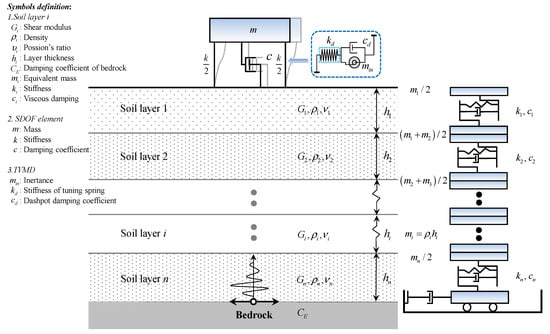
Figure 1.
Lumped parameter model representation of a horizontally layered soil deposit and the aboveground structure.
After obtaining the seismic excitation propagated from the bedrock, energy balance analysis was performed for a series of SDOF elements and SDOF-TVMD systems with different fundamental periods. The detailed analysis procedure and results are presented in the following sections.
2.2. Ground Motion Propagation of the Soil
2.2.1. Davidenkov Model of Soil
For the strong seismic excitations of concern here, the linear elastic solution is not valid, since the soil behavior is inelastic, nonlinear, and strain-dependent. In the condition of increasing shear strain, the shear stiffness decreases rapidly, whereas the load reversal makes the soil experience hysteretic behavior with a percentage of material damping [35]. To deal with this, a nonlinear soil dynamic constitutive model (the Davidenkov model) is recommended [40,41], and was employed in the nonlinear time history analysis.
The dynamic shear modulus ratio () of the Davidenkov model is given by [35]:
where is the dynamic secant shear modulus, is the maximum shear modulus, is the dynamic shear strain, and , , and are the fitting parameters related to soil properties. Given these, the stress–strain skeleton curve of the Davidenkov model can be expressed as follows:
The stress–strain hysteresis curve of the Davidenkov model is given by the following equation:
where and are the values of soil shear stress and shear strain at the last load reversal, respectively. To illustrate this model intuitively, its dynamic shear stress–shear strain curves are plotted in Figure 2, taking as an example.
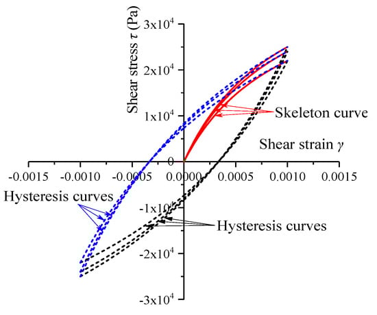
Figure 2.
Dynamic shear stress–shear strain curves of the Davidenkov model.
By deriving in Equations (2) and (3), the tangent shear modulus of the stress-strain curves, , can be given as follows:
where superscript and represent values at the end of the previous and current increment, respectively.
2.2.2. Equation of Ground Motion Propagation
The equation of motion for vertically propagating ground motion through an unbounded soil medium can be written as follows:
where , , , and are the density, shear stress, shear modulus, and shear strain of the soil, respectively. Additionally, is the soil displacement, is the depth from the ground surface, and is the viscosity constant.
From Equation (5), we can obtain the following:
In time domain analysis, nonlinear analysis can be used to capture the cyclic behavior of soil. In this approach, the equations of motion and equilibrium are solved in discrete time increments. The ground motion propagation equation, Equation (6), is written as follows:
where , , and are the soil-nodal vectors of relative displacement, relative velocity, and relative acceleration, respectively. Additionally, is the acceleration at the base of the soil; is the unit vector; , , and are the matrices of soil mass, soil damping, and soil stiffness, respectively, and these matrices are assembled using the incremental properties of the soil layers given in Figure 1. The properties were obtained from a constitutive model (the Davidenkov model), which describes the cyclic behavior of soil. As shown in Figure 1, each individual layer is represented by a corresponding mass , a nonlinear spring , and a dashpot with a viscous damping coefficient . Lumping together half the mass of each of two consecutive layers at their common boundary forms the mass matrix. The stiffness matrix is updated at each time increment to incorporate the nonlinearity of the soil. At each time increment, stiffness for layer is defined as follows:
where is the current tangent shear modulus and is the thickness of layer . In a nonlinear soil model, soil damping is captured through hysteretic loading–unloading cycles in the soil model. The use of damping matrix may become unnecessary in this instance. The damping matrix may be used as a mathematical convenience or to include damping at very small strains, where the response of many constitutive models is nearly linearly elastic [39].
2.3. Energy Balance Analysis
2.3.1. Introduction of the Inerter
The resisting inertial force of the inerter is ideally proportional to the relative acceleration of the two terminals, and this ratio is called inertance, . Figure 3 shows the mechanical model of the inerter, where and denote the acceleration of the two terminals. The inertial force of the inerter, , can be expressed as .
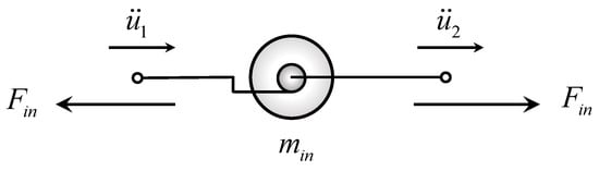
Figure 3.
Mechanical model of the inerter.
2.3.2. Governing Equations
As shown in Figure 4, mechanical models were plotted for the original SDOF element, the SDOF element connected to a single dashpot, and the SDOF element connected to the TVMD. The TVMD consists of a tuning spring in series connection with the configuration of an inerter and a dashpot spaced in parallel. Subject to the base seismic excitation , the differential equation of motion of the original SDOF element can be expressed as follows:
where , , and are the mass, damping coefficient, and stiffness and , , and are the displacement, velocity, and acceleration of the primary SDOF element relative to the ground, respectively. If an extra dashpot is inserted between the mass and the ground for vibration control, the added damping coefficient is added to to modify the governing equation.
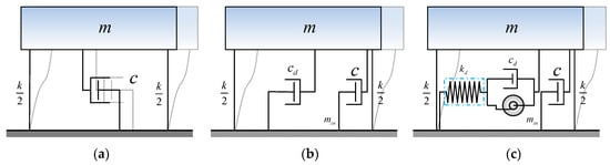
Figure 4.
Mechanical models of the analyzed structures: (a) original single-degree-of-freedom (SDOF) element; (b) SDOF element connected to a single dashpot; (c) SDOF element connected to the tuned viscous mass damper (TVMD).
In terms of the SDOF element connected to the TVMD, an extra degree of freedom, i.e., deformation of the dashpot () is added so that the governing equation is modified as follows:
where and are the velocity and acceleration of the dashpot in the TVMD. The considered control devices, including the single dashpot and the TVMD, can be described in a dimensionless form by the following equation:
where , , and are the inertance–mass ratio, nominal damping ratio, and stiffness ratio, respectively.
2.3.3. Energy Balance Analysis
Widely accepted for energy balance analysis, the relative energy balance equation [25,42,43,44] was used in this study to explore the earthquake input energy spectrum. Considering the damping effect of a single dashpot, by multiplying Equation (9) by and integrating over the entire duration of an earthquake, i.e., from to (here, the subscript f refers to the instant when the earthquake fades away), it can obtained for the original SDOF element:
The right-side term of Equation (12) is conventionally defined as the input energy (), whereas the dissipation energy contributed by the single dashpot and primary SDOF element is defined as and , respectively. To eliminate the influence of mass on the seismic-induced energy spectra, , , and are given as follows:
In addition, the left-side terms of Equation (12), kinetic energy () and elastic strain energy () are defined as and , respectively. However, for a damped elastic SDOF system, and are almost zero at the time when the earthquake vanishes (or when the vibration of the structure stops).
In terms of the SDOF element connected to the TVMD, the energy balance analysis was conducted by multiplying Equation (10) by and integrating over the entire duration of the earthquake:
where the expression of input energy is consistent with the case in Equation (13). The dissipation energy contributed by the dashpot of the TVMD, , and the primary SDOF element, , are changed as follows:
3. Ground Motion Propagation of Nonlinear Soil
3.1. Fitting Parameters and Implementation of Davidenkov Model in ABAQUS
3.1.1. Fitting Parameters of Soil
Adopting the Davidenkov model for this study, the three key parameters , , and in Equation (1) were fitted through the experimental data using a numerical algorithm [45]. Taking three sets of existing experimental data of typical Shanghai soft soils (clay, sand, and muddy clay) as an example [46], the fitting effect is shown in Figure 5. As illustrated in Figure 5, the degradation of the shear modulus with strain and the hysteretic behavior and damping are critical characteristics of soil behavior under cyclic loading. The considered model is effective at capturing this behavior and predicting the values of shear modulus degradation and damping increase with strain. The fitting parameters of the typical Shanghai soft soils in this study are summarized in Table 1.
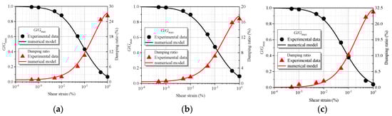
Figure 5.
Comparison between numerical model predictions and experimental data for (a) clay, (b) sand, and (c) muddy clay.

Table 1.
Fitting parameters for different types of soil.
The viscous damping effect of the soil is represented by Rayleigh damping [47,48] and assumed proportional to the stiffness of the soil layers [39]:
where is the circular frequency and takes the fundamental frequency corresponding to the first mode (), is the equivalent damping ratio of the soil, and the value of is between 1.5 and 4% for most soils [39]. Here, is assumed to be independent of the strain level, therefore the effect of hysteretic damping induced by nonlinear soil behavior can be separated from (but added to) viscous damping. The Davidenkov model was incorporated as an independent subroutine attached to ABAQUS (Dassault, Paris, France) [49] by the author to conduct nonlinear ground motion propagation analysis. Details and verification of this subroutine can be found elsewhere [45].
3.1.2. Justification of the Davidenkov Model in Ground Motion Propagation
Before starting the ground motion propagation analysis, a comparison analysis was conducted between the Davidenkov model and the commonly used equivalent linear method, highlighting the necessity of using a nonlinear dynamic constitutive model. Taking bedrock ground motion and a representative soil site as an example [45], the analyzed results of the two methods were obtained, of which the acceleration time history and the Fourier spectrum of input ground motion are shown in Figure 6. Figure 7 illustrates a comparison between acceleration and relative displacement time history responses at the ground surface.
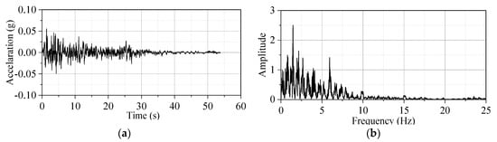
Figure 6.
Input bedrock ground motion: (a) acceleration time history; (b) Fourier spectrum.
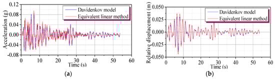
Figure 7.
Comparison of (a) ground surface acceleration time history responses and (b) ground surface relative displacement responses.
In addition, the differences of peak responses and relative differences for five typical ground motions selected from different earthquakes are further calculated and listed in Table 2. As shown in Table 2, the peak ground acceleration responses calculated by the Davidenkov model are less than those by the equivalent linear method, and the mean relative difference of the five records is 17.58%. The peak ground relative displacement responses calculated using the Davidenkov model are also less than those by the equivalent linear method, and the mean relative difference of the five records is 16.17%. The calculation results of the nonlinear dynamic constitutive model are generally smaller than those of the equivalent linear method, which is consistent with previous research [35,50,51] and is necessary to represent the actual behavior of the soil.
Table 2.
Comparison between the Davidenkov model and equivalent linear method results.
Given the need for the Davidenkov model in this study, its accuracy was further justified via a comparison, in which a real bedrock sample (“in-borehole,” 100 m depth below ground surface) and its corresponding ground surface acceleration time history (east–west component of TKCH 080) recorded during the Tokatchi-oki earthquake (2003, Japan) [52] were selected for analysis, as shown in Figure 8. The bedrock acceleration time history was used as input to predict the ground surface acceleration time history, and the computed history is given in Figure 9. It can be seen that the computed time history can predict the recorded time history well. The wave shape of the computed time history is basically the same as that of the recorded time history. Specifically, the peak ground acceleration values of the computed and recorded time history are 0.46 g and 0.49 g, respectively, and the relative difference is 6.12%. In addition, the normalized acceleration response spectrum (characterized by acceleration amplification factor ) of the computed time history was compared with the recorded data, shown in Figure 10. The results show satisfactory agreement with the data, especially the predominant period of the ground surface acceleration time history, as well as the corresponding resonant peaks, where both are well predicted. These results are consistent with previous research [52] and further justify that the use of the Davidenkov model to represent soil behavior is reasonable and accurate.
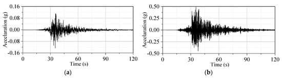
Figure 8.
TKCH 080 acceleration time history records: (a) bedrock; (b) ground surface.
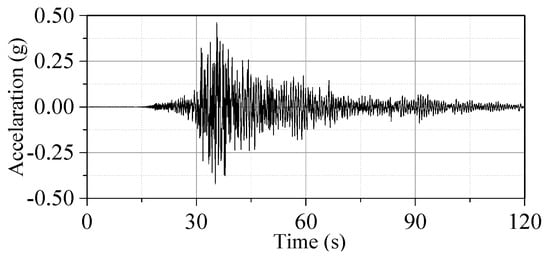
Figure 9.
Computed ground surface acceleration time history.
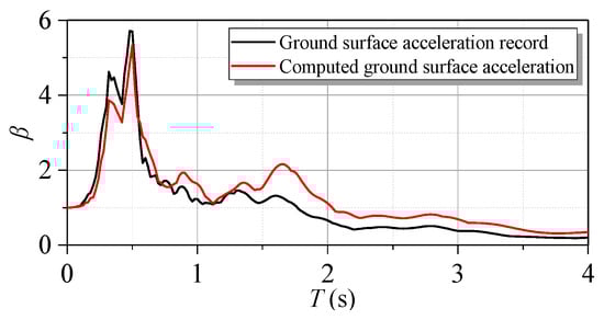
Figure 10.
Comparison of computed and recorded ground surface acceleration response spectra.
3.2. Selection of Typical Soft Deposit and Ground Motion Records
Adopting the Davidenkov model, propagation of ground motion includes determining the deep cover soft deposit and ground motion records. To deal with this, a typical soil site with a thickness of 280 m was selected, designed by Huang et al. [53] based on Shanghai stratigraphic survey data as well as the current Shanghai foundation specifications. The details of the site are listed in Table 3, where is the density of soil, is Poisson’s ratio, and is the shear wave velocity of soil.
Table 3.
Parameters of soil site in urban area of Shanghai. : density; : Poisson’s ratio; : shear wave velocity.
Strong ground motion records measured at the deep cover soft deposit were further selected. A series of measured bedrock ground motion records were preferred, whose corresponding ground surface acceleration time history responses could be obtained after the nonlinear ground motion propagation analysis. Therefore, 40 bedrock ground motion records were selected from the Pacific Earthquake Engineering Research Center (PEER) database [54]. These records comprehensively consider the main factors affecting the energy spectrum, including ground motion duration, intensity, spectral component, magnitude, hypocentral distance, etc. In addition, we tried to select records from different earthquakes. The selected records and their main characteristics are given in Table 4, including peak ground acceleration (PGA), peak ground velocity (PGV), peak ground displacement (PGD), total duration (), and strong motion duration () [55]. Figure 11 shows histograms for the distribution of records versus earthquake magnitude and hypocentral distance for the contributing earthquakes.
Table 4.
Selected ground motion records and some of their characteristics. PGA, peak ground acceleration; PGV, peak ground velocity; PGD, peak ground displacement. : total duration; : strong motion duration.
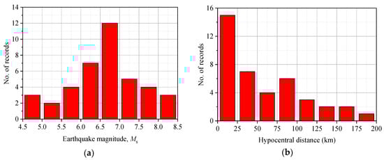
Figure 11.
Distribution of selected ground motion records versus (a) earthquake magnitude and (b) hypocentral distance.
3.3. Ground Motion Propagation for Deep Cover Soft Deposit
Using the typical Shanghai deep cover soft deposit and the ground motion records selected above, a nonlinear ground motion propagation analysis of the deposit was conducted, and computed ground surface acceleration time histories were obtained. These time histories were used as the input for studying seismic-induced energy spectra of an SDOF element on the deep cover soft deposit in the next step. Due to space limitations, a typical bedrock ground motion record (e.g., Chi-Chi, Taiwan-TAP077) and corresponding computed time history record were used, as shown in Figure 12. It is obvious that the deep cover soft deposit behaves as a filter when bedrock ground motions are transmitted through it.
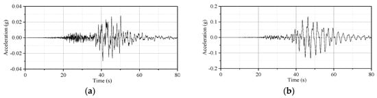
Figure 12.
Comparison of (a) the bedrock ground motion record and (b) the computed ground surface acceleration time history.
To highlight the use of ground motion propagation, normalized acceleration response spectra (with a 0.05 damping ratio) were calculated for the 40 bedrock ground motion records and computed ground surface acceleration time histories in Figure 13, where the results of TAP077 are shown as an example by a thicker line to clarify the effect of ground motion propagation. The following conclusions can be made: (1) The deep cover soft deposit makes the long-period component of the ground motion become dominant. Correspondingly, the low-frequency component of the ground motion is amplified and the high-frequency component is filtered out. (2) Compared with the input ground motion records at the bedrock, the predominant period of the computed ground surface acceleration time histories moves toward the long-period direction. The average predominant period of the 40 motion records was 0.30 s and of the 40 computed time histories was 0.87 s. Therefore, propagation of ground motion should be complemented by energy balance analysis when considering deep cover soft deposits.
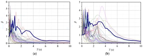
Figure 13.
Acceleration response spectra of (a) bedrock ground motion records and (b) computed ground surface acceleration time histories.
4. Energy Spectra for Damped and Inerter-Based Structures
Once the computed ground surface acceleration time histories were obtained by the nonlinear ground motion propagation for bedrock excitation, the energy spectra, including input and dissipation energy spectra, contributed by the primary SDOF element and the controlled system were obtained for the SDOF element and the inerter-based structure. Dealing with the ground motions, including different amplitudes and durations, the area of seismic-induced energy spectra [23] was employed to normalize energy responses. By means of the value, the energy spectra were normalized with respect to their area. We let denote the energy spectra ratios, representing the ratio of seismic-induced energy (per unit mass) to the area of total input energy , and this can be written as follows:
where the subscript represents , , and , denoting the input energy, dissipated energy of the primary SDOF element, and dissipated energy of the dashpot, respectively.
4.1. Energy Spectrum for Damped SDOF Element
Considering a series of SDOF elements with an inherent damping ratio where , a single dashpot where and the damping coefficient of the primary SDOF element is the same, and an undamped period varying from 0.02 s to 10 s, the normalized energy spectra can be calculated by Equations (13) and (17) for input energy () dissipated energy of the primary SDOF element (), and dissipated energy of the single dashpot (), shown in Figure 14, where the results of TAP077 are shown as an example by a thicker line. The subscript 0 refers to the condition of an SDOF element with a single dashpot.
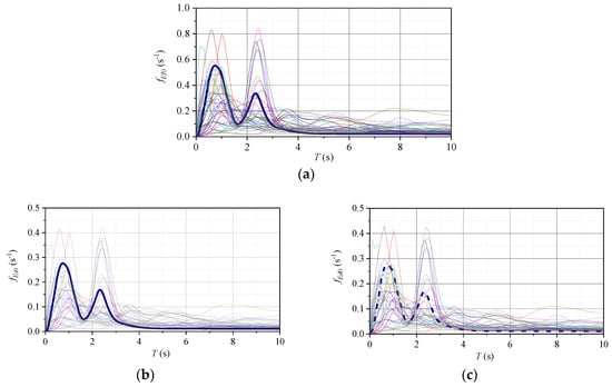
Figure 14.
Normalized seismic-induced energy spectra of SDOF element connected to a single dashpot. (a) Input energy spectra of SDOF element connected to a single dashpot. (b) Dissipated energy spectra of primary SDOF element. (c) Dissipated energy spectra of single dashpot.
As seen in Figure 14, the normalized curves of the energy spectra, including , , and , can be divided into three parts: ascending in the short period, where the spectral values increase with the period; plateau in the moderate period, where the spectral values fluctuate at some value; and descending in the long period, where the spectral values decline with the period. In addition, the normalized dissipated energy spectra of the primary SDOF element and single dashpot are approximately half of the input energy spectra . Note that the contributions of energy dissipation are the same for the SDOF element and the dashpot when their damping coefficients are the same.
Inspired by the results obtained in Figure 14, a model was adopted to approximate the energy spectra consisting of three regions: linear variation in the short periods, a constant region in the moderate periods, and a decreasing curve in the long periods. The three-region model can summarize the statistical characteristics of the seismic-induced energy spectrum. To provide an average result, the mean and mean plus one standard deviation (SD) curves of the normalized seismic-induced input energy spectra were calculated, shown in Figure 15. The mean plus one SD curve was used as a representative curve and the following equations were introduced to characterize the fitted three-region seismic input energy spectrum [23,56]:
where a is the normalized spectral ordinate, corresponding to the lower considered period, 0.02 s (); is the spectral value of the plateau of the energy spectrum; and denote the start and end periods of the plateau of the energy spectrum, respectively; and is the parameter governing the velocity of decay in the descending part of the energy spectrum.
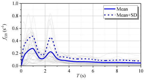
Figure 15.
Mean and mean plus one standard deviation (SD) curves of normalized seismic-induced input energy spectra of SDOF element connected to a single dashpot.
The least squares method was applied to the energy spectrum representative curve [56], thus:
where is the representative value and is the fitted value of the seismic-induced input energy spectrum of the SDOF element with a single dashpot. The fitted input spectrum is shown in Figure 16 and the corresponding parameters are given in Table 5. As illustrated in Table 5, the energy responses of structures with a long period () were large and located in the plateau. Consistent with the results from Section 3.3, the deep cover soft deposit causes a larger response for long-period structures, and this should be quantitatively considered.
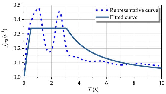
Figure 16.
Representative and fitted curves for seismic-induced input energy spectrum of SDOF element connected to a single dashpot.
Table 5.
Parameters for fitted elastic seismic-induced input energy spectrum.
4.2. Energy Spectrum for Inerter-Based Structure
In terms of the energy spectrum analysis for the inerter-based structure, a typical TVMD in Figure 4 was considered to suppress the oscillating vibration of the SDOF element. The key parameters of the TVMD were considered, including the inertance-to-mass ratio = 0.05, 0.10, and 0.25; the nominal damping ratio ; and the stiffness ratio . For a fair comparison, the damping coefficient of the TVMD was deliberately set to be the same as that of the single dashpot and primary SDOF element. Applying this TVMD to the primary SDOF elements considered in Section 4.1, normalized energy spectra were obtained for the input energy (), primary SDOF element (), and dashpot of the TVMD () under excitation of 40 computed ground surface acceleration time history responses, as shown in Figure 17.
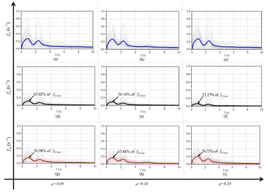
Figure 17.
Seismic-induced energy spectra of SDOF element connected to the TVMD.
After that, the mean curves of , , and were obtained and are given as solid blue, black, and red lines, respectively, in Figure 17. Comparing the input energy spectra in Figure 17a–c to the SDOF element connected to a dashpot in Figure 15, the input energies of the SDOF element connected to the TVMD and the single dashpot are the same, basically representing the same burden of energy dissipation. The fitted input energy in Figure 16 can be directly used for the SDOF-TVMD system. Faced with this, as evident from Figure 17g–i, with an increased inertance-to-mass ratio , the energy dissipated by the dashpot of the TVMD (characterized by ) increases rapidly, and it dissipates via the primary SDOF element (characterized by ), as shown in Figure 17d–f, where the decrease is dramatic.
Quantitatively, we let , , and denote the maximum values of , , and , respectively. It was shown that when , 0.10, and 0.25, the percentages are 43.02%, 36.16%, and 23.27% of respectively, whereas for they are 56.98%, 63.84%, and 76.73% of , respectively. To make this clear, the ratio of was calculated to be 1.33, 1.78, and 3.30 for , 0.10, and 0.25, respectively. Compared with the single dashpot with the same damping coefficient (), the TVMD exhibits improved ability and efficiency for energy dissipation (corresponding to > 50%), which is called the energy dissipation enhancement effect in this study. More importantly, a larger inertance-to-mass ratio is beneficial for this. According to the present study, the inerter of the TVMD amplifies the dashpot deformation and makes it larger than the entire deformation of the TVMD, which lays the foundation for improved energy dissipation. The energy spectrum analysis in this study explicitly reveals the energy mechanism and characteristics of a TVMD for the first time.
4.3. Optimal Design and Design Cases
Inspired by the revealed energy working basis of the inerter system, an optimal energy dissipation enhancement-based design principle is developed herein. As explained for Figure 17, from the energy perspective, the advantageous feature of the TVMD is the enhanced efficiency and ability of the dashpot to conduct energy dissipation. The pursuit of enhanced energy dissipation can potentially utilize the co-working mechanism of the inerter, the tuning spring, and the dashpot. For a structure with a predetermined damping ratio and oscillating period, the ratio of to , denoting the contribution of the dashpot and the value of the primary structure for energy dissipation, respectively, is selected as the optimization objective for maximization. The performance demand design principle is widely accepted as the orientation to guide structural design, which involves achieving stated performance objectives for structures when they are subjected to a stated intensity level of excitation [20,57,58]. Considering structural displacement as a key measurement, a target displacement control effect is considered as a constraint condition in the design problem. In summary, the proposed optimal energy dissipation enhancement-based design problem can be expressed in mathematical form:
where is the ratio of the root mean square of the displacement of the SDOF-TVMD system to that of the uncontrolled SDOF element. Considering that the maximum displacement is also a very important design parameter of the controlled system, this ratio can also be used in Equation (20) for optimal design. This optimization problem can be solved by the constrained nonlinear multivariable function fmincon compiled in MATLAB (MathWorks, Natick, MA, USA) [59].
Note that during the calculation of and for the optimal design, the computed ground surface acceleration time histories are suggested as the excitation, especially the ground motions, whose values closely match the fitted input spectrum in Figure 16. An illustrative case was used to introduce the implementation of the proposed optimal design strategy. An SDOF element with an undamped oscillating period of 1.0 s was considered, where was prespecified as 0.50. Taking the ground motion of TAP077 as an example, which matches Figure 16, substituting into Equation (20), the TVMD parameters can be optimized numerically and summarized as , , and .
To illustrate the advantages of the TVMD against the single dashpot and the uncontrolled SDOF element intuitively, the displacement and acceleration response results under the excitation of TAP077 and CHY102 are given in Figure 18, where the SDOF element controlled by a single dashpot with the same damping ratio of the TVMD is also analyzed. Inspecting Figure 18, including the root mean square and peak responses, it can be seen that the designed TVMD can provide the target displacement to the controlled system under different seismic excitations. The energy response results under different excitations are given in Figure 19. Comparing the single dashpot and TVMD, the designed TVMD shows increased energy dissipation ability (indicated by the black arrow), while the primary structure has a decreased energy dissipation burden (indicated by the red arrow). Quantitatively, the ratio of to is maximized as 2.09 and 2.10 for TAP077 and CHY102, respectively, which is consistent with the results of the optimization design. In addition, the same operation is conducted for the 40 studied signals, of which the average results are summarized. The ratios of root mean square displacement and acceleration of the SDOF-TVMD system to that of the uncontrolled SDOF element are 0.515 and 0.512, respectively. The average result of is 2.08. The statistical results above demonstrate that the optimal design method proposed in this study can be well applied to the parameter determination of the TVMD with sufficient utilization of its energy-based benefit.
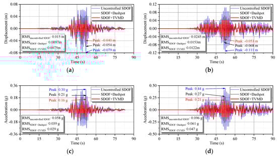
Figure 18.
Displacement and acceleration response results of designed SDOF elements. (a) Displacement under excitation of TAP077. (b) Displacement under excitation of CHY102. (c) Acceleration under excitation of TAP077. (d) Acceleration under excitation of CHY102.
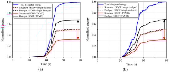
Figure 19.
Energy response results of designed SDOF elements. (a) Energy responses under the excitation of TAP077. (b) Energy responses under the excitation of CHY102.
5. Conclusions
Considering the underlying soil, this study performed a systematic energy spectrum analysis for the SDOF element controlled by TVMD in order to reveal the energy dissipation enhancement mechanism of the TVMD compared with a single dashpot. Taking advantage of the revealed energy benefit, an optimal energy dissipation enhancement-based design strategy was proposed for optimization of the TVMD. The main conclusions of this study are as follows:
- The developed energy spectrum analysis framework effectively quantifies the degree of the energy dissipation enhancement effect of the TVMD. Compared with a single dashpot with the same damping coefficient, the TVMD exhibits improved efficiency for energy dissipation, with less energy required for the primary structure to dissipate.
- Based on the revealed energy characteristic of the inerter system, the optimal design strategy can guarantee the target demand of displacement control, which optimizes the efficiency and quantity of the TVMD for energy dissipation, reducing the energy dissipation burden on the primary structure.
- Taking the effect of the underlying soil into consideration, especially deep cover soft deposits, a fitted seismic input energy spectrum is provided for the inerter-based structure, which facilitates the optimal energy-based design of the TVMD.
- For an inerter-based structure on a deep cover soft deposit, nonlinear ground motion propagation should be quantitatively considered for energy analysis and optimal design. After considering the underlying soil, the input energy and dissipated energy responses are dominant and large for long-period inerter-based structures (), owing to the effects of the underlying soil.
The objective of this study was to develop an energy spectrum analysis framework for an SDOF-TVMD system by considering the soil underneath the inerter-based structure. In future studies, the nonlinear behavior of the interaction between soil and inerter-based structures should be incorporated into the numerical and experimental analysis for more complex structures, and its effect in the corresponding optimal design should be investigated.
Author Contributions
Conceptualization: Q.C.; methodology: Q.C., Y.W., and Z.Z.; software: Y.W. and Z.Z.; validation: Q.C., Z.Z., and Y.W.; formal analysis: Z.Z. and Y.W.; investigation: Q.C., Y.W., and Z.Z.; data curation: Y.W. and Z.Z.; writing—original draft preparation: Q.C., Y.W., and Z.Z.; writing—review and editing: Q.C., Y.W., Z.Z. All authors have read and agreed to the published version of the manuscript.
Funding
This study was supported by the National Natural Science Foundation of China (grant number 51778489), the National Science and Technology Pillar Program of China (grant no. 2015BAK17B04), and the Basic Research Project of State Key Laboratory of Ministry of Science and Technology (grant number SLDRCE19A-02).
Conflicts of Interest
The authors declare no conflict of interest.
References
- Takewaki, I.; Murakami, S.; Yoshitomi, S.; Tsuji, M. Fundamental mechanism of earthquake response reduction in building structures with inertial dampers. Struct. Control Health Monit. 2012, 19, 590–608. [Google Scholar] [CrossRef]
- Zhang, R.F.; Zhao, Z.P.; Dai, K. Seismic response mitigation of a wind turbine tower using a tuned parallel inerter mass system. Eng. Struct. 2019, 180, 29–39. [Google Scholar] [CrossRef]
- Masri, S.F.; Caffrey, J.P. Transient response of a sdof system with an inerter to nonstationary stochastic excitation. J. Appl. Mech. Trans. Asme 2017, 84, 041005. [Google Scholar] [CrossRef]
- Jiang, Y.Y.; Zhao, Z.P.; Zhang, R.F.; De Domenico, D.; Pan, C. Optimal design based on analytical solution for storage tank with inerter isolation system. Soil Dyn. Earthq. Eng. 2020, 129, 105924. [Google Scholar] [CrossRef]
- Barredo, E.; Blanco, A.; Colín, J.; Penagos, V.M.; Abúndez, A.; Vela, L.G.; Meza, V.; Cruz, R.H.; Mayén, J. Closed-form solutions for the optimal design of inerter-based dynamic vibration absorbers. Int. J. Mech. Sci. 2018, 144, 41–53. [Google Scholar] [CrossRef]
- Chen, Q.J.; Zhao, Z.P.; Zhang, R.F.; Pan, C. Impact of soil–structure interaction on structures with inerter system. J. Sound Vib. 2018, 433, 1–15. [Google Scholar] [CrossRef]
- Zhang, R.F.; Zhao, Z.P.; Pan, C. Influence of mechanical layout of inerter systems on seismic mitigation of storage tanks. Soil Dyn. Earthq. Eng. 2018, 114, 639–649. [Google Scholar] [CrossRef]
- Ikago, K.; Saito, K.; Inoue, N. Seismic control of single-degree-of-freedom structure using tuned viscous mass damper. Earthq. Eng. Struct. Dyn. 2012, 41, 453–474. [Google Scholar] [CrossRef]
- Arakaki, T.; Kuroda, H.; Arima, F.; Inoue, Y.; Baba, K. Development of seismic devices applied to ball screw: Part 1 Basic performance test of RD-series. J. Archit. Build. Sci. 1999, 5, 239–244. [Google Scholar] [CrossRef]
- De Domenico, D.; Deastra, P.; Ricciardi, G.; Sims, N.D.; Wagg, D.J. Novel fluid inerter based tuned mass dampers for optimised structural control of base-isolated buildings. J. Frankl. Inst. 2019, 356, 7626–7649. [Google Scholar] [CrossRef]
- Kawamata, S. Development of a Vibration Control System of Structures by Means of Mass Pumps; Institute of Industrial Science, University of Tokyo: Tokyo, Japan, 1973. [Google Scholar]
- Smith, M.C. Synthesis of mechanical networks: The inerter. IEEE Trans. Autom. Control 2002, 47, 1648–1662. [Google Scholar] [CrossRef]
- Gonzalez-Buelga, A.; Clare, L.R.; Neild, S.A.; Jiang, J.Z.; Inman, D.J. An electromagnetic inerter-based vibration suppression device. Smart Mater. Struct. 2015, 24, 055015. [Google Scholar] [CrossRef]
- Lazar, I.F.; Neild, S.A.; Wagg, D.J. Using an inerter-based device for structural vibration suppression. Earthq. Eng. Struct. Dyn. 2014, 43, 1129–1147. [Google Scholar] [CrossRef]
- Zhao, Z.P.; Zhang, R.F.; Lu, Z. A particle inerter system for structural seismic response mitigation. J. Frankl. Inst. 2019, 356, 7669–7688. [Google Scholar] [CrossRef]
- Zhao, Z.P.; Zhang, R.F.; Jiang, Y.Y.; Pan, C. A tuned liquid inerter system for vibration control. Int. J. Mech. Sci. 2019, 164, 105171. [Google Scholar] [CrossRef]
- Chen, Q.J.; Zhao, Z.P.; Xia, Y.Y.; Pan, C.; Luo, H.; Zhang, R.F. Comfort based floor design employing tuned inerter mass system. J. Sound Vib. 2019, 458, 143–157. [Google Scholar] [CrossRef]
- Javidialesaadi, A.; Wierschem, N.E. Optimal design of rotational inertial double tuned mass dampers under random excitation. Eng. Struct. 2018, 165, 412–421. [Google Scholar] [CrossRef]
- Zhang, R.F.; Zhao, Z.P.; Pan, C.; Ikago, K.; Xue, S.T. Damping enhancement principle of inerter system. Struct. Control Health Monit. 2020. [Google Scholar] [CrossRef]
- Pan, C.; Zhang, R.F.; Luo, H.; Li, C.; Shen, H. Demand-based optimal design of oscillator with parallel-layout viscous inerter damper. Struct. Control Health Monit. 2018, 25, e2051. [Google Scholar] [CrossRef]
- Zhao, Z.P.; Zhang, R.F.; Jiang, Y.Y.; Pan, C. Seismic response mitigation of structures with a friction pendulum inerter system. Eng. Struct. 2019, 193, 110–120. [Google Scholar] [CrossRef]
- Zhao, Z.P.; Chen, Q.J.; Zhang, R.F.; Pan, C.; Jiang, Y.Y. Optimal design of an inerter isolation system considering the soil condition. Eng. Struct. 2019, 196, 109324. [Google Scholar] [CrossRef]
- Decanini, L.D.; Mollaioli, F. Formulation of elastic earthquake input energy spectra. Earthq. Eng. Struct. Dyn. 1998, 27, 1503–1522. [Google Scholar] [CrossRef]
- Bagheri, B.; Oh, S.H. Seismic design of coupled shear wall building linked by hysteretic dampers using energy based seismic design. Int. J. Steel Struct. 2018, 18, 225–253. [Google Scholar] [CrossRef]
- Benavent-Climent, A.; Lopez-Almansa, F.; Bravo-Gonzalez, D.A. Design energy input spectra for moderate-to-high seismicity regions based on Colombian earthquakes. Soil Dyn. Earthq. Eng. 2010, 30, 1129–1148. [Google Scholar] [CrossRef]
- Reggio, A.; De Angelis, M. Optimal energy-based seismic design of non-conventional Tuned Mass Damper (TMD) implemented via inter-story isolation. Earthq. Eng. Struct. Dyn. 2015, 44, 1623–1642. [Google Scholar] [CrossRef]
- Tan, J.; Jiang, J.; Liu, M.; Feng, Q.; Zhang, P.; Ho, S.C.M. Implementation of shape memory alloy sponge as energy dissipating material on pounding tuned mass damper: An experimental investigation. Appl. Sci. Basel 2019, 9, 1079. [Google Scholar] [CrossRef]
- Benavent-Climent, A.; Escobedo, A.; Donaire-Avila, J.; Oliver-Saiz, E.; Ramirez-Marquez, A.L. Assessment of expected damage on buildings subjected to Lorca earthquake through an energy-based seismic index method and nonlinear dynamic response analyses. Bull. Earthq. Eng. 2014, 12, 2049–2073. [Google Scholar] [CrossRef]
- Benavent-Climent, A.; Mota-Paez, S. Earthquake retrofitting of R/C frames with soft first story using hysteretic dampers: Energy-based design method and evaluation. Eng. Struct. 2017, 137, 19–32. [Google Scholar] [CrossRef]
- Benavent-Climent, A. An energy-based method for seismic retrofit of existing frames using hysteretic dampers. Soil Dyn. Earthq. Eng. 2011, 31, 1385–1396. [Google Scholar] [CrossRef]
- Alici, F.S.; Sucuoglu, H. Elastic and inelastic near-fault input energy spectra. Earthq. Spectra 2018, 34, 611–637. [Google Scholar] [CrossRef]
- Gullu, A.; Yuksel, E.; Yalcin, C.; Dindar, A.A.; Ozkaynak, H.; Buyukozturk, O. An improved input energy spectrum verified by the shake table tests. Earthq. Eng. Struct. Dyn. 2019, 48, 27–45. [Google Scholar] [CrossRef]
- Schnabel, P.B.; Lysmer, J.; Seed, H.B. SHAKE: A Computer Program for Earthquake Response Analysis of Horizontally Layered Sites, Report No. UCB/EERC-72/12; Earthquake Engineering Research Center, University of California: Berkeley, CA, USA, 1972. [Google Scholar]
- Wang, Z.L.; Dafalias, Y.F.; Shen, C.K. Bounding surface hypoplasticity model for sand. J. Eng. Mech. 1990, 116, 983–1001. [Google Scholar] [CrossRef]
- Martin, P.P.; Seed, H.B. One-dimensional dynamic ground response analyses. J. Geotech. Eng. Div. Asce 1982, 108, 935–952. [Google Scholar] [CrossRef]
- Srbulov, M. Geotechnical Earthquake Engineering: Simplified Analyses with Case Studies and Examples; Springer Science & Business Media: Berlin/Heidelberg, Germany, 2008. [Google Scholar]
- Jabary, R.; Madabhushi, S. Structure-soil-structure interaction effects on structures retrofitted with tuned mass dampers. Soil Dyn. Earthq. Eng. 2017, 100, 301–315. [Google Scholar] [CrossRef]
- Wu, J.; Chen, G.; Lou, M. Seismic effectiveness of tuned mass dampers considering soil–structure interaction. Earthq. Eng. Struct. Dyn. 1999, 28, 1219–1233. [Google Scholar] [CrossRef]
- Hashash, Y.M.A.; Park, D. Non-linear one-dimensional seismic ground motion propagation in the Mississippi embayment. Eng. Geol. 2001, 62, 185–206. [Google Scholar] [CrossRef]
- Ge, Q.; Xiong, F.; Xie, L.; Chen, J.; Yu, M. Dynamic interaction of soil-Structure cluster. Soil Dyn. Earthq. Eng. 2019, 123, 16–30. [Google Scholar] [CrossRef]
- Chong, S.H. Soil dynamic constitutive model for characterizing the nonlinear-hysteretic response. Appl. Sci. Basel 2017, 7, 1110. [Google Scholar] [CrossRef]
- Uang, C.M.; Bertero, V.V. Evaluation of seismic energy in structures. Earthq. Eng. Struct. Dyn. 1990, 19, 77–90. [Google Scholar] [CrossRef]
- Chapman, M.C. On the use of elastic input energy for seismic hazard analysis. Earthq. Spectra 1999, 15, 607–635. [Google Scholar] [CrossRef]
- Ordaz, M.; Huerta, B.; Reinoso, E. Exact computation of input-energy spectra from Fourier amplitude spectra. Earthq. Eng. Struct. Dyn. 2003, 32, 597–605. [Google Scholar] [CrossRef]
- Wang, Y.C.; Chen, Q.J. Parametric fitting of soft soil sites’ Davidenkov model based on PSO algorithm and its application. J. Vib. Shock 2019, 38, 8–16. [Google Scholar]
- Yang, L.D.; Wang, G.B.; Liu, Q.J.; Lei, G. A study on the dynamic properties of soft soil in shanghai. In Proceedings of the Soil and Rock Behavior and Modeling, Shanghai, China, 6 June 2006; pp. 466–473. [Google Scholar]
- Lanzo, G.; Vucetic, M. Effect of soil plasticity on damping ratio at small cyclic strains. Soils Found. 1999, 39, 131–141. [Google Scholar] [CrossRef]
- Clough, R.W.; Penzien, J. Dymnics of Structures; McCraw-Hill: New York, NY, USA, 1975. [Google Scholar]
- ABAQUS. Theory and Analysis User’s Manual Version 6.12; Dassault Systems SIMULIA Corp: Providence, RI, USA, 2012. [Google Scholar]
- Finn, W.D.; Lee, K.W.; Martin, G.R. An effective stress model for liquefaction. Am. Soc. Civ. Eng. J. Geotech. Eng. Div. 1977, 103, 517–533. [Google Scholar]
- Carlton, B.; Tokimatsu, K. Comparison of equivalent linear and nonlinear site response analysis results and model to estimate maximum shear strain. Earthq. Spectra 2016, 32, 1867–1887. [Google Scholar] [CrossRef]
- Garini, E.; Gazetas, G.; Ziotopoulou, K. Inelastic soil amplification in three sites during the Tokachi-oki M-JMA 8.0 earthquake. Soil Dyn. Earthq. Eng. 2018, 110, 300–317. [Google Scholar] [CrossRef]
- Huang, Y.; Ye, W.; Chen, Z. Seismic response analysis of the deep saturated soil deposits in Shanghai. Environ. Geol. 2009, 56, 1163–1169. [Google Scholar] [CrossRef]
- University of California. Berkeley. PEER NGA-West2 Ground Motion Database. Available online: http://ngawest2.berkeley.edu/ (accessed on 8 January 2020).
- Trifunac, M.D.; Brady, A.G. Study on duration of strong earthquake ground motion. Bull. Seismol. Soc. Am. 1975, 65, 581–626. [Google Scholar]
- Zhou, Y.; Song, G.; Huang, S.; Wu, H. Input energy spectra for self-centering SDOF systems. Soil Dyn. Earthq. Eng. 2019, 121, 293–305. [Google Scholar] [CrossRef]
- Kim, J.; Kim, S. Performance-based seismic design of staggered truss frames with friction dampers. Thin Walled Struct. 2017, 111, 197–209. [Google Scholar] [CrossRef]
- Nabid, N.; Hajirasouliha, I.; Petkovski, M. Adaptive low computational cost optimisation method for performance-based seismic design of friction dampers. Eng. Struct. 2019, 198, 109549. [Google Scholar] [CrossRef]
- MATLAB Documentation Center, Optimization Toolbox, Constrained Optimization, Fmincon. Available online: http://www.mathworks.com/help/optim/ug/fmincon.html (accessed on 8 January 2020).

© 2020 by the authors. Licensee MDPI, Basel, Switzerland. This article is an open access article distributed under the terms and conditions of the Creative Commons Attribution (CC BY) license (http://creativecommons.org/licenses/by/4.0/).