A Novel Architecture to Classify Histopathology Images Using Convolutional Neural Networks


Abstract
1. Introduction
- We propose a novel CNN architecture that can classify histopathology images with high accuracy.
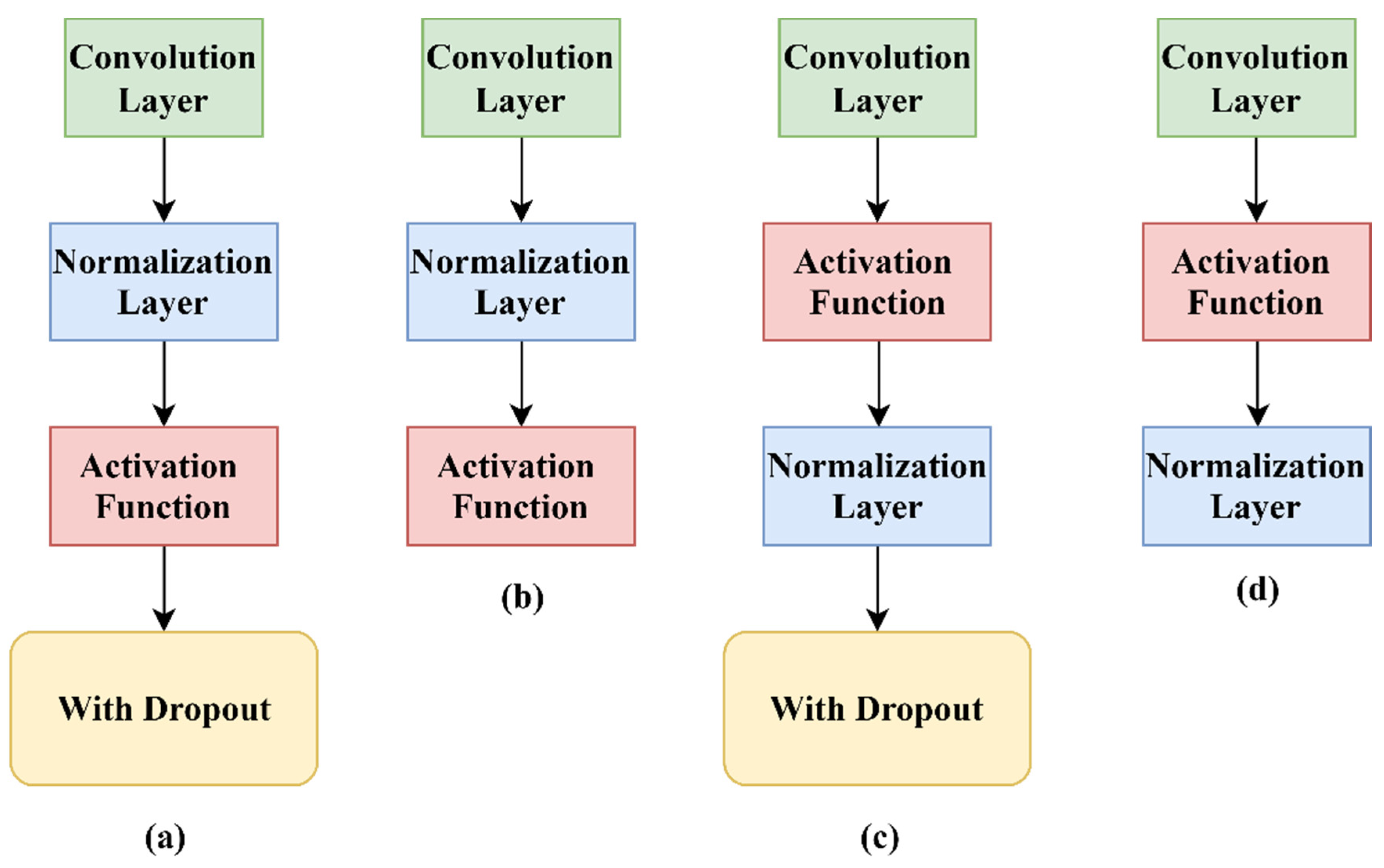
- We investigate the impact of dropout layers and the impact of the location of the normalization layer.
- We test six activation functions to study their impact on the proposed architecture, rather than choosing the de-facto ReLU activation function.
- We study the impact of two different optimizers on the CNN performance.
- We consider four popular state-of-the-art CNNs to compare the performance of our model. These CNNs were trained on the PatchCamelyon dataset. These results can be used by researchers instead of training these models again from scratch, which can take hours (if not days), especially in the lack of computational power.
2. Literature Review
2.1. VGG Architectures
2.2. InceptionV3 Architecture
2.3. ResNet Architecture
3. Methodology
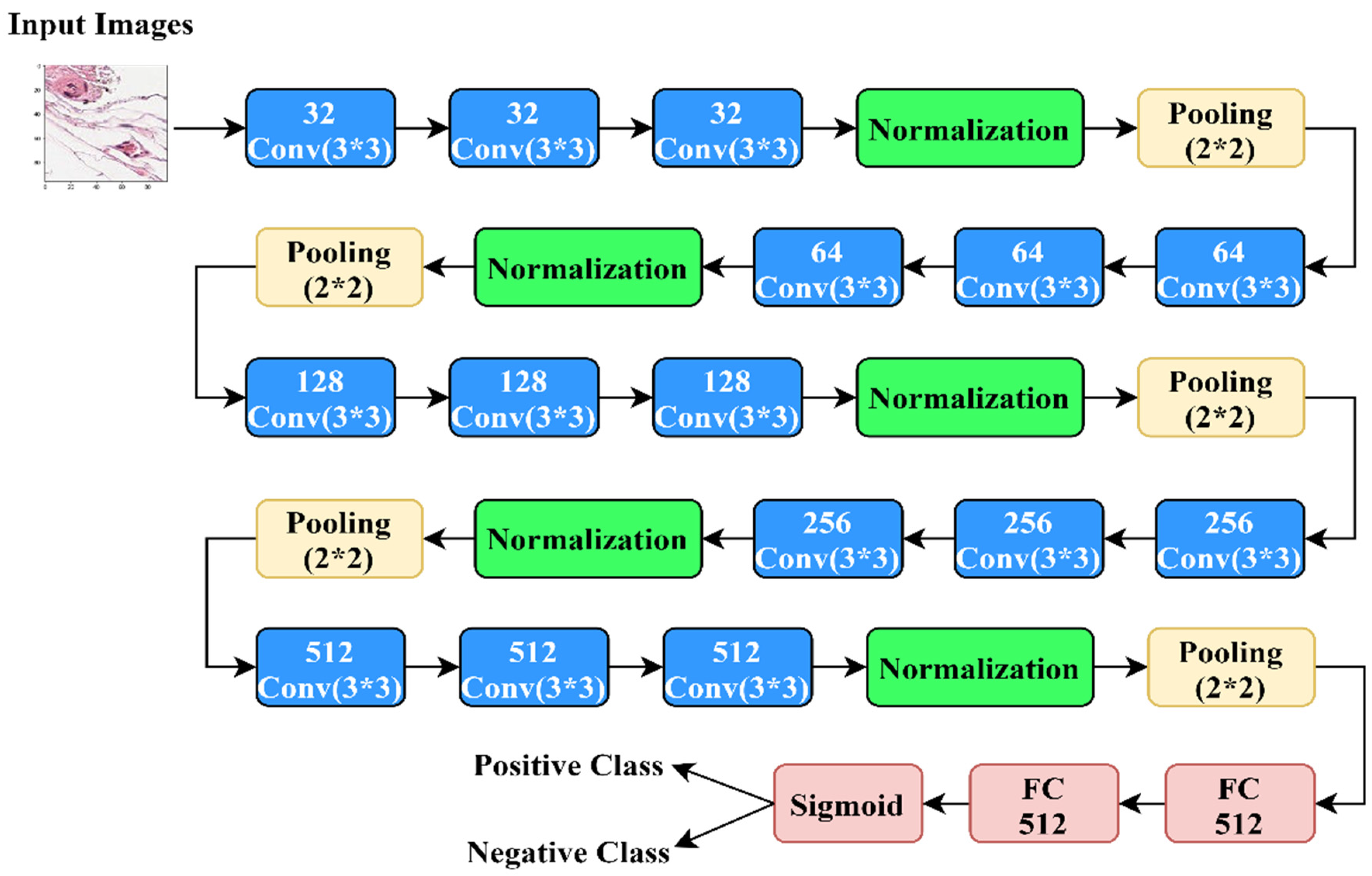
3.1. Proposed Architecture
3.2. Dataset
4. Results
4.1. Experimental Setup
4.2. Results
4.2.1. The Results of Different Activation Functions
4.2.2. The Results of Different Designs
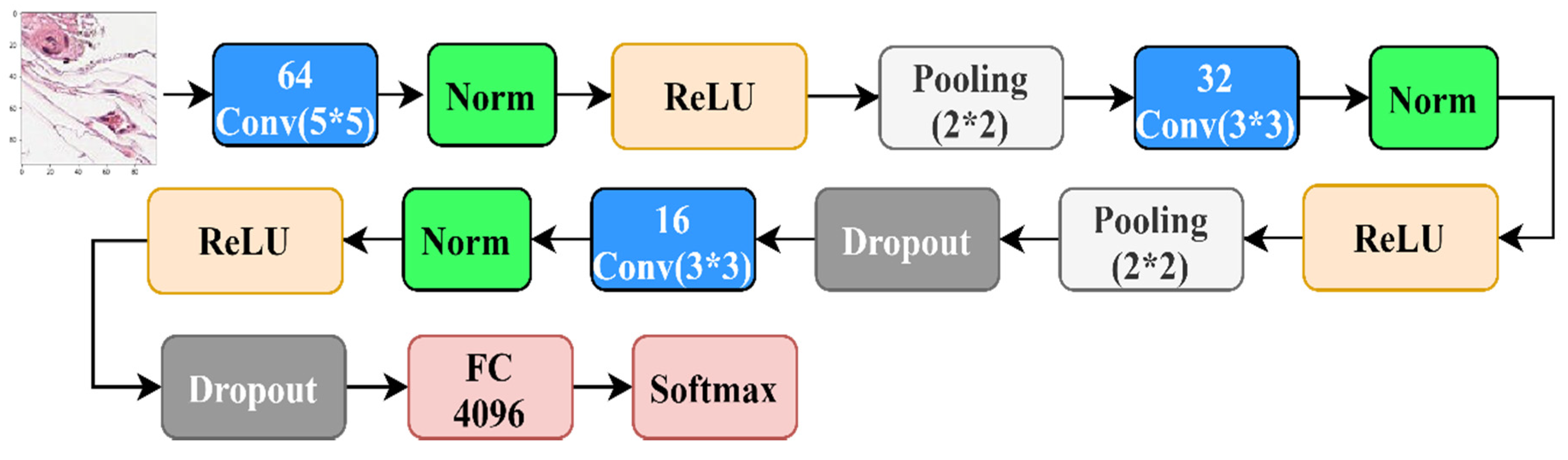
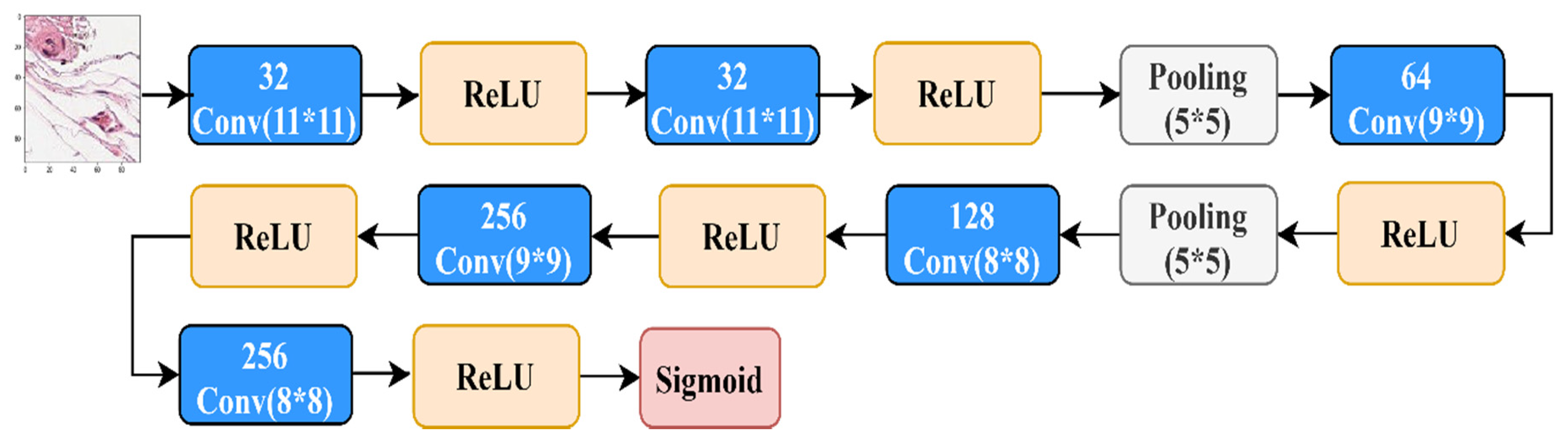
4.2.3. The Results over Benchmark CNN Architectures
4.2.4. The Results of State-of-the-Art CNN Architectures
5. Discussion
5.1. Histopathology Images Importance And Challenges
5.2. The Presented Architecture Choice
5.3. The Effect of Different Activation Functions
5.4. The Effect of the Location of the Normalization Layer and the Dropout Layer
5.5. Comparison between Different Benchmark CNN
5.6. Comparison between Different State-of-the-Art CNN
6. Conclusions
Author Contributions
Funding
Acknowledgments
Conflicts of Interest
References
- Siegel, R.L.; Miller, K.D.; Jemal, A. Cancer statistics. CA. Cancer J. Clin. 2020, 70, 7–30. [Google Scholar] [CrossRef] [PubMed]
- World Health Organization. Cancer 2018. Available online: https://www.who.int/news-room/fact-sheets/detail/cancer (accessed on 12 February 2020).
- He, L.; Long, L.; Antani, S.; Thoma, G. Histology image analysis for carcinoma detection and grading. Comput. Methods Programs Biomed. 2012, 107, 538–556. [Google Scholar] [CrossRef] [PubMed]
- Robbins, P.; Pinder, S.; de Klerk, N.; Dawkins, H.; Harvey, J.; Sterrett, G.; Ellis, I.; Elston, C. Histological grading of breast carcinomas: A study of interobserver agreement. Hum. Pathol. 1995, 26, 873–879. [Google Scholar] [CrossRef]
- Metter, D.; Colgan, T.; Leung, S.; Timmons, C. Trends in the US and Canadian Pathologist Workforces From 2007 to 2017. JAMA Netw. Open 2019, 2, e194337. [Google Scholar] [CrossRef]
- LeCun, Y.; Boser, B.; Denker, J.S.; Henderson, D.; Howard, R.E.; Hubbard, W.; Jackel, L.D. Backpropagation Applied to Handwritten Zip Code Recognition. Neural Comput. 1989, 1, 541–551. [Google Scholar] [CrossRef]
- Krizhevsky, A.; Sutskever, I.; Hinton, G.E. ImageNet Classification with Deep Convolutional Neural Networks. Neural Inf. Process. Syst. 2012, 25, 1097–1105. [Google Scholar] [CrossRef]
- Russakovsky, O.; Deng, J.; Su, H.; Krause, J.; Satheesh, S.; Ma, S.; Huang, Z.; Karpathy, A.; Khosla, A.; Bernstein, M.; et al. ImageNet Large Scale Visual Recognition Challenge. Int. J. Comput. Vis. 2015, 115, 211–252. [Google Scholar] [CrossRef]
- Luo, H.; Yang, Y.; Tong, B.; Wu, F.; Fan, B. Traffic Sign Recognition Using a Multi-Task Convolutional Neural Network. IEEE Trans. Intell. Transp. Syst. 2018, 19, 1100–1111. [Google Scholar] [CrossRef]
- Sermanet, P.; LeCun, Y. Traffic sign recognition with multi-scale Convolutional Networks. In Proceedings of the 2011 International Joint Conference on Neural Networks, San Jose, CA, USA, 31 July–5 August 2011; pp. 2809–2813. [Google Scholar]
- Kim, Y. Convolutional Neural Networks for Sentence Classification. In Proceedings of the 2014 Conference on Empirical Methods in Natural Language Processing (EMNLP), Doha, Qatar, 25–29 October 2014; pp. 1746–1751. [Google Scholar]
- Zhang, X.; Zhao, J.; LeCun, Y. Character-Level Convolutional Networks for Text Classification. In Proceedings of the 28th International Conference on Neural Information Processing Systems, Montreal, QC, Canada, 8–13 December 2015; Volume 1, pp. 649–657. [Google Scholar]
- Abdel-Hamid, O.; Mohamed, A.; Jiang, H.; Deng, L.; Penn, G.; Yu, D. Convolutional Neural Networks for Speech Recognition. IEEE/ACM Trans. Audio Speech Lang. Process. 2014, 22, 1533–1545. [Google Scholar] [CrossRef]
- Abdel-Hamid, O.; Mohamed, A.; Jiang, H.; Penn, G. Applying Convolutional Neural Networks concepts to hybrid NN-HMM model for speech recognition. In Proceedings of the 2012 IEEE International Conference on Acoustics, Speech and Signal Processing (ICASSP), Kyoto, Japan, 25–30 March 2012; pp. 4277–4280. [Google Scholar]
- Gehring, J.; Auli, M.; Grangier, D.; Yarats, D.; Dauphin, Y. Convolutional Sequence to Sequence Learning. In Proceedings of the 34th International Conference on Machine Learning (ICML 2017), Sydney, Australia, 6–11 August 2017. [Google Scholar]
- Gehring, J.; Auli, M.; Grangier, D.; Dauphin, Y. A Convolutional Encoder Model for Neural Machine Translation. arXiv Prepr. 2017, arXiv:1611.02344. [Google Scholar]
- Veeling, B.S.; Linmans, J.; Winkens, J.; Cohen, T.; Welling, M. Rotation Equivariant CNNs for Digital Pathology BT–Medical Image Computing and Computer Assisted Intervention–MICCAI 2018; Springer Cham: Granada, Spain, 2018; pp. 210–218. [Google Scholar]
- Ehteshami Bejnordi, B.; Veta, M.; Johannes van Diest, P.; van Ginneken, B.; Karssemeijer, N.; Litjens, G.; van der Laak, J.A.W.M.; the CAMELYON16 Consortium, Hermsen, M. Diagnostic Assessment of Deep Learning Algorithms for Detection of Lymph Node Metastases in Women With Breast Cancer. JAMA 2017, 318, 2199–2210. [Google Scholar] [CrossRef] [PubMed]
- Lecun, Y.; Bottou, L.; Bengio, Y.; Haffner, P. Gradient-based learning applied to document recognition. Proc. IEEE 1998, 86, 2278–2324. [Google Scholar] [CrossRef]
- Nguyen, P.T.; Nguyen, T.T.; Nguyen, N.C.; Le, T.T. Multiclass Breast Cancer Classification Using Convolutional Neural Network. In Proceedings of the 2019 International Symposium on Electrical and Electronics Engineering (ISEE), Ho Chi Minh, Vietnam, 10–12 October 2019; pp. 130–134. [Google Scholar]
- Bayramoglu, N.; Kannala, J.; Heikkila, J. Deep learning for magnification independent breast cancer histopathology image classification. In Proceedings of the 2016 23rd International Conference on Pattern Recognition (ICPR), Cancun, Mexico, 4–8 December 2016. [Google Scholar]
- Arjmand, A.; Angelis, C.T.; Tzallas, A.T.; Tsipouras, M.G.; Glavas, E.; Forlano, R.; Manousou, P.; Giannakeas, N. Deep Learning in Liver Biopsies using Convolutional Neural Networks. In Proceedings of the 2019 42nd International Conference on Telecommunications and Signal Processing (TSP), Budapest, Hungary, 1–3 July 2019; pp. 496–499. [Google Scholar]
- Sirinukunwattana, K.; Raza, S.E.A.; Tsang, Y.; Snead, D.R.J.; Cree, I.A.; Rajpoot, N.M. Locality Sensitive Deep Learning for Detection and Classification of Nuclei in Routine Colon Cancer Histology Images. IEEE Trans. Med. Imaging 2016, 35, 1196–1206. [Google Scholar] [CrossRef] [PubMed]
- Lai, Z.; Deng, H. Medical Image Classification Based on Deep Features Extracted by Deep Model and Statistic Feature Fusion with Multilayer Perceptron. Comput. Intell. Neurosci. 2018, 2018, 1–13. [Google Scholar] [CrossRef] [PubMed]
- Basha, S.H.S.; Ghosh, S.; Babu, K.; Dubey, S.; Pulabaigari, V.; Mukherjee, S. RCCNet: An Efficient Convolutional Neural Network for Histological Routine Colon Cancer Nuclei Classification. In Proceedings of the 2018 15th International Conference on Control, Automation, Robotics and Vision (ICARCV), Singapore, 18–21 November 2018. [Google Scholar]
- Simonyan, K.; Zisserman, A. Very Deep Convolutional Networks for Large-Scale Image Recognition. arXiv 2014, arXiv:1409.1556. [Google Scholar]
- Szegedy, C.; Vanhoucke, V.; Ioffe, S.; Shlens, J.; Wojna, Z.B. Rethinking the Inception Architecture for Computer Vision. In Proceedings of the IEEE Conference on Computer Vision and Pattern Recognition (CVPR), Las Vegas, NV, USA, 26 June–1 July 2016; pp. 2818–2826. [Google Scholar]
- He, K.; Zhang, X.; Ren, S.; Sun, J. Deep Residual Learning for Image Recognition. In Proceedings of the IEEE Conference on Computer Vision and Pattern Recognition (CVPR), Las Vegas, NV, USA, 27–30 June 2016; pp. 770–778. [Google Scholar]
- Nair, V.; Hinton, G.E. Rectified linear units improve restricted boltzmann machines. In Proceedings of the 27th international conference on machine learning (ICML-10), Haifa, Israel, 21–24 June 2010. [Google Scholar]
- Maas, A.L.; Hannun, A.Y.; Ng, A.Y. Rectifier nonlinearities improve neural network acoustic models. In Proceedings of ICML 2013, Atlanta, GA, USA, 16–21 June 2013. [Google Scholar]
- Clevert, D.-A.; Unterthiner, T.; Hochreiter, S. Fast and Accurate Deep Network Learning by Exponential Linear Units (ELUs). arXiv Prepr. 2016, arXiv:1511.07289. [Google Scholar]
- Klambauer, G.; Unterthiner, T.; Mayr, A.; Hochreiter, S. Self-Normalizing Neural Networks. In Proceedings of the Advances in Neural Information Processing Systems 2017, Long Beach, CA, USA, 4–9 December 2017; pp. 971–980. [Google Scholar]
- Kingma, D.; Ba, J. Adam: A Method for Stochastic Optimization. Int. Conf. Learn. Represent. 2014, arXiv:1412.6980. [Google Scholar]
- Ruder, S. An overview of gradient descent optimization algorithms. arXiv Prepr. 2016, arXiv:1609.04747. [Google Scholar]
- Shorten, C.; Khoshgoftaar, T.M. A survey on image data augmentation for deep learning. J. Big Data 2019, 6, 60. [Google Scholar] [CrossRef]
- Chollet, F. Keras; GitHub: San Francisco, CA, USA, 2015. [Google Scholar]
- Abadi, M.; Agarwal, A.; Barham, P.; Brevdo, E.; Chen, Z.; Citro, C.; Corrada, G.S.; Davis, A.; Dean, J.; Devin, M.; et al. TensorFlow: Large-Scale Machine Learning on Heterogeneous Distributed Systems. arXiv 2015, arXiv:1603.04467. [Google Scholar]
- Ioffe, S.; Szegedy, C. Batch normalization: Accelerating deep network training by reducing internal covariate shift. arXiv Prepr. 2015, arXiv:1502.03167. [Google Scholar]


| Authors | Main Contribution | Number of Classes | Metric | Test Set Performance |
|---|---|---|---|---|
| Nguyen et al. [20] |
| 8 | Accuracy | 73.68% |
| Bayramoglu et al. [21] |
| 2 for the malignant/not malignant task 8 for the magnification task | Accuracy | 83.25% 80.10% |
| Arjmand et al. [22] |
| 2 | Accuracy | 95% |
| Sirinukunwattana et al. [23] |
| 4 | F1 Score | 0.692 (This is the combined performance on nucleus detection and classification) |
| Lai et al. [24] |
| 2 | Accuracy | 90.1% and 90.2% on two benchmark medical image datasets |
| Basha et al. [25] |
| 4 | F1 Score | 0.7887 |
| Conv Layers | FC layers | Dropout Layers | Normalization Layers | Activation Function | Pooling Layers | |
|---|---|---|---|---|---|---|
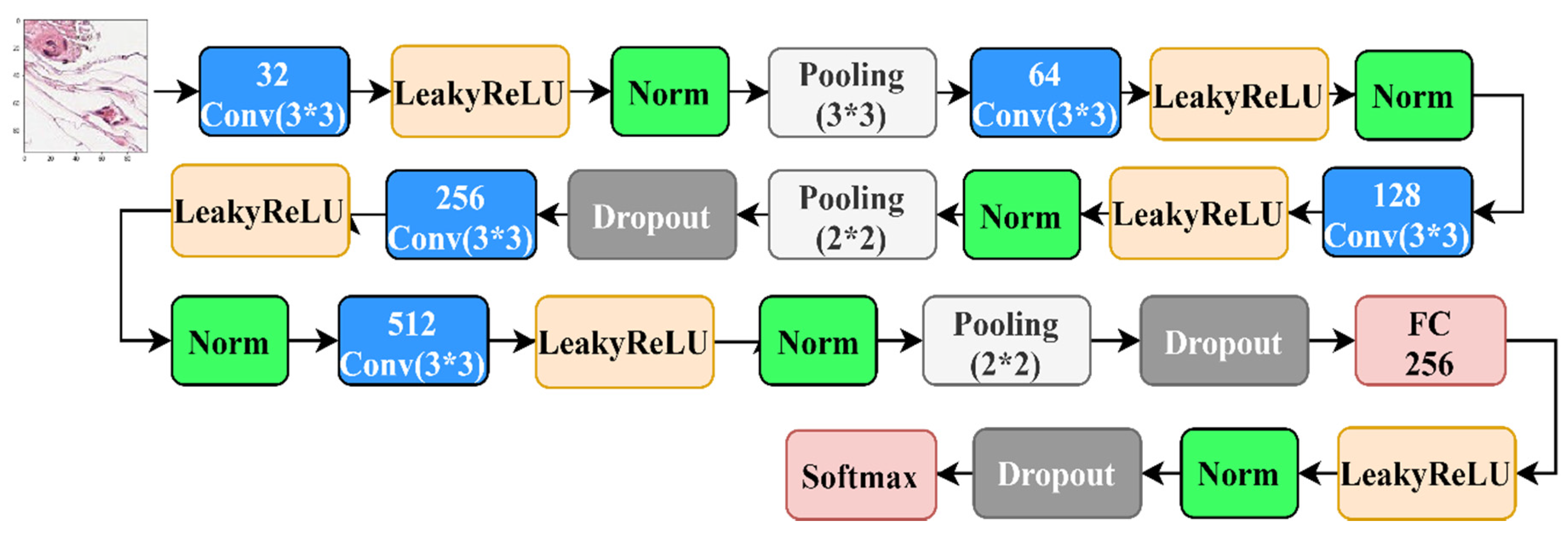
| Nguyen et al. [20] | 5 | 1 | 3 | 6 | LeakyReLU | 3 |
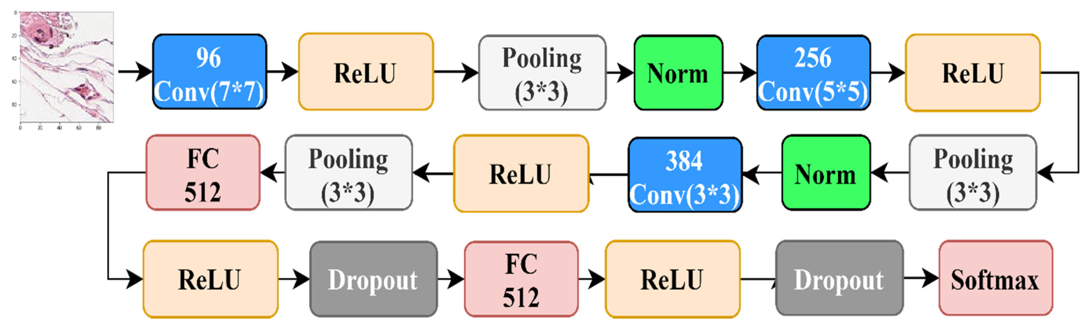
| Bayramoglu et al. [21] | 3 | 2 | 2 | 2 | ReLU | 3 |
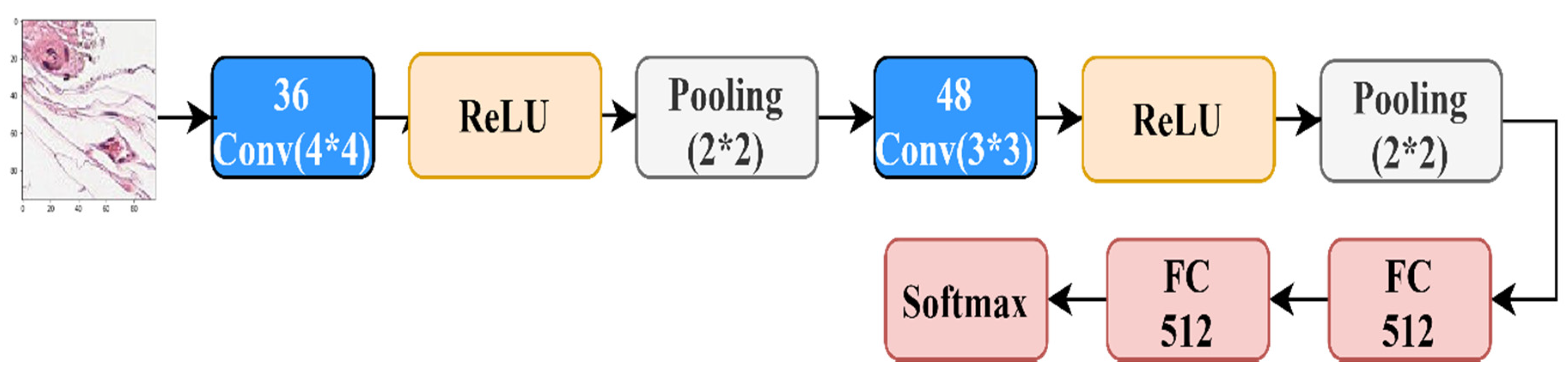
| Arjmand et al. [22] | 3 | 1 | 2 | 3 | ReLU | 2 |
| Sirinukunwattana et al. [23] | 2 | 2 | 0 | 0 | ReLU | 2 |
| Lai et al. [24] | 6 | 0 | 0 | 0 | ReLU | 2 |
| Basha et al. [25] | 4 | 2 | 2 | 6 | ReLU | 2 |
| ReLU | LeakyReLU | ELU | SELU | Sigmoid | Tanh | |
|---|---|---|---|---|---|---|
| Adam | 87.68% | 87.37% | 93.66% | 92.73% | 84.03% | 91.70% |
| RMSprop | 85.01% | 83.02% | 92.99% | 88.43% | 84.49% | 92.00% |
| Tanh | ReLU | LeakyReLU | ELU | SELU | |
|---|---|---|---|---|---|
| H1 | 91.70% | 87.68% | 87.37% | 93.66% | 92.73% |
| H2 | 92.96% | 85.45% | 87.17% | 91.76% | 92.82% |
| H3 | 94.39% | 91.78% | 89.96% | 94.40% | 90.16% |
| H4 | 95.46% | 89.33% | 89.11% | 93.85% | 92.71% |
| Tanh | ReLU | LeakyReLU | ELU | SELU | |
|---|---|---|---|---|---|
| H1 | 92.00% | 85.01% | 83.02% | 92.99% | 88.43% |
| H2 | 94.09% | 89.77% | 90.37% | 87.62% | 94.25% |
| H3 | 93.35% | 88.40% | 90.38% | 92.26% | 93.86% |
| H4 | 93.43% | 87.70% | 90.11% | 94.86% | 91.58% |
| RMSProp | Adam | |
|---|---|---|
| Our Model | 92.99% | 93.66% |
| VGG16 | 84.22% | 89.53% |
| VGG19 | 89.08% | 90.64% |
| InceptionV3 | 82.66% | 82.47% |
| ResNet | 85.24% | 81.21% |
| RMSProp | Adam | |
|---|---|---|
| Our Model | 94.86% | 95.46% |
| VGG16 | 89.33% | 91.00% |
| VGG19 | 89.24% | 89.20% |
| InceptionV3 | 87.15% | 85.88% |
| ResNet | 78.01% | 83.52% |
© 2020 by the authors. Licensee MDPI, Basel, Switzerland. This article is an open access article distributed under the terms and conditions of the Creative Commons Attribution (CC BY) license (http://creativecommons.org/licenses/by/4.0/).
Share and Cite
Kandel, I.; Castelli, M. A Novel Architecture to Classify Histopathology Images Using Convolutional Neural Networks. Appl. Sci. 2020, 10, 2929. https://doi.org/10.3390/app10082929
Kandel I, Castelli M. A Novel Architecture to Classify Histopathology Images Using Convolutional Neural Networks. Applied Sciences. 2020; 10(8):2929. https://doi.org/10.3390/app10082929
Chicago/Turabian StyleKandel, Ibrahem, and Mauro Castelli. 2020. "A Novel Architecture to Classify Histopathology Images Using Convolutional Neural Networks" Applied Sciences 10, no. 8: 2929. https://doi.org/10.3390/app10082929
APA StyleKandel, I., & Castelli, M. (2020). A Novel Architecture to Classify Histopathology Images Using Convolutional Neural Networks. Applied Sciences, 10(8), 2929. https://doi.org/10.3390/app10082929