A Novel Method of Seismic Signal Detection Using Waveform Features

Abstract

The detection of seismic signals is vital in seismic data processing and analysis. Many algorithms have been proposed to resolve this issue, such as the ratio of short-term and long-term power averages (STA/LTA), F detector, Generalize F, and etc. However, the detection performance will be affected by the noise signals severely. In this paper, we propose a novel seismic signal detection method based on the historical waveform features to improve the seismic signals detection performance and reduce the affection from the noise signals. We use the historical events location information in a specific area and waveform features information to build the joint probability model. For the new signal from this area, we can determine whether it is the seismic signal according to the value of the joint probability. The waveform features used to construct the model include the average spectral energy on a specific frequency band, the energy of the component obtained by decomposing the signal through empirical mode decomposition (EMD), and the peak and the ratio of STA/LTA trace. We use the Gaussian process (GP) to build each feature model and finally get a multi-features joint probability model. The historical events location information is used as the kernel of the GP, and the historical waveform features are used to train the hyperparameters of GP. The beamforming data of the seismic array KSRS of International Monitoring System are used to train and test the model. The testing results show the effectiveness of the proposed method.

1. Introduction

Seismic arrays have been widely used in the area of seismic monitoring and nuclear test monitoring. Seismic arrays are composed of multiple sensors located in a certain range, and the signal-to-noise ratio of far-field signals can be effectively improved by means of delay and sum beamforming. The detection capability of seismic signals can be improved [1,2]. Compared with three-component stations, seismic arrays can provide more accurate estimates of signal azimuth and slowness through techniques such as FK analysis [3,4]. Scholars have proposed various data processing and analysis methods for seismic arrays, which are powerful tools to improve detection capabilities and reduce manual workload. Impulsive noise signals usually come from the instrument, human-made, and nature. Noise signals are often mixed in seismic signals, which causes false detection of events and inaccurate parameter calculations. How to effectively detect seismic signals and accurately identify seismic phases from noise signals is one of the challenges we have to face.

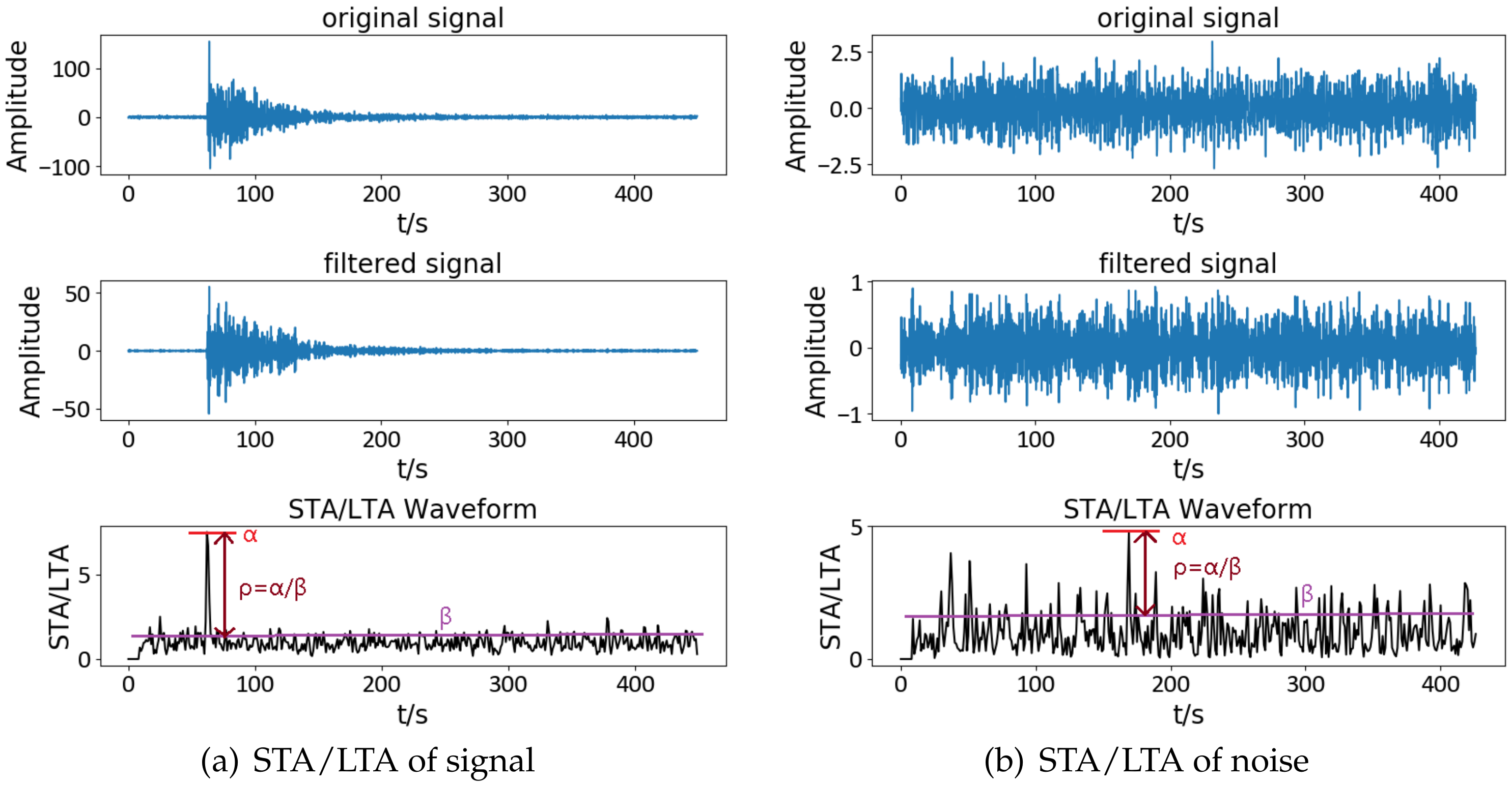
Over the past decades, the traditional STA/LTA method [5,6,7] has been used to pick up seismic signals. It reflects the instantaneous change in signal energy by calculating the ratio of the short-term and long-term average of data. It has been widely used in many real-time detection systems, such as Earthquake Early Warning (EEW), seismic data processing software Seiscomp3, CTBTO International Data Centre waveform data processing software IDCR3, Geotool, and so on. The limitation of STA/LTA is that it is sensitive to the time-varying background noise [7], which increases the probability of small-signal misdetection. So it is not suitable for lower SNR signals [8]. For the signals with SNR between 1.5 dB and 3 dB, researchers have used the denoising method based on discrete wavelet transform (DWT) to improve the performance of the STA/LTA algorithm [9]. Besides, the setting of the threshold and the selection of the characteristic function also can affect the detection sensitivity [10]. For local seismic signals, there are some high-frequency components, which are stronger than that in teleseismic signals. Besides the amplitude detection, we can use the frequency component information to detect the local seismic signals. However, for the teleseismic signals, the high-frequency components are weak due to the long propagation distance. It is more suitable for teleseismic signals to use multiple regional stations or arrays to enhance the detection reliability [11]. Utilizing cross-correlation techniques [12], we can efficiently detect the teleseimic signals. So the accuracy of receiving arrival time can be developed. Beamforming [13,14] also can increase the SNR and the detection performance by delaying and summing the records of substations of the same array using signal correlation and simultaneously eliminate the effects of non-coherent noise. Blandford [15] firstly proposed to apply F detection to study strongly coherent teleseismic signals, but F detection has higher requirements for seismic signals and noise. For example, the seismic signals are stationary and Gaussian, while noise is uncorrelated. Generalized F (GF) detector can process small-aperture array signals and has no special demands for noise, which makes up for the shortcomings of F detection. However, GF is limited to other factors influencing the proportion of false alarms [16], such as the prior SNR, the selection of signal model parameter $t^{*}$ and requiring a usable noise correlation model for each array. Additionally, the signals across the array should not vary greatly. The matched signal detector [17] performs correlation processing between the detection signal and the template waveform. The higher the similarity between the two waveforms, the larger the correlation function value is. Template matching solves the problem of weak seismic signals detection, which [18,19,20,21] advances the detection threshold with the coherent seismic signals. However, the generality of this method is limited by the dependence on source assumptions, and this method requires a huge number of historical earthquakes to form a template library. It will not be applied to some areas where earthquakes have never happened [20,22,23,24]. Machine learning (ML) and neural network have been widely used in seismology, especially for detecting and identifying P phase, S phase, and noise. With the rapid growth of seismic data, machine learning and deep learning plays a significant role in processing vast amounts of seismic data [25,26,27,28]. However, these algorithms often require a lot of work to deal with massive data in the previous stage to prepare data sets, and the precision of classification depends on the trained model [29,30,31].

In this paper, we propose a novel method based on location information and waveform features to detect the seismic signal. A signal model combining multiple features was built. The waveform features are the spectral energy average about the specific frequency band of the signal, the energy of the signal component decomposing by empirical mode decomposition, the peak and the ratio of STA/LTA trace. The Gaussian Process(GP) was used to build the model distribution. GP [32,33,34,35] is a popular method for Bayesian non-linear non-parametric regression and classification in machine learning. It is a collection of real-valued functions and any finite number of random variables have a joint Gaussian distribution. Three years of CTBTO International Monitoring System (IMS) KSRS array data were used to train the model.

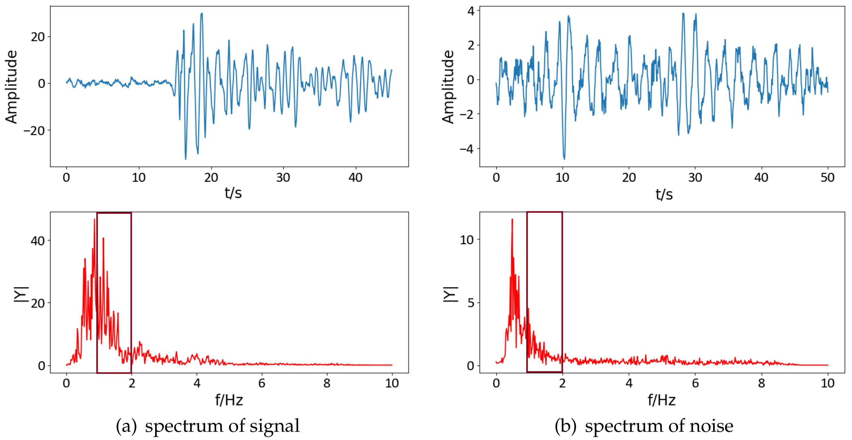
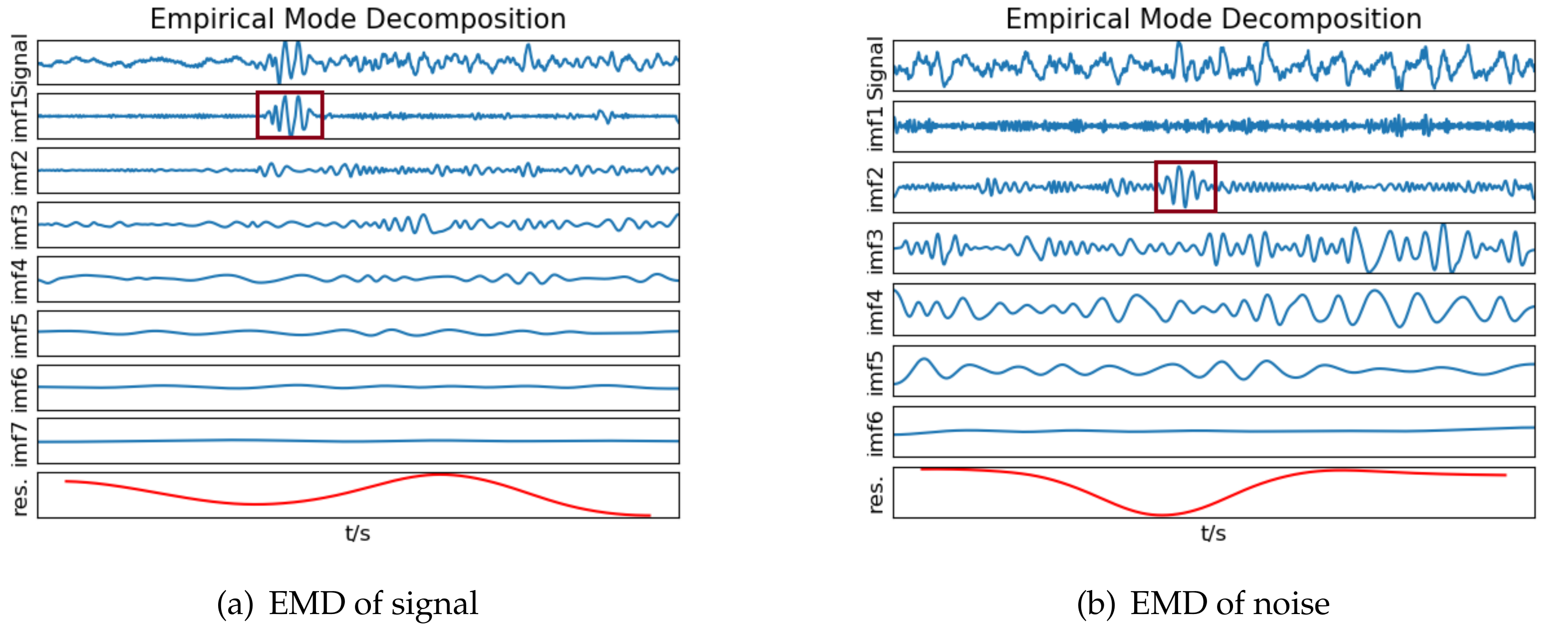
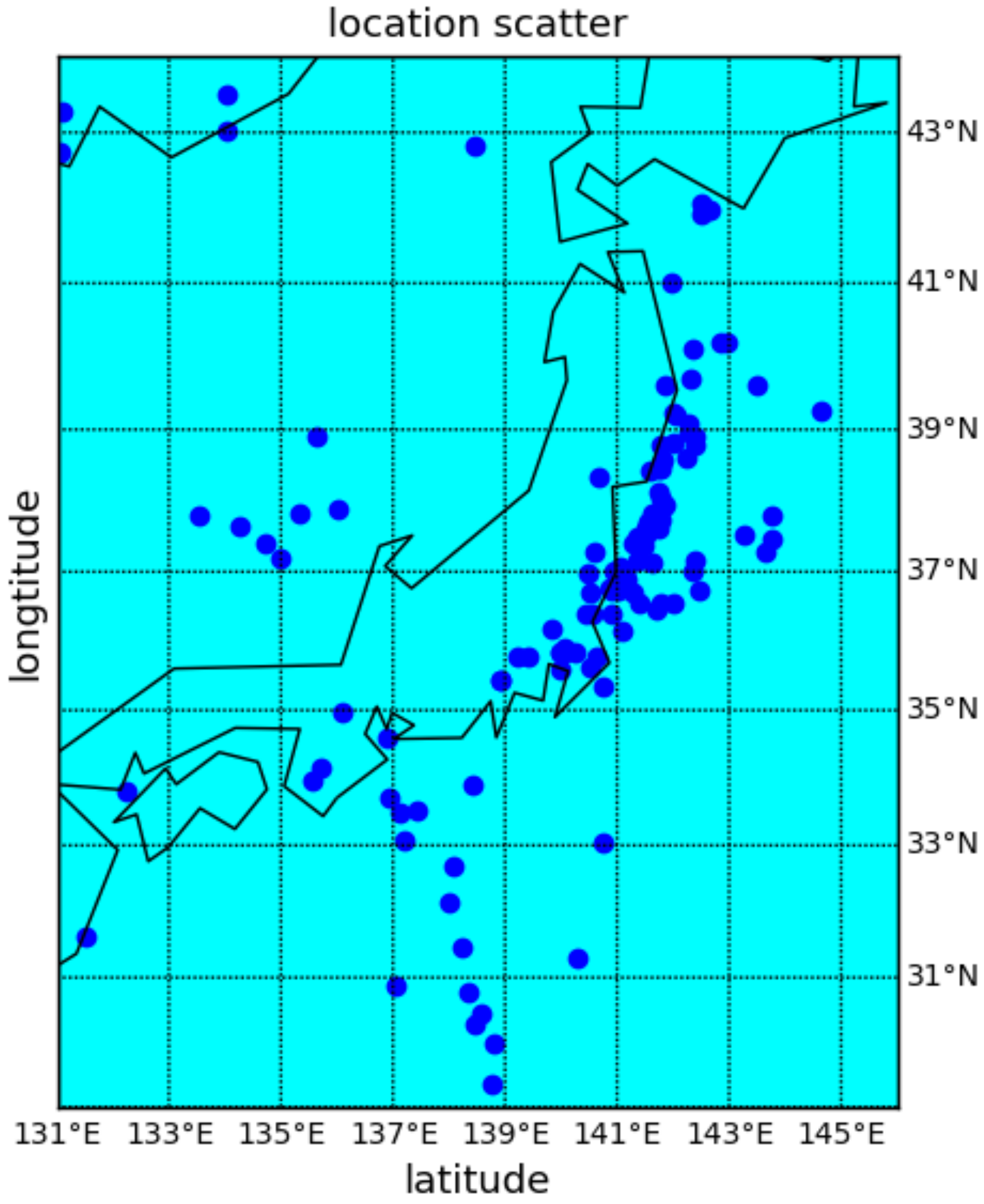
Seismic signal detection is constituted of four main steps in this paper. Firstly, data preparation is an essential step in the whole process, and it is used for selecting some observed seismic events for researching. Secondly, the feature extraction step obtains a lot of valuable information on original signals. By analyzing the signal, we choose some helpful features in the seismic signal detection, such as the peak and ratio of the STA/LTA trace, the average value of energy in a specific frequency band, and the energy value after empirical mode decomposition (EMD), which are independent of each other and introduced in detail later. Thirdly, the single-feature model is constructed by location and waveform information. Each feature obeys the Gaussian distribution generated from GP. Lastly, we calculate the posterior probability of the joint features to predict the possibility that new signal is a seismic signal. During the process, the optimal hyperparameters of GP are obtained by maximizing the marginal likelihood function L($\theta$) [32].

In summary, the innovations and contributions of this work have several points:

• Focusing on a specific region, waveform features that are suitable for seismic signal detection are chosen and extracted, such as the envelop features of STA/LTA trace and frequency-domain energy features of the signal.
• The Gaussian process with event location information in a specific region as a kernel function is used to build the signal features model. The seismic detection is achieved using joint features probability model.

In the following sections, first of all, a brief introduction of GP is introduced. Next, waveform features used in this paper are described in detail, and a joint multi-features probability model is constructed. Then the implementation of seismic signal detection method proposed in this paper is elaborated, including data preparation, feature extraction, model training, and etc. Finally, we analyze and discuss the results.

2. Theory and Methods

2.1. Gaussian Process

In general, the Gaussian process (GP) regression is a powerful tool, which generates distribution over functions applied to non-parametric regression [36]. In Gaussian process regression, we assume the output y of a function f at input x can be written as

$$y=f\left(x\right)+ϵ.$$

(1)

In Equation (1), the observation signal y is composed of the signal term $f\left(x\right)$ and the noise term $ϵ$, with $ϵ\sim (0,\sigma {}_n^2)$ being independent and identically distributed.

The distribution of function $f\left(x\right)$ comes from a Gaussian process, which is defined by a mean and a covariance function.

$$f\left(x\right)\sim \mathcal{GP}(m\left(x\right),k(x,x^{\prime }))$$

(2)

$$m\left(x\right)=\mathbb{E}\left[f\right(x\left)\right]$$

(3)

$$k(x,x^{\prime })=\mathbb{E}\left[(f\left(x\right)-m\left(x\right))(f\left(x^{\prime }\right)-m\left(x^{\prime }\right))\right],$$

(4)

where the mean function $m\left(x\right)$ reflects the expected function value at input x. The covariance function $k(x,x{}^{\prime })$ shows the correlation between input x and test point $x^{\prime }$. The function k is commonly called the kernel of the Gaussian process [37].

Given an observation data set $D=(X,y)$ of n elements, where $(X,y)$ is a pair of input-output data, the output $f_{*}$ is predicted by the conditional distribution $p\left(f\right|D)$ at the test input $x_{*}$. According to the definition, the joint multivariate distribution of previous observations y and function values $f_{*}$ can be expressed as

$$\left[\begin{array}{c}y\\ f_{*}\end{array}\right]\sim \mathrm{N}\left(\left[\begin{array}{cc}K\left(X,X\right)+{\sigma }_n^{2}I& K\left(X,X_{*}\right)\\ K(X_{*},X)& K\left(X_{*},X_{*}\right)\end{array}\right]\right),$$

(5)

where $K(X,X)$, $K(X,X_{*})$, $K(X_{*},X)$ and $K(X_{*},X_{*})$ are $n\times n$ covariance matrices. These are similarly evaluated from n training points and n test points. When there is only one test point, we can calculate the covariance vector between a test point and n training points in same way, indicated as $K(X,X)$, $K(X,x_{*})$, $K(x_{*},X)$ and $K(x_{*},x_{*})$.

We can derive the conditional distribution function $p\left(f\right|D)$, which is the crucial predictive equation for Gaussian process regression,

$$p(f_{*};X,X_{*})=\mathrm{N}(\overline{f_{*}},{\sum }_{*}^f)$$

(6)

where the mean function is

$$\overline{f_{*}}=K(X_{*},X){[K(X,X)+{\sigma }_n^{2}I]}^{-1}y$$

(7)

and the covariance function is

$${\sum }_{*}^f=k(X_{*},X_{*})-K(X_{*},X){[K(X,X)+{\sigma }_n^{2}I]}^{-1}K(X,X_{*}).$$

(8)

For the single test point, we can rewrite the mean function in the following way,

$$m\left(x_{*}\right)=\sum _{i=1}^n{w}_{i}k(x_i,x_{*})$$

(9)

$$w={[K\left(X,X\right)+{\sigma }_n^{2}I]}^{-1}y,$$

(10)

where X is the observed data set, $x_i$ is the element in X, $w_i$ is the weight computed by the Equation (10). So we can make a new prediction of new point $x_{*}$ by weighted sum. The output $y_{*}$ is associated with the data set X. The kernel shows the similarity between the prediction point $x_{*}$ and input $x_i$ of the observation set X.

The covariance function is also called the kernel. The choice of an appropriate kernel is based on assumptions such as smoothness and likely patterns to be expected in the data [36]. The marten kernel is chosen for the calculation of the Gaussian process, which is usually used in geography.

$$k_{\mathrm{Martern}}\left(r\right)={\sigma }_f^2\exp \left(\frac{\mathsf{\Gamma }(p+1)}{\mathsf{\Gamma }(2p+1)}\right)\sum _{i=0}^p\frac{(p+i)!}{i!(p-i)!}{\left(\frac{r\sqrt{8p+4}}{l}\right)}^{p-i}$$

(11)

in the Equation (11), p is an integer, and $p=v+\frac{1}{2}$. With the $p=1$, the above formula can be reduced to

$$k_{v=\frac{3}{2}}\left(r\right)={\sigma }_f^2\left(1+\frac{\sqrt{3r}}{l}\right)\exp \left(-\frac{\sqrt{3r}}{l}\right)$$

(12)

$$r(x,x^{\prime })=\sqrt{d_{earth}(lon,lat),(lo{n}^{\prime },la{t}^{\prime }){)}^2},$$

(13)

where r is the distance between the two points on the surface of the earth and related to the geographic location of longitude and latitude. This paper uses the Geographical spherical distance to calculate the earth’s surface distance. The correlation of two points depends on the distance between x and $x^{\prime }$. Therefore, the similarity between the near points is higher than the far points.

2.2. Optimizing Hyper-Parameters

The hyperparameters in the Equation (11) are the length-scale l, the signal variance ${\sigma }_f^2$, and the noise variance ${\sigma }_n^2$, which are unknown and need to be inferred from the observations. Obtaining the hyper-parameters is maximizing the marginal (log) likelihood through a optimization tool of gradient ascent. Using the training set $D=\left\{(X_i,y_i)\right|i=1,2,\dots ,n\}$ and the hyper-parameters vector $\theta$$(\theta =(l,{\sigma }_f^2,{\sigma }_n^2))$, the log marginal likelihood is

$$\begin{array}{cc}\hfill \mathrm{L}\left(\theta \right)& =\log p\left(y\right|X,\theta )\hfill \\ \hfill & =-\frac{1}{2}{y}^T{K}_y^{-1}y-\frac{1}{2}\log \left|K_y\right|-\frac{n}{2}\log 2\pi ,\hfill \end{array}$$

(14)

with $K_y=K(X,X)+{\sigma }_n^{2}I$. The equation is composed of three terms, denoting a fit penalizing measure. The term $-\frac{1}{2}{y}^T{K}_y^{-1}y$ shows degree of data-fit. The term $-\frac{1}{2}\log \left|K_y\right|$ is related to the kernel and observation inputs, displaying the complexity penalty. The term $-\frac{n}{2}\log 2\pi$ is a normalization constant.

The partial derivative of $\theta$ plays a vital role in seeking the optional value of gradient ascent, which is obtained by the Equation (14),

$$\begin{array}{cc}\hfill \frac{\partial }{\partial {\theta }_j}\log p\left(y\right|X,\theta )& =\frac{1}{2}{y}^T{K}_y^{-1}y-\frac{1}{2}\mathrm{tr}\left(K_y^{-1}\frac{\partial K_y}{\partial {\theta }_j}\right)\hfill \\ \hfill & =\frac{1}{2}\mathrm{tr}\left((w{w}^T-K_y^{-1})\frac{\partial K_y}{\partial {\theta }_j}\right).\hfill \end{array}$$

(15)

3. Signal Model

3.1. Waveform Features

Based on the statistics and observations about a series of seismic events, we analyze waveform features in the time domain and energy features in the frequency domain. We can identify some useful features to distinguish seismic signals and noise. These features include the amplitude $\alpha$ and the ratio $\rho$ of the STA/LTA trace of the seismic waveform, signal energy mean $\gamma$ in the same length time window near the arrival of the signal and the power $\lambda$ of the intrinsic mode function 1 (IMF1) after the waveform decomposed by EMD.

In Figure 1, we can see the seismic signal amplitude is higher than noise. Statistically, the mean value of the Gaussian distribution of seismic signals is higher than the mean of noise signals, as shown in

Table 1. Statistical distribution of each waveform feature.

Class	Signal Train Set		Signal Test Set		Noise Test Set
	Mean	Standard Deviation	Mean	Standard Deviation	Mean	Standard Deviation
$\alpha$	5.19	1.45	5.66	1.55	2.61	0.38
$\rho$	4.08	1.49	4.48	1.53	1.96	0.28
$\log$($\gamma$)	3.95	2.61	4.51	2.60	0.04	0.69
$\log$($\lambda$)	8.62	2.86	9.19	2.88	4.74	0.87

. So the probability of noise is usually smaller compared to the seismic signal obtained by the predictive distribution from the Gaussian process. Additionally, as shown in Figure 1, it can be seen that the noise has many visible fluctuations. The ratio value is the largest peak divided by the average of other spikes. The ratio of the signal is higher than the noise. In Figure 2, we can notice the difference between the spectrogram of the seismic signal and noise. The waveform energy average of the seismic signal is higher than the noise for 1–2 Hz, so the band energy average can be utilized as another feature to distinguish signals and noise. In addition, EMD can decompose the non-stationary non-linear signal into a series of various frequency sub-components, namely the IMF, reflecting many inherent information of the signal. In Figure 3, we can note that the signal is decomposed into a group of IMF components, arranged in descending order of frequency. After statistics, it was found that the main component containing most seismic signal energy was the IMF1 part. Then, we used the energy of IMF1 to distinguish seismic signals and noise.

3.2. Establish a Signal Model

After extracting the characteristics of historic seismic events, the next question is how to use these features to build a model. For each signal, the corresponding feature elements are available from the time domain and the frequency domain. Using the Gaussian process, we can obtain every feature distribution. We assume that all waveform features are independent. Then the joint probability model is as follows,

$$p\left(s_i\right|E)=p\left({\alpha }_i\right|E)p\left({\rho }_i\right|E)p\left(\log {\gamma }_i|E\right)p\left(\log {\lambda }_i|E\right).$$

(16)

In the Equation (16), $p\left(s_i\right|E)$ is the occurring probability value of a seismic signal in the specific area. We use $p(•|E)$ to denote the probability value for every feature. We adopt $\log (•)$ to indicate logarithmic normalization of data.

In the following, take the amplitude feature as an example to introduce the modeling process, and similarly for other features. For a specific phase of a particular array, by observing a large number of historical event waveforms, the observation can be expressed as the sum of an unknown function about the event origin $f_j^{\left(k\right)}\left(e\right)$ and a noise term $ϵ$ in Equation (17). Through the GP, the model of the amplitude characteristics is established as Equation (18),

$$f_{\alpha }=f\left(e_i\right)+ϵ$$

(17)

$$f_{{\alpha }_i}\sim GP({\mu }_{\alpha ,j}^k,k_{\alpha ,j}^k)$$

(18)

According to the Equation (18), the occurrence probability of the amplitude about a new observation signal $s_i$ can be predicted.

$$p\left({\alpha }_i\right|E)=\mathrm{N}(\overline{f_{*}}\left(E\right),{\sum }_{*}^f\left(E\right))$$

(19)

in the Equation (19), ${\overline{f}}_{*}$ is mean and ${\sum }_{*}^f$ is covariance of the test point computed separately by Equations (7) and (8).

4. Implementation

4.1. Data Preparation

We choose a specific area of Japan and adjacent seas where earthquakes occur more frequently and can provide a large number of historical events for study, guaranteeing the data used for the research are sufficient. Then, three years (from May 2011 to May 2014) of data from the KSRS station about 266 events are selected as the data set, and it is randomly divided into a training set and a test set. Furthermore, the same amount of impulsive noise data are chosen as part of the test set.

In this section, we select a specific region for studying how to detect the teleseismic P phase accurately. As depicted in Figure 4, the location and size of the region is longitude (29${}^{\circ }$ N∼44${}^{\circ }$ N) and latitude (131${}^{\circ }$ E∼146${}^{\circ }$ E). The reason for picking a specific region is the covariance function in the Gaussian process is related to the correlation of the signals, and the mean function is the linear combination of kernel functions about input points. If the selected region is too wide, the correlation of the signals will be weak. In supervised learning, the concept of similarity between data points is crucial. This is an underlying assumption that points close to the input x are likely to have similar target values, so training points close to the test points can provide information for prediction, see Equations (4)–(14).

To further explain the relationship between distance and correlation, we select three locations among the corner area of (33${}^{\circ }$ N∼38${}^{\circ }$ N) and (135${}^{\circ }$ E∼140${}^{\circ }$ E), which are (136${}^{\circ }$ E, 34${}^{\circ }$ N), (135.4${}^{\circ }$ E, 37${}^{\circ }$ N), and (139.6${}^{\circ }$ E, 36${}^{\circ }$ N). As shown in Figure 5, except for the blue line, the other three lines indicate three locations where the earthquake occur possibly. The vertical axis represents the locations of historical events. The horizontal axis shows the location correlation between the new predictive signal and observed seismic events. The larger the corresponding value on the vertical axis, the greater the possibility of a new seismic signal occur in this area. The blue line represents a location where an event has never occurred at (137${}^{\circ }$ E, 35${}^{\circ }$ N). As can be seen from the image, the covariance of the blue line is zero in all locations; that is, the occurrence of a new seismic signal in the point cannot be predicted.

4.2. Extracting Features

There are two main types of features, one is from the energy characteristics of seismic signals, and the other comes from the STA/LTA waveform features. We use different methods to extract various features. Firstly, we find features from the STA/LTA trace. In Figure 1, the STA/LTA amplitude of the signal is higher than the noise signal. The maximum amplitude of STA/LTA can be obtained. Then, the ratio between seismic signals and noise is also discriminate. Since the STA/LTA detector is sensitive to background noise, the spikes in the STA/LTA of noise change more drastically and richly, compared to seismic waves. The ratio of $\rho$ is defined by

$$\rho =\frac{\alpha }{\beta }$$

(20)

$$\beta =\frac{{\sum }_{j=i}^N{\left(\frac{\mathrm{STA}}{\mathrm{LTA}}\left(j\right)\right)}_{max}}{n},$$

(21)

where $\alpha$ is the max amplitude, n is the number of spikes other than the maximum $\alpha$, $\beta$ is the average value of other peaks, and N is the quantity of STA/LTA short time windows.

The spectrum energy characteristics obtained by Fast Fourier transform shows the property in the frequency domain. In Figure 2, the seismic energy mean is higher than noise in 1–2 Hz, which can distinguish seismic signals from noise. In time-frequency analysis, the length of the processing signal is identical. Due to the range of energy values being large, we need to perform log normalization for data.

EMD is satisfactory for the study of non-linear and non-stationary signals, and it is based on the characteristics of the signal itself. The decomposed signal components are arranged from high to low frequency, determined by the principle of decomposition. Figure 3 is the EMD picture. Each element is arranged in descending order of frequency. Statistically speaking, most of the signal energy is spread in the first few components, whether it is seismic signal or noise. For the seismic signal, the most significant portion of the signal is located in IMF1, but the largest part of the noise is found in IMF2 or IMF3.

The energy formula for calculating the IMF component is,

$$E_i\left(t\right)={\int }_{-\infty }^{+\infty }{|{\mathrm{IMF}}_i\left(t\right)|}^{2}dt,i=1,2,\dots ,m.$$

(22)

Furthermore, we can obtain the energy proportion of different IMF components,

$$T_i\left(t\right)=\frac{E_i}{{\sum }_{i=1}^5{E}_i}.$$

(23)

Most of the useful information about the original signal is concentrated in IMF1-IMF5. Therefore, the total energy of the signal is approximate to the former five components sum, using this to estimate the energy proportion of every IMF element, as shown in Equation (23).

The statistical results of the above features are shown in Figure 6, Figure 7, Figure 8 and Figure 9. In [38], researchers proposed a non-parametric test based on the Kolmogorov–Smirnov (KS) test, referred to as the KS Predictive Accuracy (KSPA) test, which can evaluate whether there exists a significant difference between two forecast models. In this paper, we use the common KS test to test whether the data set of features conforms to the theoretical distribution. We perform statistics on the data and observe the distribution characteristics of the data through the preliminary judgment of the histogram, and obtain the mean and variance of the data, and then use the KS test to determine whether each feature data set meets the obtained normal distribution. At this time, when the obtained p-value is higher than 0.05, it is considered to conform to the normal distribution. The test results for each feature are shown in

Table 2. The Kolmogorov–Smirnov (KS) test results of features.

Class	$\mathit{\alpha }$	$\mathit{\rho }$	log($\mathit{\gamma }$)	log($\mathit{\lambda }$)
p-value	0.366	0.233	0.127	0.077

. We can see that the features in this article follow the Gaussian distribution. In this paper, we use GP to construct the distribution of each feature. After processing of each feature, we can create a joint probability model containing multiple characteristics to distinguish seismic signals from noise.

4.3. Training

In order to get the optimal hyperparameter $\theta =({\sigma }_f^2,{\sigma }_n^2,l)$, we find the maximum value of the marginal likelihood function by the gradient ascent using training data set $D=(X,y)$. The gradient ascent is similar to the gradient descent excepting the subtraction replaced by the addition during the gradient update process. There are various methods of gradient descent, such as random gradient descent, mini-batch gradient descent, momentum method gradient descent, and so on. We use the Adam gradient descent method in the momentum method. The advantage of this method is that the learning rate is automatically adjusted during the training process, and parameter updating is relatively stable. It is easy to implement and computationally efficient. Moreover, the hyperparameters gained in this way are usually reliable.

The training process is shown in Figure 10. In the beginning, the hyperparameters are randomly initialized. Each time the gradient rises, the partial derivative matrix needs to be calculated according to Equation (15), and the three hyperparameters are simultaneously updated according to Equation (14). In the training process, a threshold is necessary to terminate the procedure. When the loss function is less than the set threshold, the marginal likelihood value is considered to be the maximum, and the three hyperparameters are output while the training is terminated. Otherwise, the training is continued until the marginal likelihood value is maximized.When the kernel hyperparameters ${\sigma }_f^2$, ${\sigma }_n^2$, l are optimized by training, the posterior distribution at the test point $x_{*}$ is

$$p\left(x_{*}\right|X;y)=\mathrm{N}(x_{*};{\mu }_y,{\sum }_y),$$

(24)

The matrix X of shape $n\times n$ describes the location inputs corresponding to history events E. Then, we calculated the posterior mean ${\mu }_y$ and covariance ${\sum }_y$. By the posterior distribution, we can get the probability of the test point $x_{*}$.

4.4. Modeling

As shown in

Table 3. Optimal hyperparameters of seismic waveform characteristics.

Feature	${\mathit{\sigma }}_{\mathit{f}}^2$	${\mathit{\sigma }}_{\mathit{n}}^2$	l	L($\mathit{\theta }$)
$\alpha$	10.95	1.77	694.49	−221.47
$\rho$	10.38	1.57	568.57	−217.74
$\log$($\gamma$)	25.12	6.15	599.51	−294.29
$\log$($\lambda$)	49.91	6.87	530.10	−307.50

, we obtain the hyperparameters and the marginal likelihood value of each feature, using gradient ascent. During the training process, we can obtain appropriate hyperparameters with a strategy that assigns the initial hyperparameters more than once. Among the hyperparameters, l represents the length scale. When l is small, the swing of distribution will increase, and the performance will be reduced. Therefore, it is necessary to control the corresponding termination threshold of the training process. The magnitude of the marginal likelihood is related to the number of training sets and the size of the feature scale. Generally, the amount of training data is more substantial, while the log-marginal likelihood is higher. When the amount of data increases, the complexity of the model increments. However, the complexity of the model decreases as the length scale increases. The training results from Table 3 also illustrate the above analysis.

From the parameters in Table 3, the mean and covariance of each feature distribution can be achieved, as shown in

Table 4. Gaussian distribution of each waveform feature.

Feature	Mean	Covariance
$\alpha$	5.82	0.40
$\rho$	5.22	0.54
$\log$($\gamma$)	4.24	1.39
$\log$($\lambda$)	8.67	2.86

. Table 1 lists the statistical distributions of several features. Every row shows the statistical feature distribution of the signal training set, signal test set, and noise test set. We can see from Table 1 that it is consistent between the distribution of seismic train set and seismic test set, while there are vast differences in the distribution of signals and noise. Figure 6, Figure 7, Figure 8 and Figure 9 shows two curves, one is the statistical distribution, and the other denotes Gaussian distribution. The shape of the statistical distribution depends only on the number and size of the data training set. However, the Gaussian process uses the prior information of the location and waveform features to construct the distribution. The seismic signals for testing are closer to events in the training set, and the feature distributions of test signals are consistent with the training distributions, so the probability of being judged as a real seismic signal is high.

5. Results

In the test process, it is crucial to pay attention to select the threshold value. The probability of the noise misjudged as a seismic signal is 5%, known as the false alarm rate. Usually, the threshold of STA/LTA can be obtained directly according to the false alarm rate. Differently, the threshold of the posterior distribution consists of two parts, one is the probability threshold from the fake alarm rate, as marked by the red dot in Figure 6, and the other is the mean of the amplitude feature Gaussian distribution. Due to the symmetry of Gaussian distribution, the threshold acquired by only the false alarm rate will exclude some signals higher than the average value but lower than the probability threshold, as located to the right of the black point in Figure 6. Therefore, the advantage of the double threshold is that the new signal is judged as noise only when it is below both the probability threshold and the mean threshold. Otherwise, it is considered as an earthquake signal, and similarly for other features threshold choices. For the whole multi-features joint probability model, the threshold also consists of two parts. The mean threshold is still the mean of the amplitude distribution.

After choosing the suitable threshold, the test results of different methods are obtained, shown in

Table 5. Different methods test results.

Methods	Class	Detection
			Signal	Noise	Sum
STA/LTA	Actual	Signal	123	24	147
		Noise	10	190	200
		Sum	133	214	347
C_STA/LTA	Actual	Signal	128	19	147
		Noise	10	190	200
		Sum	138	209	347
$\alpha$	Actual	Signal	123	24	147
		Noise	10	190	200
		Sum	133	214	347
$\rho$	Actual	Signal	131	16	147
		Noise	10	190	200
		Sum	141	206	347
$\log$($\gamma$)	Actual	Signal	127	20	147
		Noise	10	190	200
		Sum	137	210	347
$\log$($\lambda$)	Actual	Signal	122	25	147
		Noise	10	190	200
		Sum	132	215	347
Multiple Features	Actual	Signal	136	11	147
		Noise	10	190	200
		Sum	146	201	347

. From top to bottom is the test result of STA/LTA, STA/LTA with changing characteristic function (C_STA/LTA), single waveform feature (amplitude $\alpha$, ratio $\rho$, average energy value of specific frequency band $\log \left(\gamma \right)$, IMF1 energy value $\log \left(\lambda \right)$) and multiple features. Different characteristic functions lead to various detection in the STA/LTA method. In this paper, the absolute value function as the most commonly used characteristic function is chosen, which is $CF\left(i\right)=\left|Y\right(i\left)\right|$. Moreover, we select another one defined as $CF\left(i\right)=y{\left(i\right)}^2+K{(Y\left(i\right)-Y(i-1))}^2$, where K is a weighting factor that is related to sample rate and station noise characteristics. The test results demonstrate selecting the appropriate feature function will improve the detection effect relatively. In this article, seismic events have specific occurring location and waveform information. For amplitude feature $\alpha$, we can get the distribution from the Gaussian process using historical seismic signal messages. Then we obtain the mean and variance of distribution about other features in the same ways. In other words, we obtained a posterior distribution of new signals based on prior information, which is shown in Figure 6. Furthermore, using the distribution can predict the probability of a new signal occurring. The detection rate of most single features does not have too much improvement compared to STA/LTA, which can be enhanced by combining multiple features.

We combine multiple features to form a seismic signal detector, as shown in Equation (16). The false alarm rate of 5% provides the probability threshold, and the mean of amplitude distribution obtained by GP is the other part of the threshold. In Table 5, we show the test results of various methods. We can see the STA/LTA detector generates correctly 123 signal detections and 190 noise detections, while the algorithm in this paper successfully achieves 136 signal detection and 190 noise detections. Comparing to the traditional STA/LTA and C_STA/LTA, the detection rate is increased by 3.7% and 2.3% respectively. In this paper, the results of the two methods only provide 0 or 1, the square errors between the predicted value and the true value are also 0 or 1. Then we cannot get the error statistical distribution and its cumulative distribution function (cdf) for the waveform features and STA/LTA. Therefore, the KSPA cannot be used to evaluate whether there is a significant difference between the two methods. We use the recall and precision indicators to further evaluate the performance of algorithms, as shown in

Table 6. Efficiency of various algorithms.

Class	Accuracy	Precision	Recall	F Score
STA/LTA	0.902	0.924	0.836	0.878
C_STA/LTA	0.916	0.927	0.871	0.898
Waveform Features	0.939	0.931	0.925	0.928

. From the table, the recall and precision of our algorithm are 0.925 and 0.931, respectively. These indicators exceed the other two algorithms, and especially the recall is improved by 8.9% and 5.4% compared to the other two methods respectively. The F score of our algorithm is also the biggest one, which means the performance of our detector is better. In summary, we conclude that the multi-features joint probability model method can improve the detection performance compared to the STA/LTA.

To further prove the effectiveness of this method, we selected one-year raw data of 2019 and used our method to detect these seismic signals. The process includes reading seismic array data, then performing beamforming processing, and applying our detection method to beam channel. After manual identification and confirmation, there are a total of 265 seismic signals associated with the seismic events that occurred in the specific area during this period. Our method proposed in this article detects 253 signals, and the signal detection rate is 95.5%, while STA/LTA detects 243 signals, and the detection rate is 91.7%, as shown in

Table 7. Test results of KSRS array data in 2019.

Methods	Class	Detection
			Signal	Noise	Sum
STA/LTA	Actual	Signal	243	22	265
Waveform Features	Actual	Signal	253	12	265

. We also found that the seismic signals missed by STA/LTA have lower SNR. Therefore, the application proved the effectiveness of our methods.

6. Discussion and Conclusions

Compared with the STA/LTA, the method proposed in this paper uses the historical seismic events information in a specific area to achieve the seismic signal detection. This method has a higher detection rate and lower false alarm rate, especially for the weak seismic signals. It can advance detection performance without performing special processing such as denoising. Meantime, compared with other template matching methods, this method proposes to use event location information and the waveform feature information as prior. It uses the joint features from STA/LTA trace and time-frequency analysis of waveform instead of the raw waveform data directly, so it has better generalization performance. However, on the other hand, the location of the events in the selected region is crucial to the kernel of GP, so the new seismic signal should be happened in the same area with the historical events, ensuring the distance of the events is not too far. If the new signals come from an event in this area, the detection performance will be greatly improved.

This paper collects earthquake events in the area around Japan within three years as the primary research object. The location information and waveform features of the seismic events are used as prior information. The Gaussian Process is applied to obtain posterior distributions for testing new signals. The test results show that the proposed method is excellent for detecting and distinguish seismic signals and noise. In this article, with the same 5% false alarm rate, the signal detection rate of traditional STA/LTA is 83.6%. However, the waveform feature model composed of the posterior distribution of each feature obtained through the Gaussian process can improve the correct detection rate to 92.5%. This method can detect some weak seismic signals, thereby improving the detection rate and reducing the false detection rate.

The significant contribution of this paper is to use historical seismic events information to detect new seismic signals. By collecting seismic events in geographical regions where earthquakes frequently occurred as a prior can identify whether the new signal is a seismic signal or not. This algorithm can be used not only to detect weak seismic signals but also to detect aftershock event signals.

References

1. Schweitzer, J.; Fyen, J.; Mykkeltveit, S.; Gibbons, S.J.; Pirli, M.; Kühn, D.; Kværna, T. Seismic Arrays. In New Manual of Seismological Observatory Practice 2; German Research Centre for Geosciences: Potsdam, Germany, 2012; pp. 1–41. [Google Scholar]
2. Rost, S.; Thomas, C. Improving seismic resolution through array processing techniques. Surv. Geophys. 2009, 30, 271–299. [Google Scholar] [CrossRef]
3. Capon, J. High-Resolution Frequency-Wavenumber Spectrum Analysis. Proc. IEEE. 1969, 57, 1408–1418. [Google Scholar] [CrossRef] [Green Version]
4. Kværna, T.; Doornbos, D.J. An integrated approach to slowness analysis with arrays and three-component stations. NORSAR Semiannu. Technucal Summ. 1985, 1, 2–85. [Google Scholar]
5. Liao, X.; Cao, J.; Hu, J.; You, J.; Jiang, X.; Liu, Z. First Arrival Time Identification Using Transfer Learning with Continuous Wavelet Transform Feature Images. IEEE Geosci. Remote Sens. Lett. 2019, 1–5. [Google Scholar] [CrossRef]
6. Zhang, Q.; Xu, T.; Zhu, H.; Zhang, L.; Xiong, H.; Chen, E.; Liu, Q. Aftershock detection with multi-scale description based neural network. In Proceedings of the 2019 IEEE International Conference on Data Mining (ICDM), Beijing, China, 8–11 November 2019; pp. 886–895. [Google Scholar]
7. Mousavi, S.M.; Zhu, W.; Sheng, Y.; Beroza, G.C. CRED: A Deep Residual Network of Convolutional and Recurrent Units for Earthquake Signal Detection. Sci. Rep. 2019, 9, 1–14. [Google Scholar] [CrossRef]
8. Gelchinsky, B.; Shtivelman, V. Automatic Picking of First Arrivals and Parameterization of Traveltime Curves. Geophys. Prospect. 1983, 31, 915–928. [Google Scholar] [CrossRef]
9. Gaci, S. The use of wavelet-based denoising techniques to enhance the first-arrival picking on seismic traces. IEEE Trans. Geosci. Remote Sens. 2014, 52, 4558–4563. [Google Scholar] [CrossRef]
10. Baer, M.; Kradolfer, U. An automatic phase picker for local and teleseismic events. Bull. Seismol. Soc. Am. 1987, 77, 1437–1445. [Google Scholar]
11. Crosson, R.S.; Hesser, D.H. An algorithm for automated phase picking of digital seismograms from a regional network. EOS 1983, 64, 775. [Google Scholar]
12. VanDecar, J.C.; Crosson, R.S. Determination of teleseismic relative phase arrival times using multi-channel cross-correlation and least squares. Bull. Seismol. Soc. Am. 1990, 80, 150–169. [Google Scholar]
13. Schweitzer, J.; Kennett, B.L.N. Comparison of location procedures: The Kara Sea event of 16 August 1997. Bull. Seismol. Soc. Am. 2007, 97, 389–400. [Google Scholar] [CrossRef] [Green Version]
14. Rost, S.; Thomas, C. Array seismology: Methods and applications. Rev. Geophys. 2002, 40, 2-1–2-27. [Google Scholar] [CrossRef] [Green Version]
15. Blandford, R.R. An automatic event detector at the Tonto Forest seismic observatory. Geophysics 1974, 39, 633–643. [Google Scholar] [CrossRef]
16. Selby, N.D. Application of a generalized F detector at a seismometer array. Bull. Seismol. Soc. Am. 2008, 98, 2469–2481. [Google Scholar] [CrossRef]
17. Van Trees, H.L. Detection, Estimation, and Modulation Theory; Wiley: New York, NY, USA, 1968. [Google Scholar]
18. Gibbons, S.J.; Ringdal, F. The detection of low magnitude seismic events using array-based waveform correlation. Geophys. J. Int. 2006, 165, 149–166. [Google Scholar] [CrossRef] [Green Version]
19. Shelly, D.R.; Beroza, G.C.; Ide, S. Non-volcanic tremor and low-frequency earthquake swarms. Nature 2007, 446, 305–307. [Google Scholar] [CrossRef]
20. Ross, Z.E.; Rollins, C.; Cochran, E.S.; Hauksson, E.; Avouac, J.P.; Ben-Zion, Y. Aftershocks driven by afterslip and fluid pressure sweeping through a fault-fracture mesh. Geophys. Res. Lett. 2017, 44, 8260–8267. [Google Scholar] [CrossRef] [Green Version]
21. Li, Z.; Peng, Z.; Hollis, D.; Zhu, L.; McClellan, J. High-resolution seismic event detection using local similarity for Large-N arrays. Sci. Rep. 2018, 8, 1–10. [Google Scholar] [CrossRef] [Green Version]
22. Peng, Z.; Zhao, P. Migration of early aftershocks following the 2004 Parkfield earthquake. Nat. Geosci. 2009, 2, 877–881. [Google Scholar] [CrossRef]
23. Shelly, D.R.; Ellsworth, W.L.; Hill, D.P. Fluid-faulting evolution in high definition: Connecting fault structure and frequency-magnitude variations during the 2014 Long Valley Caldera, California, earthquake swarm. J. Geophys. Res. Solid Earth 2016, 121, 1776–1795. [Google Scholar] [CrossRef] [Green Version]
24. Skoumal, R.J.; Brudzinski, M.R.; Currie, B.S. Earthquakes induced by hydraulic fracturing in Poland township, Ohio. Bull. Seismol. Soc. Am. 2015, 105, 189–197. [Google Scholar] [CrossRef]
25. Zhu, W.; Beroza, G.C. PhaseNet: A deep-neural-network-based seismic arrival-time picking method. Geophys. J. Int. 2019, 216, 261–273. [Google Scholar] [CrossRef] [Green Version]
26. Li, Z.; Meier, M.A.; Hauksson, E.; Zhan, Z.; Andrews, J. Machine Learning Seismic Wave Discrimination: Application to Earthquake Early Warning. Geophys. Res. Lett. 2018, 45, 4773–4779. [Google Scholar] [CrossRef] [Green Version]
27. Ross, Z.E.; Meier, M.A.; Hauksson, E. P Wave Arrival Picking and First-Motion Polarity Determination With Deep Learning. J. Geophys. Res. Solid Earth 2018, 123, 5120–5129. [Google Scholar] [CrossRef]
28. Chen, Y. Automatic microseismic event picking via unsupervised machine learning. Geophys. J. Int. 2018, 212, 88–102. [Google Scholar] [CrossRef]
29. Dai, H.; MacBeth, C. Automatic picking of seismic arrivals in local earthquake data using an artificial neural network. Geophys. J. Int. 1995, 120, 758–774. [Google Scholar] [CrossRef] [Green Version]
30. Akram, J.; Eaton, D.W. A review and appraisal of arrival-time picking methods for downhole microseismic data. Geophysics 2016, 81, 67–87. [Google Scholar] [CrossRef]
31. Adeli, H.; Panakkat, A. A probabilistic neural network for earthquake magnitude prediction. Neural Netw. 2009, 22, 1018–1024. [Google Scholar] [CrossRef]
32. Williams, C.K.I.; Rasmussen, C.E. Gaussian Processes for Machine Learning; The MIT Press: London, UK, 2006; pp. 112–115. [Google Scholar]
33. Paciorek, C.J.; Schervish, M.J. Nonstationary covariance functions for Gaussian process regression. NIPS’03 Proc. 16th Int. Conf. Neural Inf. Process. Syst. 2003, 273–280. [Google Scholar] [CrossRef]
34. Snelson, E.; Ghahramani, Z. Sparse Gaussian Processes using Pseudo-inputs Edward. NIPS’05 Proc. 18th Int. Conf. Neural Inf. Process. Syst 2005, 1257–1264. [Google Scholar] [CrossRef]
35. Titsias, M.K.; Lawrence, N.D. Bayesian Gaussian process latent variable model. J. Mach. Learn. Res. 2010, 9, 844–851. [Google Scholar]
36. Schulz, E.; Speekenbrink, M.; Krause, A. A tutorial on Gaussian process regression: Modelling, exploring, and exploiting functions Exploration-Exploitation, Bandit Problems. J. Math. Psychol. 2017, 85, 1–16. [Google Scholar] [CrossRef]
37. Jäkel, F.; Schölkopf, B.; Wichmann, F.A. A tutorial on kernel methods for categorization. J. Math. Psychol. 2007, 51, 343–358. [Google Scholar] [CrossRef]
38. Hassani, H.; Silva, E.S. A Kolmogorov-Smirnov based test for comparing the predictive accuracy of two sets of forecasts. Econometrics 2015, 3, 590–609. [Google Scholar] [CrossRef] [Green Version]
Figure 1. The signal and noise detected by short-term and long-term power averages (STA/LTA). The subgraph (a) shows the original signal, filtered signal, and the STA/LTA trace from top to bottom. Correspondingly, the subgraph (b) is the detection image of noise.
Applsci 10 02919 g001
Figure 2. The FFT spectrum of seismic signal and noise. The subgraph (a) indicates the signal spectrum of FFT. The subgraph (b) is the noise spectrum of FFT. We can see that the differences between the seismic and noise spectrum are in the frequency band of 1–2 Hz.
Applsci 10 02919 g002
Figure 3. The empirical mode decomposition (EMD) diagram of signal and noise. In the subgraphs (a,b), the top curve is the original signal, and others are intrinsic modal components with the frequency decrement from high to low. The intrinsic mode function 1 (IMF1) of seismic is the main component compared to the IMF1 of noise.
Applsci 10 02919 g003
Figure 4. Map of the historical earthquake events recorded by KSRS array from 2011 to 2014.
Applsci 10 02919 g004
Figure 5. The relationship between distance and covariance. The blue line represents a location where no event has occurred (137 E, 35 N), the red line, green line, and yellow line represent three locations near to the historical events, in order (136 E, 34 N), (135.4 E, 37 N), (139.6 E, 36 N). It can be seen from the graph that covariance is related to whether an earthquake has occurred and its location.
Applsci 10 02919 g005
Figure 6. Distribution of the maximum value of the STA/LTA curve. From (a) to (c), the subgraphs are the train set data distribution, the seismic test set distribution and the noise test set distribution of the maximum feature. The red dotted line represents the statistical distribution, while the blue dotted line is distribution obtained by the Gaussian process using prior information.
Applsci 10 02919 g006
Figure 7. The probability distribution of the ratio of the STA/LTA curve. From (a) to (c), the subgraphs are the train set data distribution, the seismic test set distribution, and the noise test set distribution of the ratio feature. The red dotted line represents the statistical distribution, while the blue dotted line is the distribution obtained by the Gaussian process using prior information.
Applsci 10 02919 g007
Figure 8. The probability distribution of the average value of the signal. From (a) to (c), the subgraphs are the train set data distribution, the seismic test set distribution, and the noise test set distribution of the energy mean feature. The red dotted line represents the statistical distribution, while the blue dotted line is distribution obtained by the Gaussian process using prior information.
Applsci 10 02919 g008
Figure 9. The probability distribution of the energy value of the signal IMF1 component of EMD. From (a) to (c), the subgraphs are the train set data distribution, the seismic test set distribution, and the noise test set distribution of the energy. The red dotted line represents the statistical distribution, while the blue dotted line is distribution obtained by the Gaussian process using prior information.
Applsci 10 02919 g009
Figure 10. Training flowchart of optimizing hyperparameters. Hyperparameter training use gradient ascent and the termination contingency of the training process is that the logarithmic marginal likelihood value reaches the maximum.
Applsci 10 02919 g010